Orbit Determination of Resident Space Objects Using the P-Band Mono-Beam Receiver of the Sardinia Radio Telescope


1
Department of Aerospace Science and Technology, Politecnico di Milano, Via G. La Masa 34, 20156 Milano, Italy
2
National Institute for Astrophysics (INAF), Cagliari Astronomical Observatory, Via della Scienza 5, 09047 Selargius, Italy
*
Author to whom correspondence should be addressed.
Appl. Sci. 2019, 9(19), 4092; https://doi.org/10.3390/app9194092
Submission received: 20 August 2019
/
Revised: 24 September 2019
/
Accepted: 28 September 2019
/
Published: 30 September 2019
(This article belongs to the Special Issue Space Debris: Monitoring and Hazard Evaluation)
Abstract
:The population of space debris in near-Earth space is continuously growing and it represents a serious problem for active satellites and spacecraft. A performant ground-based and space-based network of sensors is necessary for space surveillance and consequently to prevent new collisions and monitoring atmospheric reentry of these objects. This paper illustrates the possible role of the Italian ground-based novel bi-static radar sensor, named BIRALET, for space monitoring and resident space objects tracking. The main characteristics of the receiver system, the Sardinia Radio Telescope with its P-band mono-beam receiver, are described in detail. Then, a preliminary analysis of the performance of the sensor is presented, and the results of numerical simulations are shown, providing a general overview on both observation capabilities and orbit determination accuracy achievable with the Sardinia Radio Telescope.
1. Introduction
Space debris is defined as all inactive, human-made objects, including fragments, with variable sizes and shapes, orbiting the Earth or reentering the atmosphere. In near-Earth space, such as Low Earth Orbit (LEO), between 200 and 2000 km of altitude, this debris is more significant than natural meteoroids. The presence of this kind of objects generates two types of risk: the in-orbit collision risk for every manned and unmanned spacecraft and the risks from reentering debris [1].
Collision avoidance procedures represent an important mitigation measure but they require an accurate knowledge of the state of the orbiting objects. Within this framework, a network of dedicated sensors (radars, telescopes and lasers) is necessary for surveillance and tracking of space debris. Thanks to the Space Surveillance Network (SSN), an extensive network of optical, lasers and various types of radar sensors (such as phased arrays, reflector antennas and multi-static fences), the United States Strategic Command (USSTRATCOM) is able to maintain the largest database of catalogued objects in LEO [2], which is composed by more than 24,000 debris of assorted sizes larger than 1 centimeter. A detailed list of US SSN sensors is reported in [3,4]. The US Joint Space Operations Center (JSpOC) acts as coordinator for the large amount of data coming from the SSN, performing orbit determination with its own software and elaborating the orbital parameters for making them available in a universal suitable format, i.e., the two-line element set (TLE) [5].
Survey and tracking of objects in Earth orbit is one area where the European Space Surveillance and Tracking (SST) Support Framework and the European Space Agency (ESA) Space Situational Awareness (SSA) programmes are active, and the implementation of a European network of sensors represents one of the main objectives [2]. Consequently, Europe also can count on a large network of optical [6], laser and radar sensors. Focusing on radars, an important system available 24 hours a day for observations in survey mode is the Grand Réseau Adapté à la Veille Spatiale (GRAVES), a military continuous wave (CW) bi-static phased array radar operating at 143.05 MHz, located in Dijon (France) [7]. Another radar system, named European Incoherent Scatter Scientific Association (EISCAT), is composed by three separate sites [8]: the mono-static VHF radar, located near Tromsø (Norway), which operates at 224 MHz; the mono-static double antenna EISCAT Svalbard radar, located in Longyearbyen (Svalbard), which operates at 500 MHz; and the tri-static UHF EISCAT radar operating at 930 MHz, with transmission site located in Tromsø and receiving sites located in Tromsø, Kiruna (Sweden) and Sodankylä (Finland). Another European radar sensor, available for space objects monitoring, is a powerful pulsed bi-static radar consisting of the FGAN Tracking and Imaging Radar (TIRA), located near Bonn (Germany), as a transmitter, and the Max-Planck-Institute Effelsberg Radio Telescope as a receiver [9]. The system works in L-Band, allowing the detection of objects with minimum size of 1 cm. In addition, Germany is developing the German Experimental Surveillance and Tracking Radar (GESTRA) [10], a close-monostatic pulsed phased array working in L-band (1280-1400 MHz), able to perform digital beamforming for improving performances on space objects observations and designed to detected objects up to 3000 km altitude.
The group of dedicated radar sensors involved in the European SST network includes two Italian radars based on two different radio telescopes as a receiver (RX): the BI-static RAdar for LEo Survey (BIRALES) system [11,12] and the BI-static RAdar for LEo Tracking (BIRALET) system [1,13,14]. Each of these systems, which are included in the European monitoring program for Space Surveillance and Tracking (SST), uses the same transmitter (TX), named Radio Frequency Transmitter (TRF), located in Sardinia in the region “Salto di Quirra” (Lat. 39.6050°N – Log. 9.4396°E), which operates in Continuous Wave (CW) mode at 410 MHz (P-band). The TRF is a 7 m dish parabolic antenna in primary focus configuration, with a maximum speed in Azimuth and Elevation of 3 degrees per second. The transmitter system is composed by a set of powerful amplifiers, installed in a cooled shelter, able to supply a maximum root mean square (RMS) power of 10 kW (continuous peak power of 14 kW) in the bandwidth 410-415 MHz, where the TRF has an antenna gain of about 27 dBi and an Equivalent Isotropic Radiated Power (EIRP) of more than 60 dB [12,13]. The BIRALES system uses a portion of the Northern Cross radio telescope, located in Medicina near Bologna (with a baseline from the TRF of about 580 km), as a receiver and it is used for monitoring the space environment in survey mode. The receiver exploits a multi-beam configuration that provides, along with the available measurements, i.e., Doppler shift, illumination time and measured power intensity represented by signal-to-noise ratio (SNR), an estimate of the angular track of the transiting object in the receiver field of view obtained from the analysis of the beam illumination sequence. This innovative configuration allows the sensor to perform initial orbit determination [11]. The BIRALET system, on the other hand, makes use of the Sardinia Radio Telescope (SRT) as a receiver, with a baseline from the TRF of about 20 km, and it provides Doppler shift measurements and the received SNR in tracking mode, using the mono-beam P-band receiver [13]. Compared to the early years when the SRT was used for space debris measurement campaign, the system has been recently upgraded with a dedicated channel for space debris monitoring that comprises a dedicated backend with its acquisition chain [13,14].
The data obtained from the measurement campaigns are used as input for orbit determination algorithms to estimate the orbital state of the detected object, and consequently update the database of known objects. Starting from an already available estimate of the state of the transiting object, the recorded measurements are then used in sequential or batch filters to obtain a refined estimate of the object state vector [15]. After a new estimate of the apparent space debris trajectory is obtained, the subsequent motion can be predicted for the observations. This prediction is unavoidably affected by errors, due to possible inaccuracies in the estimated state vector (i.e., position and velocity vector) caused by errors in the orbit determination process, such as approximations involved in the method of orbit improvement and in the mathematical model, errors in the observations and errors in the computational procedure used in the solution process. Consequently, the process of observation and estimation must be repeated continuously as the space debris motion evolves.
Several orbit determination algorithms can be used, and different commercial software is available. Among these we can mention the AGI’s Orbit Determination Tool Kit (ODTK) [16] and the ExoAnalytic’s EigenOrbitFitter [17]. This paper proposes the application of an Unscented Kalman Filter for orbit determination refinement using BIRALET sensor. The paper is organized as follows. Section 2 illustrates the main characteristics of the SRT as a receiver in the BIRALET system, focusing on data produced for space debris dedicated measurement campaigns. Section 3 shows a preliminary analysis of the performance of the sensor in terms of both observation capabilities and orbit determination accuracy obtained with dedicated numerical simulations.
2. The SRT as a Receiver in a Bi-Static Radar Configuration
The SRT is a fully steerable wheel-and-track multiple-reflectors antenna used mainly for radio astronomical applications (see Figure 1). It is located 35 km Northeast of Cagliari, in Pranu Sanguini (Lat. 39.493072°N - Long. 9.245151°E), at an altitude of about 650 m above sea level.
The system can operate, with a radiation efficiency of about 60 percent, in the frequency range from 0.3 to 116 GHz. Currently, four receivers are available, covering a portion of P-band (305–410 MHz), L-band (1300–1800 MHz), C-band (5.7–7.7 GHz) and K-band (18–26.5 GHz) [18]. New receivers are currently under development. The SRT is a Gregorian configuration system with the primary parabolic mirror and the secondary mirror diameters of 64 and 7.9 m, respectively. In addition, the telescope is equipped with a Beam Waveguide system (BWG) which includes two 2.9 m mirrors and one 3.9 m mirror, for a total of four additional focal positions [18]. One of the features of the SRT is the active surface system that permits the modification the profile of the primary mirror (by means of an electro-mechanical control) in order to compensate for deformations caused by gravitational loads, pressure of the wind and thermal gradients [19]. The SRT can be pointed from 5 to 90 degrees in elevation and from −270 to 270 degrees in azimuth, with a rotational speed of 0.5 and 0.85 degrees per second, respectively. Table 1 summarizes the main characteristics of the radio telescope.
The antenna is used as a receiver in the Italian BIRALET radar system for space debris observations in P-band [1,13,20]. The front-end employed for space debris radar campaigns is the dual-feed L-P receiver (see Figure 2), a cryogenically cooled (typically less than 20 K) coaxial receiver with two channels, one for the P-band (with a receiver frequency response at 305–410 MHz) and the other one for the L-band (at 1300–1800 MHz). This receiver is installed in the primary focus of the telescope [21] and it is composed by five main sections: the coaxial feed, the cryogenic front-end, the linear to circular polarizer, the noise calibrator and antenna unit injection, and the filter selector [13]. The coaxial feed intercepts the Radio Frequency (RF) echo radar and sends it to the cryogenic front end, directly connected with the noise calibration and antenna unit injection, which carry out the calibration of the whole system. Afterward, the RF signal is sent to the polarizer, which allows the system to keep the linear polarizations but at the same time to collect it in circular polarization. The last stage is the selection of a suitable filter depending on the type of application. In particular, for space debris monitoring, a band pass filter (centered at 410 MHz with a bandwidth 402–418 MHz) has been recently installed in the filter selector block. This filter guarantees a first discrimination of the frequencies of interest, reducing considerably the entire bandwidth of the P-band receiver [13]. The P-band receiver block is the first part of the space debris dedicated channel of the SRT, which is reported in Figure 3.
After the P-band receiver block, the RF signal enters the focus selector block, which permits the choice of the antenna focus for the observation (the primary focus in the case of space debris observations) and provides an overall gain of about 20 dB.
From the top of the primary mirror, the echo radar signal is then carried down to a shielded room at ground level, by means of a 500 m optical link. Inside the shielded room, the RF signal passes through the Intermediate Frequency (IF) distributor block, characterized by an overall gain of about 20 dB, which allocates the signals coming from the antenna to the different back-ends [13].
The dedicated back-end for space debris observations is based on the Red Pitaya board, a commercial System-on-a-Chip FPGA board provided with a dual-core 800 MHz ARM9 processor, a FPGA with 28,000 logic cells, 512 MB of DDR3 RAM system memory, 2 RF inputs and 2 RF outputs, a sample rate of 125 MSample/s, 14 bit of ADC resolution and a working frequency in the range 0–50 MHz. For this reason, a down-conversion block is necessary, which allows the system to lower the RF signal at 410 MHz to an Intermediate Frequency of 30 MHz and later filtered with a band pass filter centered at 30 MHz with 5 MHz bandwidth and 0.9 dB of insertion loss [13]. After the filtering stage, a digital step attenuator, controlled by the Red Pitaya, is located upstream to the final amplifier in order to avoid the saturation of the system. A digital signal processing chain has been programmed inside the Red Pitaya board, allowing the conversion of the analog input signal in a base-band complex raw signal. This raw signal can be stored and post-processed using a Fast Fourier Transform (FFT) and, finally, displayed in various plot such as spectrogram on the whole acquisition time, data acquisition at the exact epoch of the debris passage and passage duration inside the beam of the SRT. Finally, by analyzing various produced plots, it is possible to extrapolate the Doppler shift measurement, with a resolution bandwidth less than 20 Hz, and the received SNR level [13,20].
Alternatively to the space debris dedicated channel of Figure 3, a simplified acquisition chain could be used, where the two channels of the P-band receiver, one for each polarization, typically used for radio astronomical measurements, are combined and simply connected to a spectrum analyzer (see Figure 4). This measurement setup has been used during the first space debris experiments with the SRT in April 2014 [1]. In this way, it is possible to see in real time the echo radar with a resolution bandwidth less than 20 Hz, but data processing could be poor, mainly due to the limitations of the spectrum analyzer, i.e., the slow frequency sweep for low resolution bandwidths, thus preventing all data saving in real time.
Therefore, thanks to the space debris dedicated receiver channel, or alternatively the configuration with the spectrum analyzer as a back-end, the SRT performs Doppler shift measurements with an expected accuracy of 20 Hz.
3. Numerical Simulations
This section illustrates the results of numerical simulations performed to assess the performance of BIRALET in terms of both observation capabilities and orbit determination accuracy during follow-up observations. The analyses will be limited to the case of catalogued objects, i.e., objects for which a preliminary knowledge of the state and objects parameters is available. Details are provided in the following paragraphs.
3.1. Observation Capabilities
This section investigates the observational capabilities of BIRALET sensor. The analysis is carried out considering the NORAD LEO population as target objects. The population and related Two-Line Elements were retrieved from SPACE-TRACK website on July 25, 2019 and consist of 3015 objects. Of these objects, only those with known radar cross section (RCS) are considered, giving a total number of objects of 2301. A dedicated software for simulating the passages of the objects was developed. For each catalogued object, the software propagates its TLE by means of the SGP4 dynamical model and computes possible passages that could be detected by BIRALET. A passage is considered detectable if the constraints on the RX and TX minimum elevation are satisfied, and the detected SNR is larger than an imposed threshold (typically 6 dB). For each detectable passage, the software provides a list of time epochs and required pointing directions, i.e., RX and TX azimuth and elevation, along with the measured SNR value and Doppler shift measurements. Only time epochs for which the SNR limit and the RX and TX rotational speeds constraints are satisfied are considered. For the considered simulations, the TLE propagated with the SGP4 dynamical model represents the real dynamics of the system. In order to model possible discrepancies between the real object dynamics and the available model, a uniform random error in the time variable is assumed, i.e., for each passage, a time shift is guessed by sampling from a uniform distribution s, and the RX and TX pointing direction are computed considering a time epoch.
where represents the time epoch predicted by the TLE (the real world), whereas represents the time epoch used to compute the sensor pointing directions. This model essentially assumes that the error is mainly in the along-track direction, which is what typically happens when an estimate is propagated in time. The uncertainty interval for the time variable was selected according to data obtained from some observation campaigns performed with the sensor.
The analysis considers an observation window of one week, from 26 July 2019, 00:00:00 UTC to 2 August 2019, 00:00:00 UTC. Figure 5a shows the results of the simulation in terms of objects orbital inclination distribution as a function of the perigee height. Objects that are detected during the seven-days observation campaign are represented with grey dots, whereas non-detected objects are plotted with black triangles. Starting from a catalogue of 2301 objects, 2262 objects are detected at least once. That it, the sensor potentially covers more than 98% of the target population. As can be seen, the sensor cannot observe only objects with a low orbital inclination and perigee height. Figure 5b, instead, shows the distribution of the number of passages per object. The vast majority of the objects has a number of passages between 10 and 20. The results previously described represent the upper bound of the performance of BIRALET. The sensor, indeed, is assumed to be capable of observing multiple objects at the same time, and no time separation between consecutive observations is imposed. These constraints are introduced when orbit determination is performed, as described in the following paragraphs.
3.2. Orbit Determination Refinement
The analysis presented in the previous section was focused on the observation capabilities of BIRALET. The goal of this second section is to assess the performance of the sensor while performing Orbit Determination (OD) refinement. Specifically, the accuracy of the state estimates at both the OD epoch and later epochs is investigated. Starting from the list of detectable passages, a reduced list of passages is obtained by sorting them in chronological order and imposing a minimum time distance between two consecutive passages of 20 minutes. The list is thus reduced to 355 passages. For all the objects of the list, we assume that an estimate for their state vector (i.e., position and velocity) is available at time epoch (26 July 2019 00:00:00 UTC). This estimate, which may be obtained by other sensors capable of performing initial orbit determination (e.g., BIRALES radar sensor), can be modelled as a normal random variable (RV)
where is the mean value, whereas is the associated covariance matrix. The superscript “ECI” indicates that the variable is expressed in the Earth Centered Inertial reference frame, whereas the subscript indicates the epoch the estimate refers to. The mean value of the estimate is computed by propagating, for each object, its TLE to , computing its state vector in ECI reference frame , computing the rotation matrix from ECI to radial, along-track, cross track (RSW) reference frame [22], and perturbing the state vector with a random vector
where
and
The variables and represent random errors in position and velocity expressed in the RSW reference frame. The covariance matrix is estimated by assuming reasonable values for the standard deviations in position () and velocity () in the RSW reference frame, building a diagonal covariance in RSW reference frame, and expressing this matrix in the ECI reference frame. If we indicate with the covariance matrix expressed in the RSW reference frame, where
and 0.1 km, 0.2 km, 1 m/, we can express the covariance matrix in the ECI reference frame as
The values used for the errors and the standard deviations are typical values that can be obtained with accurate initial orbit determination [4]. The described procedure is repeated for all the objects of the passage list, thus creating a database of state estimates at time epoch .
The goal of the presented analysis is to understand how the initial database evolves in time assuming orbit refinement with BIRALET only. For all the objects of the selected passage list, the OD refinement consists of two phases: estimate propagation and estimate update. The estimate propagation phase consists in propagating the available state estimate of a given object to the epoch of its new passage
where is the nonlinear function (i.e., the considered orbital dynamics) mapping the state estimate from the epoch to the new observation epoch , is the last available estimate at time epoch , whereas is the a priori estimate at the new observation epoch (here assumed still a Gaussian RV). The estimate propagation is done by means of the unscented transform (UT). The UT is a method for calculating the statistics of a random variable that undergoes a nonlinear transformation. The basic idea of the UT is to convert the nonlinear transformation of the RV into a series of nonlinear transformation of selected realizations of the RV, called “sigma points”, and then retrieve the mean and covariance of the transformed RV by performing a weighted sample mean and covariance of the transformed sigma points. Following the description given in [23], consider propagating the state estimate through the nonlinear function from to , thus obtaining the estimate . The initial state estimate is assumed to be a normal random variable, so it can be described by a mean and a covariance . In order to compute the statistics of , the UT starts by forming a matrix of sigma vectors and the corresponding weights , according to the following definitions
where is the dimension of the state vector (in our case 6) and , with between 0 and 1, , . The expression indicates the th row of the matrix square root. The generated sigma vectors are then propagated using the nonlinear function
and the mean and the covariance for the state estimate are obtained using a weighted sample mean and covariance of the posterior sigma points
The UT, therefore, provides an a priori estimate of the state vector of the object at the epoch of the new passage.
The second phase of the OD refinement consists in updating the a priori estimate on the basis of the available measurements. The transit of the object is characterized by a vector of time instants , where is the number of time instants for which the measured SNR is larger than the imposed threshold. For each time instant , a vector of observations is available. This vector for SRT consists of a single Doppler shift measurement. Starting from the a priori estimate and the available vectors of measurements, the state update is performed with a sequential Kalman filter, namely the Unscented Kalman Filter (UKF) [23]. The UKF represents an evolution of the Extended Kalman Filter, in which the time update of the state estimate is performed by relying on the generated sigma points rather than computing the Jacobian of the transformation. Following the description offered in [23], the algorithm starts by initializing with and . Then, for , if we indicate with , we have
- Sigma points computation
- Time update
- Measurement update
In the previous formulation, indicates the measurement noise matrix, is the vector of real observations at time epoch i.e., Doppler shift, whereas is the nonlinear transformation to pass from the state estimate to the observation vector estimate
The algorithm is repeated for all the observation instants of the investigated passage. The result, in the end, is an updated estimate of the state vector of the object at the epoch of the last observation instant . This new estimate replaces the old available estimate, thus updating the database. The described procedure is repeated for all the passages of the list. Every time a new passage of a given object is planned, its state estimate is retrieved from the database, it is propagated from its time epoch to the epoch of the new passage and eventually updated. If the OD refinement process is successful, the new estimate replaces the old one in the database, and so on.
Table 2 shows the evolution of the state estimate accuracy for object NORAD ID 00730 in terms of error in position and velocity ( and ) and standard deviation in position and velocity ( and ) obtained without performing OD refinement (“free” subscript) and updating the estimate with the UKF (“OD” subscript). For the case under study, only Doppler shift measurements are considered for the measurement update phase of the UKF. The first line shows the initial accuracy of the available estimate, whereas the second line shows the accuracy of the estimate at the epoch of the first available measurement of the first object passage. As can be seen, the errors in position and velocity increase of four and three orders of magnitude, respectively, in slightly less than two days. The third line shows a comparison between the result obtained at the end of the UKF (left) and what would be obtained without performing OD: the UKF guarantees an improvement in both position and velocity accuracy of around three orders of magnitude. Nevertheless, the uncertainty of the estimate obtained at the end of the UKF in both position and velocity is relatively large with respect to the actual errors (2.86 km and 4.17 m/s, respectively). This aspect has an unavoidable drawback in the accuracy of the results obtained when the estimate is propagated. Lines four and five show the comparison between the refined estimate and the old one when propagated one day and two days after the UKF epoch, respectively. As can be seen, the error of the updated estimate rapidly increases in time, and after one day the accuracy of the updated estimate is already lower than the accuracy of the old estimate. That is, the refinement effect granted by the UKF is already lost.
As previously mentioned, this trend can be explained considering the large size of the covariance matrix obtained at the end of the UKF, which in turn is mainly affected by the fact that only Doppler shift measurements are used. In order to have a better description of the behavior of the sensor, the OD refinement procedure previously described was applied to all the objects included in the list of 355 objects. For each object, the initial estimate obtained with Equations (3) and (7) is propagated to the epoch of the first passage, an updated estimate is obtained, and this estimate is propagated again, till a new passage is considered or the final simulation epoch (02 August 2019 00:00:00 UTC) is reached. Each object can be therefore associated with a final state estimate, and its errors in position and velocity and standard deviations in position and velocity are obtained. The procedure is repeated for all the objects of the list. The obtained errors and standard deviations are then sorted, and a distribution is obtained. Table 3 shows a comparison of the median of the errors and standard deviations distributions obtained both performing OD refinement (“OD”) and without updating the estimate (“free”). In addition, the median of the indexes and is shown. These two indexes are computed as
and they measure the effectiveness of the UKF process in reducing the size of the estimate uncertainty. As can be seen, the results follow the trend of the previous example: the estimates obtained by performing OD refinement show larger errors and uncertainty. That is, the UKF approach apparently seems to worsen the accuracy of the estimate.
The weakness shown by Doppler-only OD refinement can be solved by including slant range measurements. The slant range is the sum of the distance of the transiting object from the receiver and the transmitter. We show here an analysis of the performance of BIRALET considering a future upgrade of the sensor, in which slant range measurements will be available.
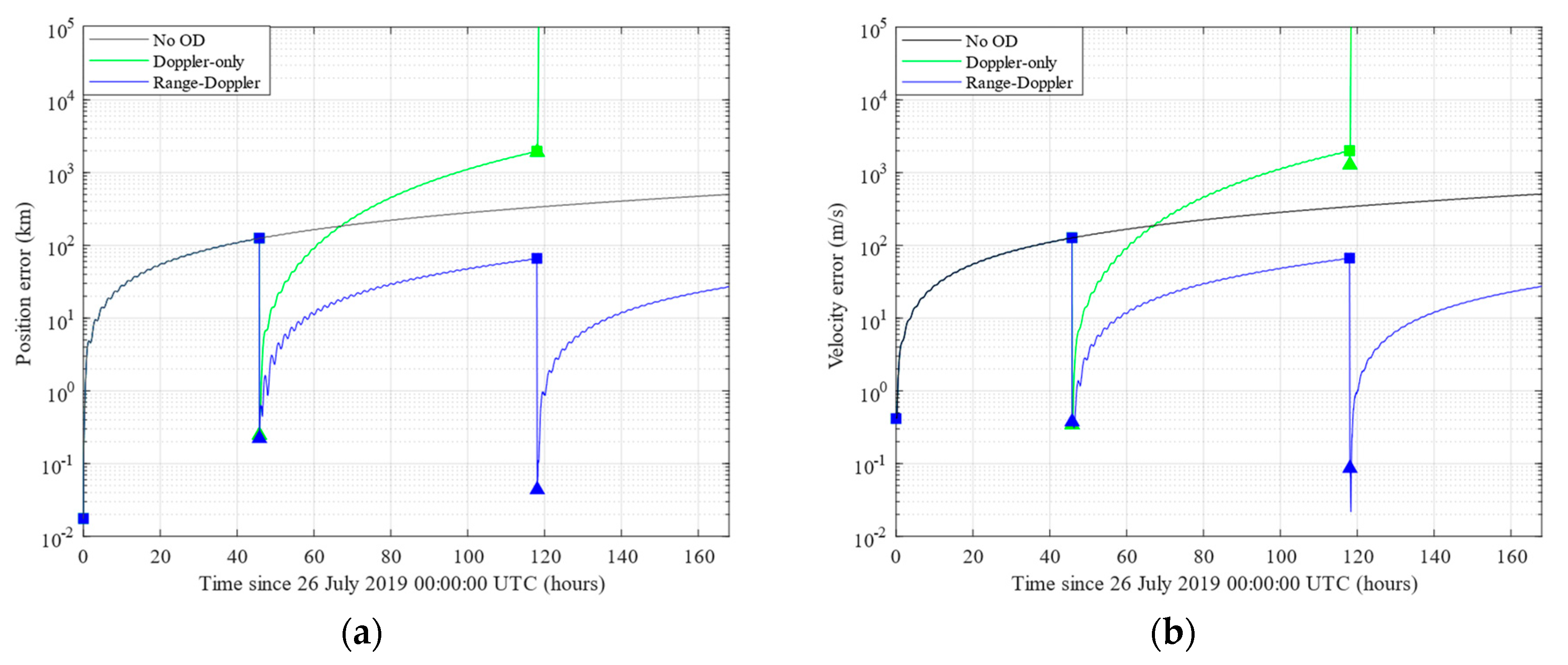
A accuracy of 10 m is assumed for the simulated slant range measurements. If slant range measurements are included, the size of the covariance matrix obtained at the end of the UKF process decreases, and this has a positive effect on the accuracy of the propagated estimate. Figure 6 shows the trend of the error in position (Figure 6a) and error in velocity (Figure 6b) obtained without OD refinement (black line), with Doppler-only UKF (green), and range-Doppler measurements (blue) for object NORAD ID 00730. Squares and triangles represent the errors at the beginning and at the end of each UKF process, respectively. As can be seen, while the accuracy of the state estimate at the end of the first UKF is similar for Doppler-only and range-Doppler OD refinement, the evolution in time is very different: the Doppler-only estimate accuracy rapidly decreases, and after the second UKF the results become unreliable. With range-Doppler measurements, instead, the error remains limited and below what can be obtained without performing OD refinement, and the average accuracy increases as the number of processed passages increases. Table 4 shows the same comparison shown in Table 3. In this case, range-Doppler measurements are considered. As can be seen, now the use of the UKF allows us to reduce the errors in position and velocity of a factor 3 and obtain an overall reduction of the size of the covariance of around one order of magnitude.
These results provide a general overview of the possible performance of BIRALET sensor for space objects tracking: Doppler shift measurements alone cannot grant accurate results for the OD refinement process, the OD improvement obtained with the UKF is rapidly lost as the error evolves in time, i.e., the growth of the error is larger than what would be obtained without OD refinement. Conversely, the combined use of Doppler shift and slant range measurements guarantees a significant improvement.
4. Conclusions
This paper introduced the novel Italian BIRALET radar system for resident space objects monitoring and tracking. A detailed description of the receiver sensor was provided in the first part of the manuscript. The receiver system consists of the Sardinia Radio Telescope, a fully steerable wheel-and-track 64-m dish located in Sardinia (Italy), with its P-band mono-beam receiver. Compared to the early years when the telescope was used for space debris measurement campaign, the system has been recently upgraded with the development of a dedicated channel for space debris monitoring. In this way, the Sardinia Radio Telescope can work with high performances in a bi-static radar configuration, providing Doppler shift and SNR measurements.
The second part of the paper was dedicated to the analysis of the orbital state estimates accuracy achievable with the sensor. The importance of the availability of possible range measurements was stressed: the combined used of Doppler and range measurement would grant both an increase in the state estimate accuracy and a reduction in the estimate uncertainty. For this reason, the most important future work will certainly be the upgrade of BIRALET to a ranging radar. The approach here presented will be tested in the future during real observation campaigns. In addition, the behavior of the sensor against the re-observation of uncatalogued objects will be investigated.
Author Contributions
L.S. performed the assembly and characterization of the space debris dedicated channel of the SRT. M.L. carried out the numerical simulations for assessing the performance of the new space debris channel. All authors prepared the article.
Funding
This research received no external funding.
Acknowledgments
The authors are grateful to the Italian Space Agency and to the National Institute for Astrophysics for the support to their research activity, and to Pierluigi Di Lizia, for his precious suggestions.
Conflicts of Interest
The authors declare no conflict of interest.
References
- Muntoni, G.; Schirru, L.; Pisanu, T.; Montisci, G.; Valente, G.; Gaudiomonte, F.; Serra, G.; Urru, E.; Ortu, P.; Fanti, A. Space Debris Detection in Low Earth Orbit with the Sardinia Radio Telescope. Electronics 2017, 6, 59. [Google Scholar] [CrossRef]
- Klinkrad, H. The Current Space Debris Environment and its Sources. In Space Debris—Models and Risk Analysis; Springer: Berlin/Heidelberg, Germany, 2006; pp. 5–58. [Google Scholar]
- Weeden, B.; Cefola, P.; Sankaran, J. Global Space Situational Awareness Sensors. In Proceedings of the Advanced Maui Optical and Space Surveillance (AMOS) Conference, Maui, HI, USA, 14–17 September 2010. [Google Scholar]
- Vallado, D.A.; Griesbach, J.D. Simulating Space Surveillance Networks. In Proceedings of the AAS/AIAA Astrodynamics Specialist Conference, Girdwood, AK, USA, 31 July–4 August 2011. [Google Scholar]
- Masekell, P.; Lorne, O. Sapphire: Canada’s Answer to Space-Based Surveillance of Orbital Objects. In Proceedings of the Advanced Maui Optical and Space Surveillance (AMOS) Conference, Maui, HI, USA, 16–19 September 2008. [Google Scholar]
- Piergentili, F.; Ceruti, A.; Rizzitelli, F.; Cardona, T.; Battagliere, M.L.; Santoni, F. Space Debris Measurement Using Joint Mid-Latitude and Equatorial Optical Observations. IEEE Trans. Aerosp. Electron. Syst. 2014, 50, 1. [Google Scholar] [CrossRef]
- Ender, J.; Leushacke, L.; Brenner, L.; Wilden, H. Radar Techniques for Space Situational Awareness. In Proceedings of the IEEE International Radar Symposium (IRS), Leipzig, Germany, 7–9 September 2011. [Google Scholar]
- Markkanen, J.; Lehtinen, M.; Landgraf, M. Real-time space debris monitoring with EISCAT. Adv Space Res. 2005, 35, 1197–1209. [Google Scholar] [CrossRef]
- Mehrholz, D.; Leushacke, L.; Jehn, R. The COBEAM-1/96 Experiment. Adv. Space Res. 1999, 23, 23–32. [Google Scholar] [CrossRef]
- Wilden, H.; Kirchner, C.; Peters, O.; Ben Bekhti, N.; Brenner, A.; Eversberg, T. GESTRA—A Phased-Array Based Surveillance and Tracking Radar for Space Situational Awareness. In Proceedings of the IEEE International Symposium on Phased Array Systems and Technology (PAST), Waltham, MA, USA, 18–21 October 2016. [Google Scholar]
- Losacco, M.; Di Lizia, P.; Massari, M.; Mattana, A.; Perini, F.; Schiaffino, M.; Bortolotti, C.; Roma, M.; Naldi, G.; Pupillo, G.; et al. The multibeam radar sensor BIRALES: Performance assessment for space surveillance and tracking. In Proceedings of the 69th International Astronautical Congress (IAC), Bremen, Germany, 1–5 October 2018. [Google Scholar]
- Pisanu, T.; Schirru, L.; Urru, E.; Gaudiomonte, F.; Ortu, P.; Bianchi, G.; Bortolotti, C.; Roma, M.; Muntoni, G.; Montisci, G.; et al. Upgrading the Italian BIRALES System to a Pulse Compression Radar for Space Debris Range Measurements. In Proceedings of the 22nd International Microwave and Radar Conference (MIKON), Poznan, Poland, 14–17 May 2018. [Google Scholar]
- Muntoni, G.; Schirru, L.; Montisci, G.; Pisanu, T.; Valente, G.; Ortu, P.; Concu, R.; Melis, A.; Saba, A.; Gaudiomonte, F.; et al. A Space Debris Dedicated Channel for the P-Band Receiver of the Sardinia Radio Telescope. IEEE Antennas Propag. Mag. in press.
- Schirru, L.; Muntoni, G.; Pisanu, T.; Urru, E.; Valente, G.; Gaudiomonte, F.; Ortu, P.; Melis, A.; Concu, R.; Bianchi, G.; et al. Upgrading the Sardinia Radio Telescope to a Bistatic Tracking Radar for Space Debris. In Proceedings of the 1st IAA Conference on Space Situational Awareness (ICSSA), Orlando, FL, USA, 13–15 November 2017. [Google Scholar]
- Tapley, B.D.; Schutz, B.E.; Born, G.H. Statistical Orbit Determination; Elsevier Academic Press: San Diego, CA, USA, 2004. [Google Scholar]
- Vallado, D.A.; Hujsak, R.S.; Johnson, T.M.; Seago, J.H.; Woodburn, J.W. Orbit Determination using ODTK version 6. Available online: https://www.researchgate.net/publication/277238110_Orbit_Determination_Using_ODTK_Version_6 (accessed on 23 September 2019).
- ExoAnalytic solutions. Available online: https://exoanalytic.com/space-situational-awareness/ (accessed on 23 September 2019).
- Bolli, P.; Orlati, A.; Stringhetti, L.; Orfei, A.; Righini, S.; Ambrosini, R.; Bartolini, M.; Bortolotti, C.; Buffa, F.; Buttu, M.; et al. Sardinia Radio Telescope: General Description, Technical Commissioning, and First Light. J. Astron. Instrum. 2015, 4, 1–20. [Google Scholar] [CrossRef]
- Bolli, P.; Olmi, L.; Roda, J.; Zacchiroli, G. A Novel Application of the Active Surface of the Shaped Sardinia Radio Telescope for Primary-Focus Operations. IEEE Antennas Wirel. Propag. Lett. 2014, 13, 1713–1716. [Google Scholar] [CrossRef]
- Schirru, L.; Pisanu, T.; Navarrini, A.; Urru, E.; Gaudiomonte, F.; Ortu, P.; Montisci, G. Advantages of Using a C-band Phased Array Feed as a Receiver in the Sardinia Radio Telescope for Space Debris Monitoring. In Proceedings of the IEEE 2nd Ukraine Conference on Electrical and Computer Engineering (UKRCON), Lviv, Ukraine, 2–6 July 2019. [Google Scholar]
- Valente, G.; Pisanu, T.; Bolli, P.; Mariotti, S.; Marongiu, P.; Navarrini, A.; Nesti, R.; Orfei, A.; Roda, J. The Dual Band L-P Feed System for the Sardinia Radio Telescope prime focus. In Millimeter, Submillimeter, and Far-Infrared Detectors and Instrumentation for Astronomy V, Proceedings of SPIE Astronomical Telescopes + Instrumentation, San Diego, CA, USA, 15 July 2010; International Society for Optics and Photonics: San Diego, CA, USA, 2010; p. 774126. [Google Scholar]
- Nicolini, L.; Caporali, A. Investigation of Reference Frames and Tim Systems in Multi-GNSS. Remote Sens. 2018, 10, 80. [Google Scholar]
- Wan, E.; Van Der Merwe, R. Chapter 7: The Unscented Kalman Filter. In Kalman Filtering and Neural Networks; Wiley: New York, NY, USA, 2001; pp. 221–280. [Google Scholar]
Figure 1.
Picture of the Sardinia Radio Telescope (SRT) in a typical measurement campaign.

Figure 2.
Picture of the L-P cryogenic receiver (red circled) installed on the SRT primary focus.

Figure 3.
Scheme of the dedicated space debris signal acquisition chain of the SRT.

Figure 4.
Simplified measurement setup, used in the first space debris experiment with the SRT.
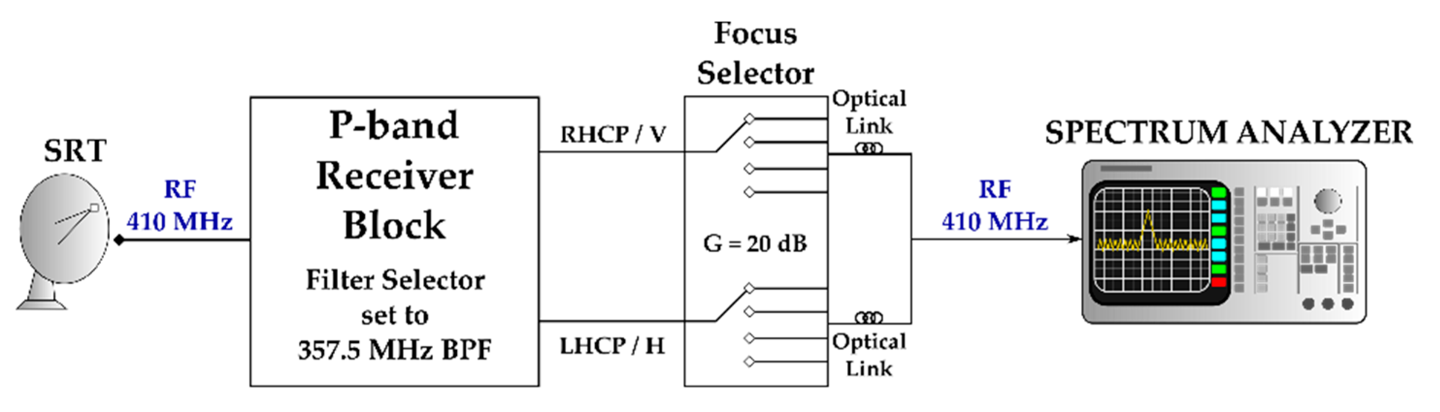
Figure 5.
SRT observation capabilities: (a) orbital inclination as a function of the perigee height, (b) number of passages per object.
Figure 5.
SRT observation capabilities: (a) orbital inclination as a function of the perigee height, (b) number of passages per object.
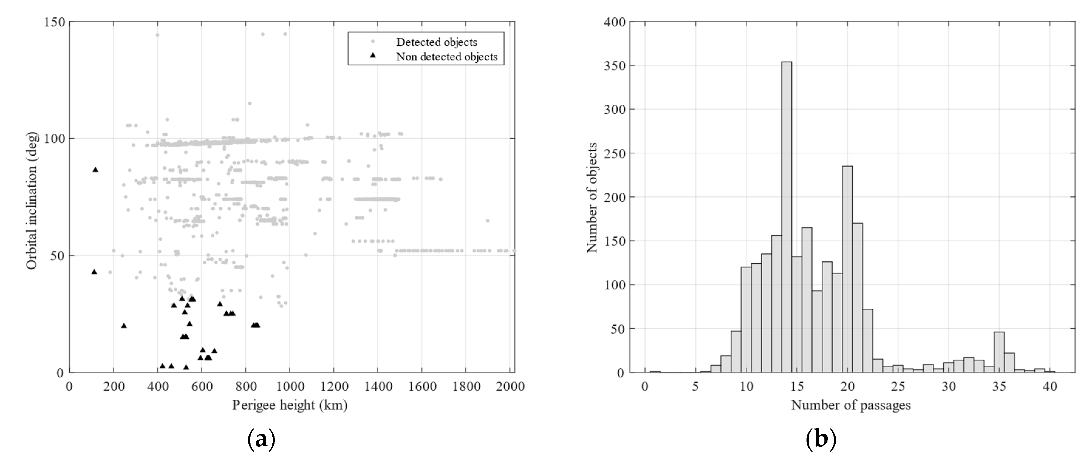
Figure 6.
Object NORAD ID 00730, error in position (a) and velocity (b) as a function of time without performing OD refinement (black line), with Doppler-only (green) and range-Doppler (blue) OD refinement. Squares and triangles represent the error before and after the UKF, respectively.
Figure 6.
Object NORAD ID 00730, error in position (a) and velocity (b) as a function of time without performing OD refinement (black line), with Doppler-only (green) and range-Doppler (blue) OD refinement. Squares and triangles represent the error before and after the UKF, respectively.

Table 1.
Main characteristics of the SRT, focusing on P-band (410 MHz).
| Optics | Gregorian (Shaped) + BWG |
|---|---|
| Focal Positions | Primary: f/D = 0.33 |
| Gregorian: f/D = 2.34 | |
| 2 x BWG I: f/D = 1.38 | |
| 2 x BWG II: f/D = 2.81 | |
| Frequency Range | 0.3 − 116 GHz |
| Primary Reflector Diameter | 64 m |
| Secondary Reflector Diameter | 7.9 m |
| BWG Mirrors Diameter | 2.9 − 3.9 m |
| Azimuth and Elevation Speed (wind speed < 60 km/h) | 0.85 °/s (Az) |
| 0.5 °/s (El) | |
| Azimuth and Elevation Range pointing | 5 ÷ 90° (Az) |
| −270° ÷ +270° (El) | |
| Antenna Gain at 410 MHz | 46.6 dBi |
| Antenna Efficiency at 410 MHz | 57.7% |
| Half Power Beam Width (HPBW) at 410 MHz | 0.8° |
| System noise temperature | about 25 K |
| System noise power | about −100 dBm |
| Typical received SNR level | >10 dB |
Table 2.
Doppler-only performance for object NORAD ID 00730 at different time epochs, in terms of error in position and velocity ( and ) and standard deviation in position and velocity ( and ) obtained performing OD refinement (“OD” subscript) or without updating the estimate (“free” subscript).
Table 2.
Doppler-only performance for object NORAD ID 00730 at different time epochs, in terms of error in position and velocity ( and ) and standard deviation in position and velocity ( and ) obtained performing OD refinement (“OD” subscript) or without updating the estimate (“free” subscript).
| Epoch (UTC) | ||||||||
|---|---|---|---|---|---|---|---|---|
| 26/07/2019 00:00:00 | - | - | - | - | 1.76e-2 | 2.45e-1 | 4.16e-1 | 1.73 |
| 27/07/2019 21:46:25 | - | - | - | - | 1.26e2 | 5.01e2 | 1.27e2 | 5.08e2 |
| 27/07/2019 21:48:09 | 2.46e-1 | 2.86 | 3.41e-1 | 4.17 | 1.26e2 | 5.01e3 | 1.27e2 | 5.08e2 |
| 28/07/2019 21:48:09 | 2.35e2 | 1.80e3 | 2.39e2 | 1.83e3 | 1.93e2 | 7.63e2 | 1.96e2 | 7.74e2 |
| 29/07/2019 21:48:09 | 8.82e2 | 3.76e3 | 9.01e2 | 3.82e3 | 2.62e2 | 1.03e3 | 2.66e2 | 1.04e3 |
Table 3.
Doppler-only orbit determination (OD) performance in terms of median (50% superscript) of the error in position and velocity ( and ) and standard deviation in position and velocity ( and ) obtained with (“OD” subscript) and without (“free“ subscript) OD refinement, and median of the and indexes. All quantities are referred to epoch 02 August 2019 00:00:00 UTC.
| 1.76e3 | 3.19e3 | 1.74 | 3.11 | 4.80e2 | 1.85e3 | 4.47e-1 | 1.83 | 1.72 | 1.74 |
Table 4.
Range-Doppler OD performance in terms of median (50% superscript) of the error in position and velocity ( and ) and standard deviation in position and velocity ( and ) obtained with (“OD” subscript) and without (“free” subscript) OD refinement, and median of the and indexes. All quantities are referred to epoch 02 August 2019 00:00:00 UTC.
| 1.19e2 | 1.98e2 | 1.15e-1 | 1.91e-1 | 4.81e2 | 1.85e3 | 4.47e-1 | 1.83 | 1.09e-1 | 1.09e-1 |
© 2019 by the authors. Licensee MDPI, Basel, Switzerland. This article is an open access article distributed under the terms and conditions of the Creative Commons Attribution (CC BY) license (http://creativecommons.org/licenses/by/4.0/).
Share and Cite
MDPI and ACS Style
Losacco, M.; Schirru, L. Orbit Determination of Resident Space Objects Using the P-Band Mono-Beam Receiver of the Sardinia Radio Telescope. Appl. Sci. 2019, 9, 4092. https://doi.org/10.3390/app9194092
AMA Style
Losacco M, Schirru L. Orbit Determination of Resident Space Objects Using the P-Band Mono-Beam Receiver of the Sardinia Radio Telescope. Applied Sciences. 2019; 9(19):4092. https://doi.org/10.3390/app9194092
Chicago/Turabian StyleLosacco, Matteo, and Luca Schirru. 2019. "Orbit Determination of Resident Space Objects Using the P-Band Mono-Beam Receiver of the Sardinia Radio Telescope" Applied Sciences 9, no. 19: 4092. https://doi.org/10.3390/app9194092
Note that from the first issue of 2016, this journal uses article numbers instead of page numbers. See further details here.