Optimal Operation of Isolated Microgrids Considering Frequency Constraints

 , ,
, ,
Abstract
:1. Introduction
1.1. Literature Review
1.2. Required Improvements in the EMS Development for Isolated Microgrids
1.3. Paper Contributions
- The parameters that, being available by the EMS, may influence the frequency deviations are analyzed.
- The the maximum frequency deviation in front of the maximum power imbalance is formulated. This formulation uses the above-mentioned parameters.
- An EMS including a frequency constraint is formulated.
- The validation of the proposed EMS using dynamic simulation and laboratory platform is presented.
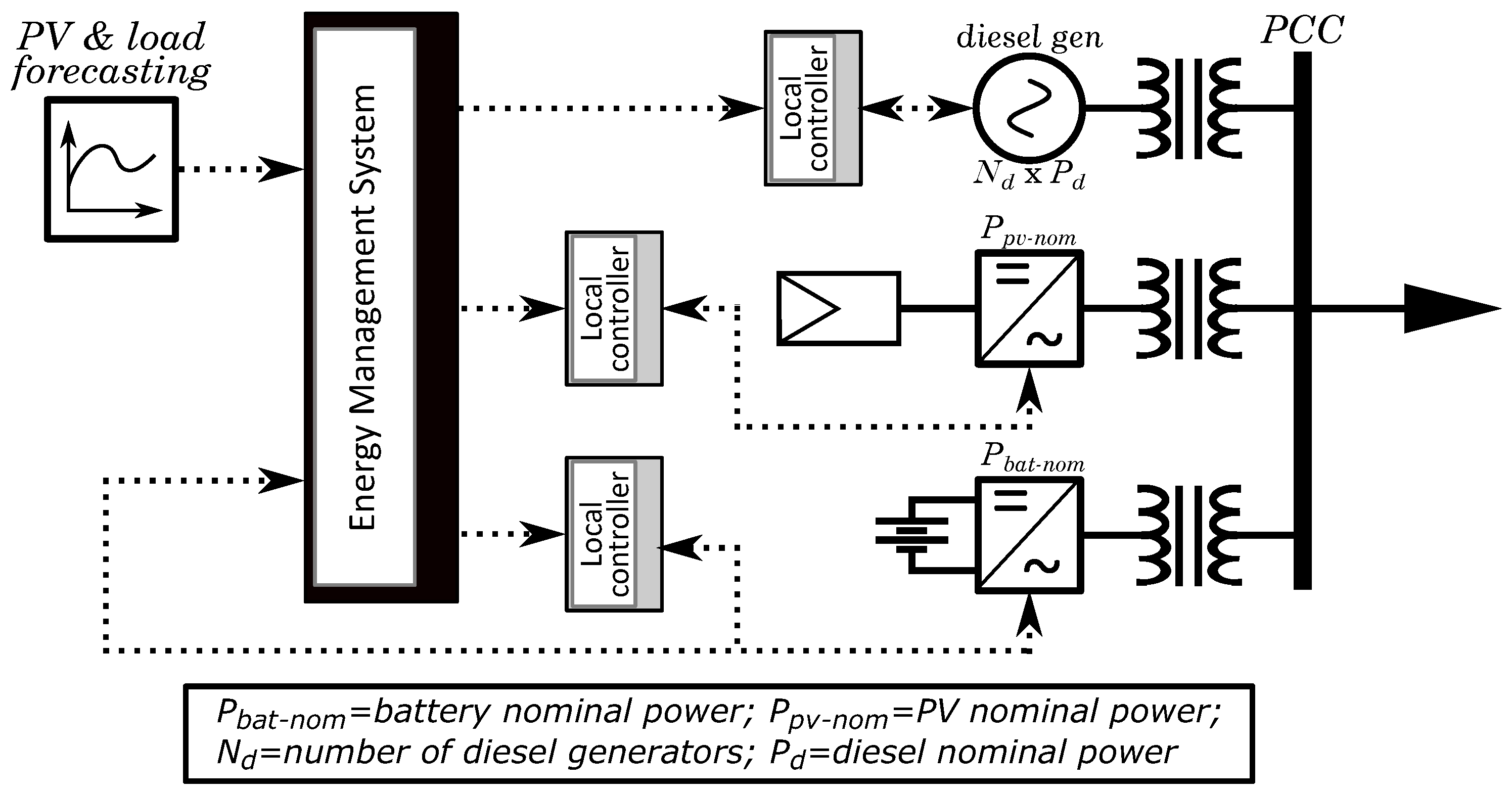
2. System Description
- LC for diesel generation power plant: The local controller is in charge of controlling the frequency of the grid. A proportional–integral (PI) controller, where the input is the frequency error (filtered by a low pass filter), computes the mechanical torque setpoint of each diesel generator. This local controller also receives the required number of connected diesel generators and accordingly sends orders of connection/disconnection to each diesel unit. Each diesel generator has its internal controller in charge of reaching the torque setpoint and to perform its connection and disconnection according to the LC requirements. A similar control architecture is found in [23]. The main difference is that in the present paper the PI is a central controller that coordinates all the diesel units, while in [23] a single unit is considered.
- LC for the PV power plant: This LC implements a power–frequency droop curve to provide support to the grid. Reducing the active power will always be possible, but increasing it (under frequency events) will depend on the available active power. The controller can perform power curtailments. A maximum PV power setpoint is received externally and a PI controller computes the active power setpoint of each PV inverter. This controller is defined in [24], but the ramp rate limitation is not taken into account.
- LC for the battery: This controller receives externally an active power sepoint and applies a power–frequency droop curve to provide grid support. The output is the droop modified setpoint. The inner control loops will be in charge of reaching this value of active power. The dynamic model is simplified as in [25], but the local frequency droop has been included.
3. Methodology
3.1. EMS Design Requirements
3.2. EMS Performance
3.3. Execution Cycle
3.4. Modeling Frequency Deviations
3.5. Scenarios Generation
3.6. Stochastic Formulation Approach
3.7. Formulation of the Optimization Algorithm
3.7.1. Sets
3.7.2. Decision Variables
3.7.3. Parameters
3.7.4. Objective Function
3.7.5. Constraints
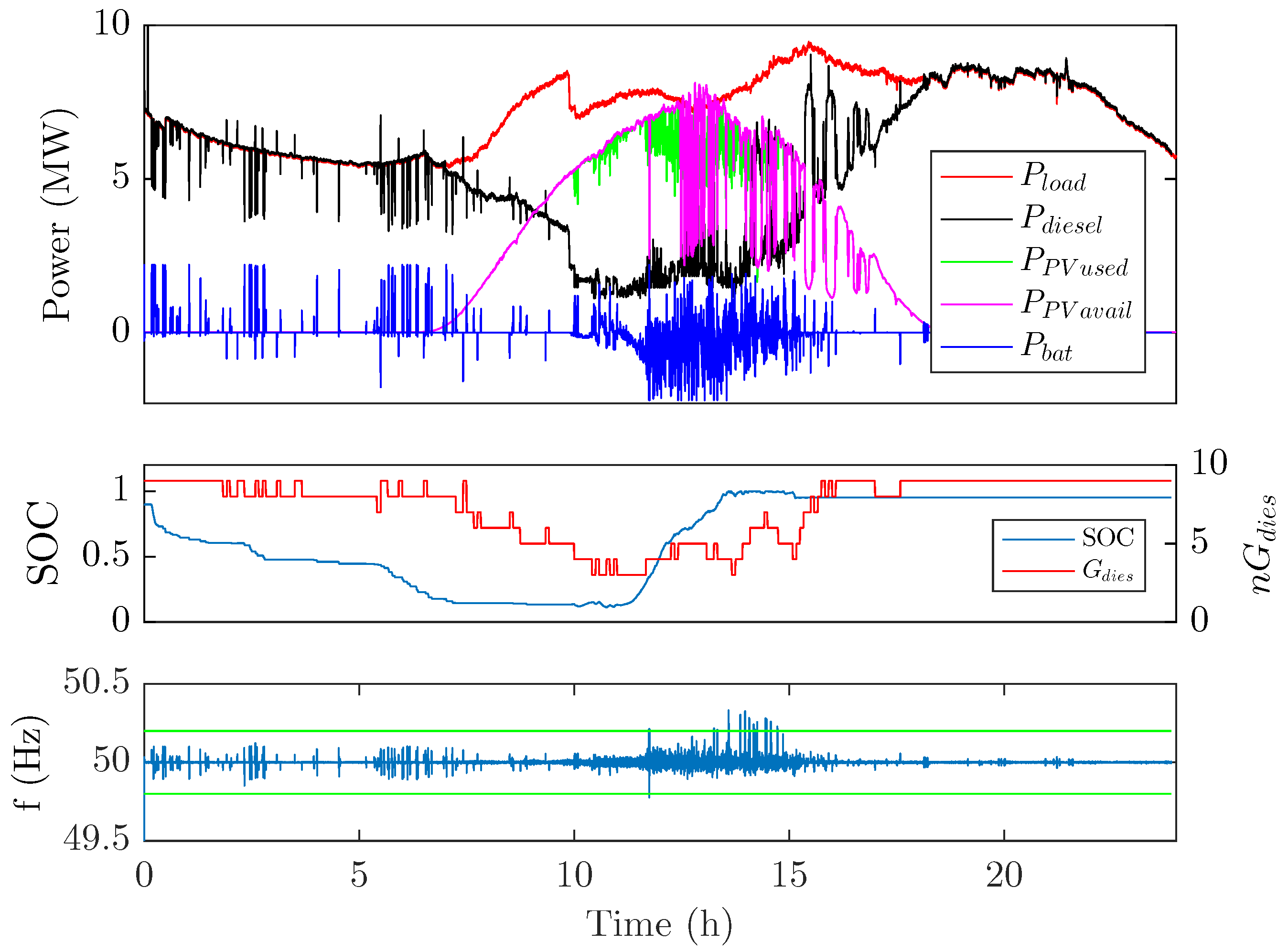
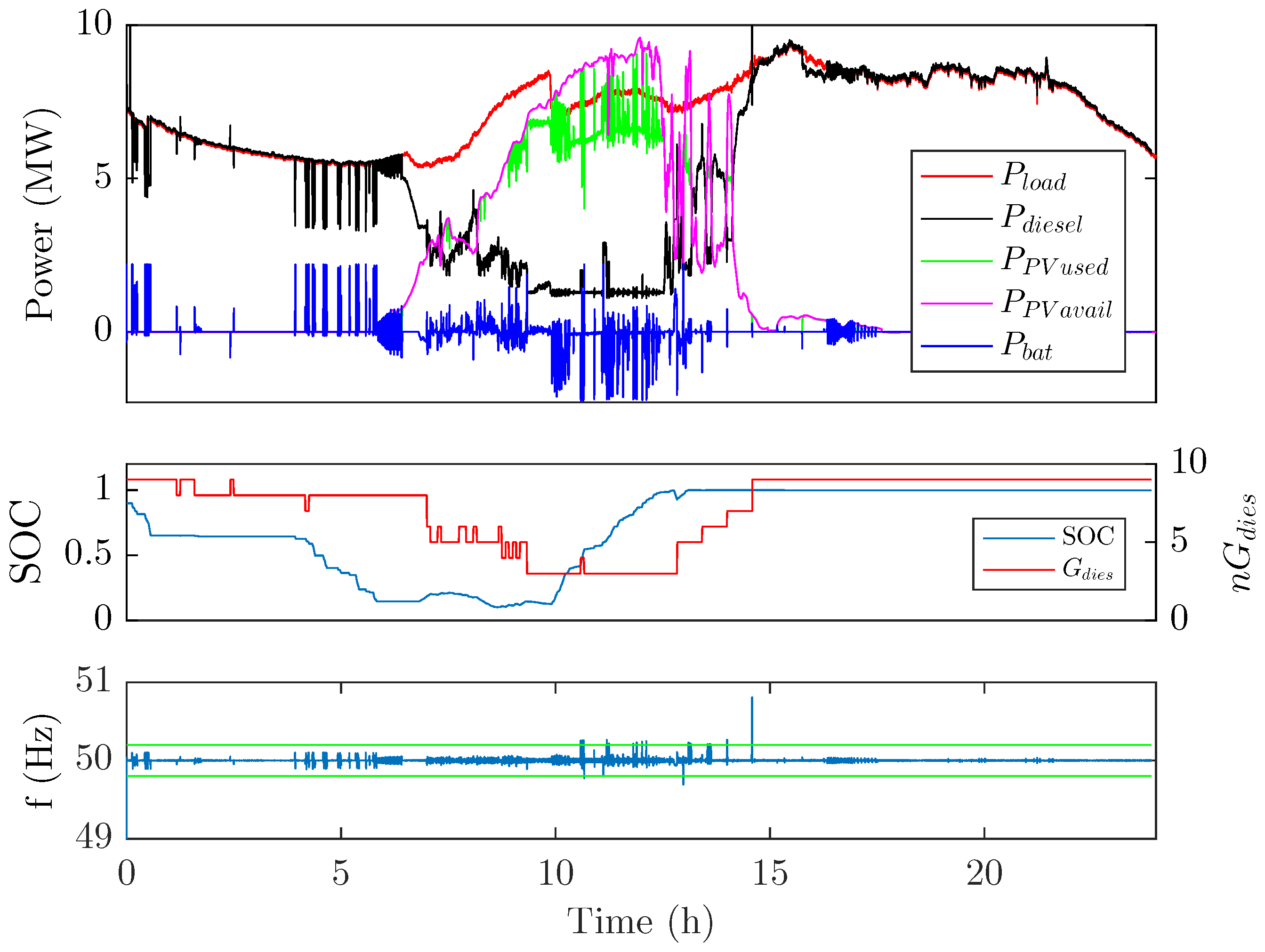
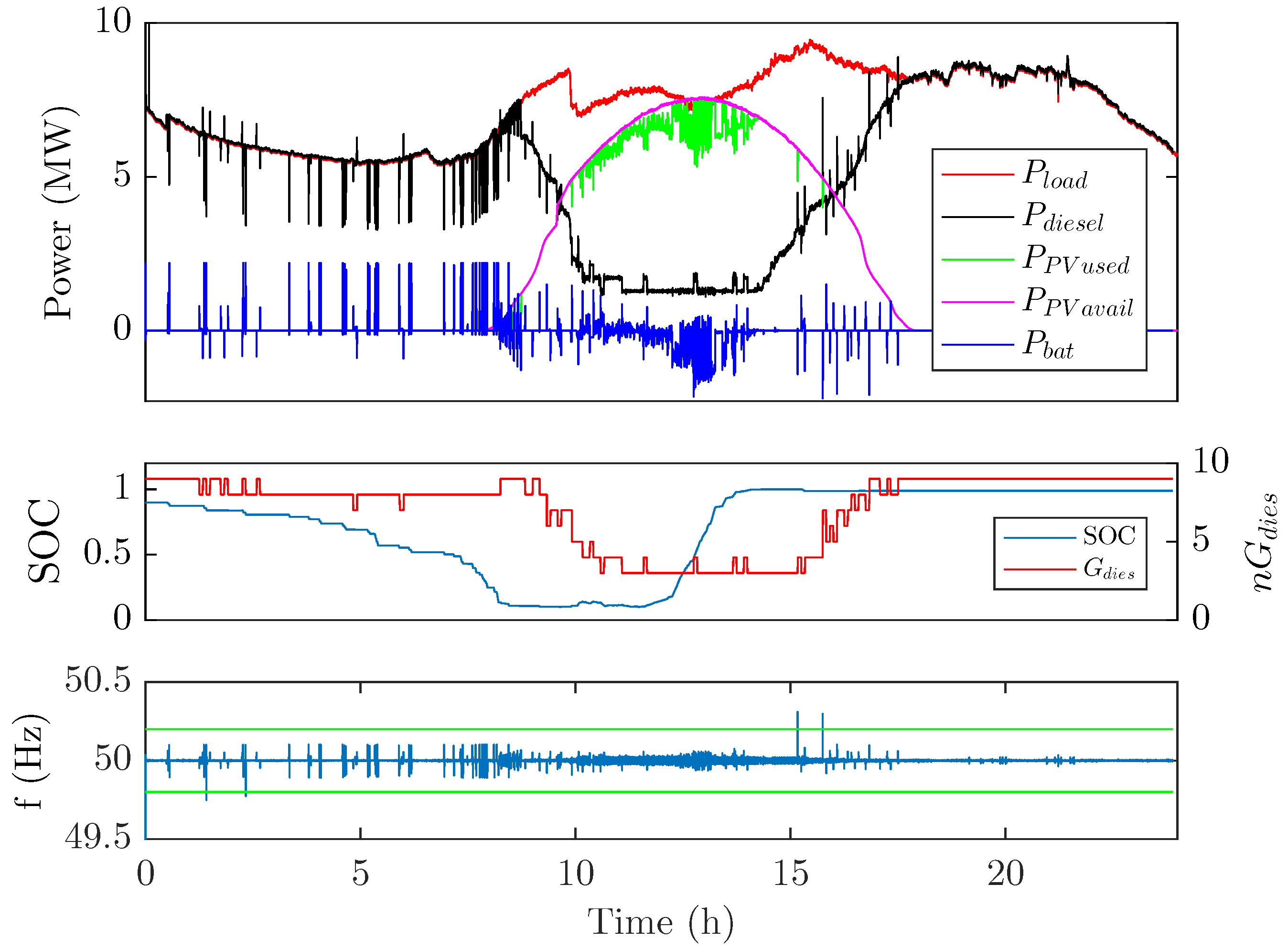
4. Case Study
5. Experimental Validation
5.1. Platform Description
5.2. Emulation Results
6. Conclusions
Author Contributions
Funding
Acknowledgments
Conflicts of Interest
References
- Aegerl, C.S.; Tao, L. The Microgrids Concept. In Microgrids Architectures and Control; Hatziargyriou, N., Ed.; John Wiley and Sons: Hoboken, NJ, USA, 2013. [Google Scholar]
- DOE. Summary Report: 2012 DOE Microgrid Workshop; DOE: Washington, DC, USA, 2012.
- Bullich-Massagué, E.; Díaz-González, F.; Aragüés-Peñalba, M.; Girbau-Llistuella, F.; Olivella-Rosell, P.; Sumper, A. Microgrid clustering architectures. Appl. Energy 2018, 212, 340–361. [Google Scholar] [CrossRef]
- Neely, J.; Johnson, J.; Delhotal, J.; Gonzalez, S.; Lave, M. Evaluation of PV frequency-watt function for fast frequency reserves. In Proceedings of the 2016 IEEE Applied Power Electronics Conference and Exposition (APEC), Long Beach, CA, USA, 20–24 March 2016; pp. 1926–1933. [Google Scholar] [CrossRef]
- Kundur, P.; Balu, N.; Lauby, M. Power System Stability and Control; EPRI Power System Engineering Series; McGraw-Hill: New York, NY, USA, 1994. [Google Scholar]
- Martin-Martínez, F.; Sánchez-Miralles, A.; Rivier, M. A literature review of Microgrids: A functional layer based classification. Renew. Sustain. Energy Rev. 2016, 62, 1133–1153. [Google Scholar] [CrossRef]
- Han, Y.; Shen, P.; Zhao, X.; Guerrero, J.M. Control Strategies for Islanded Microgrid Using Enhanced Hierarchical Control Structure With Multiple Current-Loop Damping Schemes. IEEE Trans. Smart Grid 2017, 8, 1139–1153. [Google Scholar] [CrossRef]
- Vandoorn, T.L.; Vasquez, J.C.; Kooning, J.D.; Guerrero, J.M.; Vandevelde, L. Microgrids: Hierarchical Control and an Overview of the Control and Reserve Management Strategies. IEEE Ind. Electron. Mag. 2013, 7, 42–55. [Google Scholar] [CrossRef] [Green Version]
- Bidram, A.; Davoudi, A. Hierarchical Structure of Microgrids Control System. IEEE Trans. Smart Grid 2012, 3, 1963–1976. [Google Scholar] [CrossRef]
- Parisio, A.; Rikos, E.; Glielmo, L. A Model Predictive Control Approach to Microgrid Operation Optimization. IEEE Trans. Control Syst. Technol. 2014, 22, 1813–1827. [Google Scholar] [CrossRef]
- Marzband, M.; Sumper, A.; Domínguez-García, J.L.; Gumara-Ferret, R. Experimental validation of a real time energy management system for microgrids in islanded mode using a local day ahead electricity market and MINLP. Energy Convers. Manag. 2013, 76, 314–322. [Google Scholar] [CrossRef]
- Marzband, M.; Yousefnejad, E.; Sumper, A.; Domínguez-García, J.L. Real time experimental implementation of optimum energy management system in standalone Microgrid by using multi layer ant colony optimization. Int. J. Electr. Power Energy Syst. 2016, 75, 265–274. [Google Scholar] [CrossRef]
- Marzband, M.; Ghadimi, M.; Sumper, A.; Domínguez-García, J.L. Experimental validation of a real-time energy management system using multi period gravitational search algorithm for microgrids in islanded mode. Appl. Energy 2014, 128, 164–174. [Google Scholar] [CrossRef]
- Chen, C.; Duan, S.; Cai, T.; Liu, B.; Hu, G. Smart energy management system for optimal microgrid economic operation. IET Renew. Power Gener. 2011, 5, 258–267. [Google Scholar] [CrossRef]
- Sobu, A.; Wu, G. Optimal operation planning method for isolated micro grid considering uncertainties of renewable power generations and load demand. In Proceedings of the IEEE PES Innovative Smart Grid Technologies, Tianjin, China, 21–24 May 2012; pp. 1–6. [Google Scholar] [CrossRef]
- Lazaroiu, G.C.; Dumbrava, V.; Balaban, G.; Longo, M.; Zaninelli, D. Stochastic optimization of microgrids with renewable and storage energy systems. In Proceedings of the 2016 IEEE 16th International Conference on Environment and Electrical Engineering (EEEIC), Florence, Italy, 7–10 June 2016; pp. 1–5. [Google Scholar] [CrossRef]
- Cau, G.; Cocco, D.; Petrollese, M.; Kær, S.K.; Milan, C. Energy management strategy based on short-term generation scheduling for a renewable microgrid using a hydrogen storage system. Energy Convers. Manag. 2014, 87, 820–831. [Google Scholar] [CrossRef]
- Palma-Behnke, R.; Benavides, C.; Lanas, F.; Severino, B.; Reyes, L.; Llanos, J.; Sáez, D. A Microgrid Energy Management System Based on the Rolling Horizon Strategy. IEEE Trans. Smart Grid 2013, 4, 996–1006. [Google Scholar] [CrossRef]
- Zhao, B.; Xue, M.; Zhang, X.; Wang, C.; Zhao, J. An {MAS} based energy management system for a stand-alone microgrid at high altitude. Appl. Energy 2015, 143, 251–261. [Google Scholar] [CrossRef]
- Sanseverino, E.R.; Nguyen, N.Q.; Silvestre, M.L.D.; Zizzo, G.; de Bosio, F.; Tran, Q.T.T. Frequency constrained optimal power flow based on glow-worm swarm optimization in islanded microgrids. In Proceedings of the 2015 AEIT International Annual Conference (AEIT), Naples, Italy, 14–16 October 2015; pp. 1–6. [Google Scholar] [CrossRef]
- Zhang, G.; McCalley, J. Optimal power flow with primary and secondary frequency constraint. In Proceedings of the 2014 North American Power Symposium (NAPS), Pullman, WA, USA, 7–9 September 2014; pp. 1–6. [Google Scholar] [CrossRef]
- Díaz-González, F.; Hau, M.; Sumper, A.; Gomis-Bellmunt, O. Participation of wind power plants in system frequency control: Review of grid code requirements and control methods. Renew. Sustain. Energy Rev. 2014, 34, 551–564. [Google Scholar] [CrossRef]
- Theubou, T.; Wamkeue, R.; Kamwa, I. Dynamic model of diesel generator set for hybrid wind-diesel small grids applications. In Proceedings of the 2012 25th IEEE Canadian Conference on Electrical and Computer Engineering (CCECE), Montreal, QC, Canada, 29 April–2 May 2012; pp. 1–4. [Google Scholar] [CrossRef]
- Bullich-Massagué, E.; Ferrer-San-José, R.; Aragüés-Peñalba, M.; Serrano-Salamanca, L.; Pacheco-Navas, C.; Gomis-Bellmunt, O. Power plant control in large-scale photovoltaic plants: Design, implementation and validation in a 9.4 MW photovoltaic plant. IET Renew. Power Gener. 2016, 10, 50–62. [Google Scholar] [CrossRef]
- Bullich-Massagué, E.; Aragüés-Peñalba, M.; Sumper, A.; Boix-Aragones, O. Active power control in a hybrid PV-storage power plant for frequency support. Sol. Energy 2017, 144, 49–62. [Google Scholar] [CrossRef]
- Prieto-Araujo, E.; Olivella-Rosell, P.; Cheah-Mañe, M.; Villafafila-Robles, R.; Gomis-Bellmunt, O. Renewable energy emulation concepts for microgrids. Renew. Sustain. Energy Rev. 2015, 50, 325–345. [Google Scholar] [CrossRef] [Green Version]


| Parameter | Value | Parameter | Value | Parameter | Value |
|---|---|---|---|---|---|
| 288 | 1120 kWh | −2200 kW | |||
| 10 | 0.9 | 0.3·1100 kW | |||
| 9 | 0.9 | 1100 kW | |||
| 5 | 2200 kW | 2000 kW |
© 2019 by the authors. Licensee MDPI, Basel, Switzerland. This article is an open access article distributed under the terms and conditions of the Creative Commons Attribution (CC BY) license (http://creativecommons.org/licenses/by/4.0/).
Share and Cite
Vidal-Clos, J.-A.; Bullich-Massagué, E.; Aragüés-Peñalba, M.; Vinyals-Canal, G.; Chillón-Antón, C.; Prieto-Araujo, E.; Gomis-Bellmunt, O.; Galceran-Arellano, S. Optimal Operation of Isolated Microgrids Considering Frequency Constraints. Appl. Sci. 2019, 9, 223. https://doi.org/10.3390/app9020223
Vidal-Clos J-A, Bullich-Massagué E, Aragüés-Peñalba M, Vinyals-Canal G, Chillón-Antón C, Prieto-Araujo E, Gomis-Bellmunt O, Galceran-Arellano S. Optimal Operation of Isolated Microgrids Considering Frequency Constraints. Applied Sciences. 2019; 9(2):223. https://doi.org/10.3390/app9020223
Chicago/Turabian StyleVidal-Clos, Josep-Andreu, Eduard Bullich-Massagué, Mònica Aragüés-Peñalba, Guillem Vinyals-Canal, Cristian Chillón-Antón, Eduardo Prieto-Araujo, Oriol Gomis-Bellmunt, and Samuel Galceran-Arellano. 2019. "Optimal Operation of Isolated Microgrids Considering Frequency Constraints" Applied Sciences 9, no. 2: 223. https://doi.org/10.3390/app9020223