Iterative Phase-Only Hologram Generation Based on the Perceived Image Quality


1
Joint International Research Laboratory of Information Display and Visualization, School of Electronic Science and Engineering, Southeast University, Nanjing 210096, China
2
Centre for Photonic Devices and Sensors, Department of Engineering, University of Cambridge, 9 JJ Thomson Avenue, Cambridge CB3 0FA, UK
*
Authors to whom correspondence should be addressed.
Appl. Sci. 2019, 9(20), 4457; https://doi.org/10.3390/app9204457
Submission received: 5 October 2019
/
Revised: 13 October 2019
/
Accepted: 17 October 2019
/
Published: 21 October 2019
(This article belongs to the Special Issue Practical Computer-Generated Hologram for 3D Display)
Abstract
:Image quality metrics are a critical element in the iterative Fourier transform algorithms (IFTAs) for the computer generation of phase-only holograms. Conventional image quality metrics such as root-mean-squared error (RMSE) are sensitive to image content and unable to reflect the perceived image quality accurately. This would have a significant impact on the calculation speed and the quality of the generated hologram. In this work, the structure similarity (SSIM) was proposed as an image quality metric in IFTAs due to its ability to predict the perceived image quality in the presence of the white Gaussian noise and its independence on the image content. This would enable IFTAs to terminate when further iterations would no longer lead to improvement in the perceived image quality. As a result, up to 75% of unnecessary iterations were eliminated by the use of SSIM as the image quality metric.
1. Introduction
Phase-only holograms can be used for 2-D [1,2,3,4] or 3-D image projection [5,6], free space optical switches [7,8,9,10,11] and optical tweezers [12,13]. These systems generally enjoy a high efficiency due to the absence of any light absorbing element such as cross-polarizers [14]. Two-dimensional image projection is one of the most mature applications due to the simplicity of the optical systems and its high tolerance to system errors [4]. In order to form the target image, however, the phase-only hologram needs to be calculated in the first place. This is usually a computationally intensive process. Iterative Fourier transform algorithms (IFTAs) [15] including Gerchberg–Saxton (GS) [16], Fienup [17], and ‘Fienup with don’t-care’ (FiDOC) [18,19], are able to accelerate the calculation significantly by using the fast Fourier transform (FFT). In these algorithms, the errors in the image reconstructed from the computer-generated phase-only hologram are evaluated based on certain key image quality metrics at the end of each iteration. The iteration process is terminated until a predefined requirement is satisfied or the number of the iteration reaches the predefined threshold. Therefore, the image quality metrics used in IFTA algorithms should be able to reflect the perceived image quality [20] in the phase-only holographic projection system. It will directly affect both the quality of the reconstructed image and the speed of the algorithm.
The choice of the image quality metrics is dependent on the specific type of errors in the reconstructed images. Chu et al. [21] proposed some effective statistical methods to characterize the noise of a large number of samples and revealed that the noise usually has a Poisson or Gaussian distribution. These methods have the potential to be applied to investigate the noise characteristics in the images reconstructed from the phase-only holograms calculated by IFTAs. Georgiou et al. [4] investigated the probability density function (PDF) for the grey-scale values in a reconstructed chessboard pattern. However, it did not identify the type of noise in the reconstructed images. This work aims to further study the noise characteristics in the images reconstructed from the phase-only holograms that are calculated by IFTAs.
At present, the root-mean-squared error (RMSE) [22,23] is the most widely used image quality metric in IFTAs. Gerchberg et al. proved that the RMSE would always converge towards a lower value as the iteration moved forward in IFTAs. The speed of convergence is usually quicker in Fienup algorithm than in the standard GS algorithm. However, it has been proved that RMSE was unable to reflect the perceived image quality accurately [24]. In other words, reconstructed images with similar values of RMSE might have a significantly different perceived image quality.
Efforts have been made to establish the relationship between the objective image quality metrics and the subjective image quality. Just-noticeable difference (JND) [25] has been proposed to define the subjective image quality and it has been linked with the luminance and color characteristics of the display system [26,27]. Barten [28] proposed the square-root integral (SQRI) to evaluate the image quality. However, the calculation of SQRI is rather complicated. Wang et al. [24,29] proved that structure similarity (SSIM) is a simple and consistent image quality metric to assess the perceived quality of images. This work will investigate the suitability of SSIM as the image quality metric in the IFTAs. To authors’ knowledge, it is the first time that the perceived image quality is used in the IFTAs for the phase-only hologram generation.
2. Existing IFTAs
GS algorithm [16] is the most widely used algorithm for the computer generation of phase-only holograms. GS algorithm involves iterative calculation of the light field distributions on the hologram plane and the image plane via a known propagating function of the optical system. In most cases, the propagating function is the Fourier transform. One loop of GS can be mathematically described as:
where and are the light field distributions at the hologram plane and image plane, respectively; FT and FT−1 represent the Fourier transform and the inverse Fourier transform, respectively; and G0 is the intensity of the target image. The initial field distribution at the image plane, g0, is assigned G0 multiplied by a random phase. Then the loop will be repeated until the reconstructed image quality meets the requirement.
The GS algorithm is very stable and always leads to convergence. However, it usually needs a large number of iterations to achieve a reasonably good image quality. To improve the calculation speed, various derivatives of the GS algorithm have been developed, most notably among them Fienup [17] and FiDOC [18,19]. In the Fienup algorithm, Equation (5) is used to replace the standard Equation (4) in the standard GS algorithm. This introduces the feedback mechanism into the iterations.
The Gn in this equation is expressed as:
where k is the feedback coefficient.
FiDOC algorithm further improved Fienup algorithm by assigned areas around the target images as the don’t-care area. The don’t-care area on the image plane allows noise on the hologram plane in the form of spatial frequency components. As a result, the reconstruction quality in the don’t-care area is sacrificed while the image quality in the target area is enhanced. Correspondingly, the feedback function for Gn is changed into [18,19]:
where is the noise suppression parameter for the image plane; M equals 1 within and the target area and 0 in the don’t-care area.
3. Noise Characteristics in the Reconstructed Images
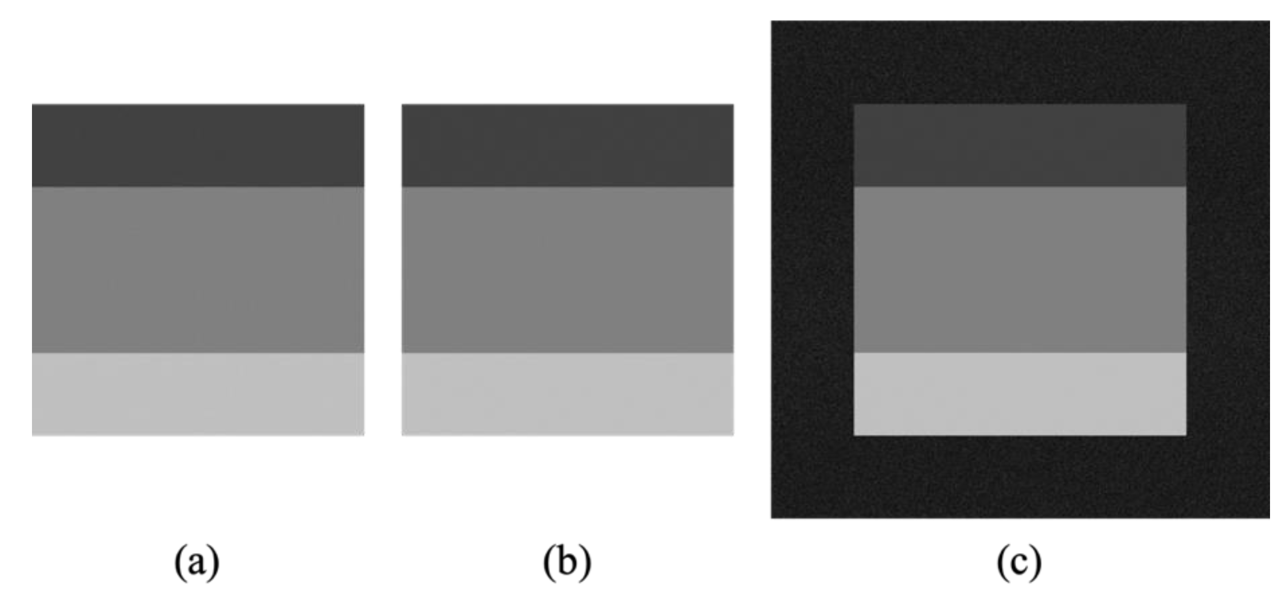
The perceived image quality could depend on the type of distortions in the image. In this work, the test image pattern shown in Figure 1 is used to investigate the noise characteristics in the reconstructed images from the holograms calculated by IFTAs. The pattern had 512 × 512 pixels and consisted of three areas from the top to the bottom. The top and the bottom areas had the exact same dimensions of 128 × 512 pixels and the corresponding grey values were 64 and 192, respectively. The middle area had 256 × 512 pixels with a grey value of 128.
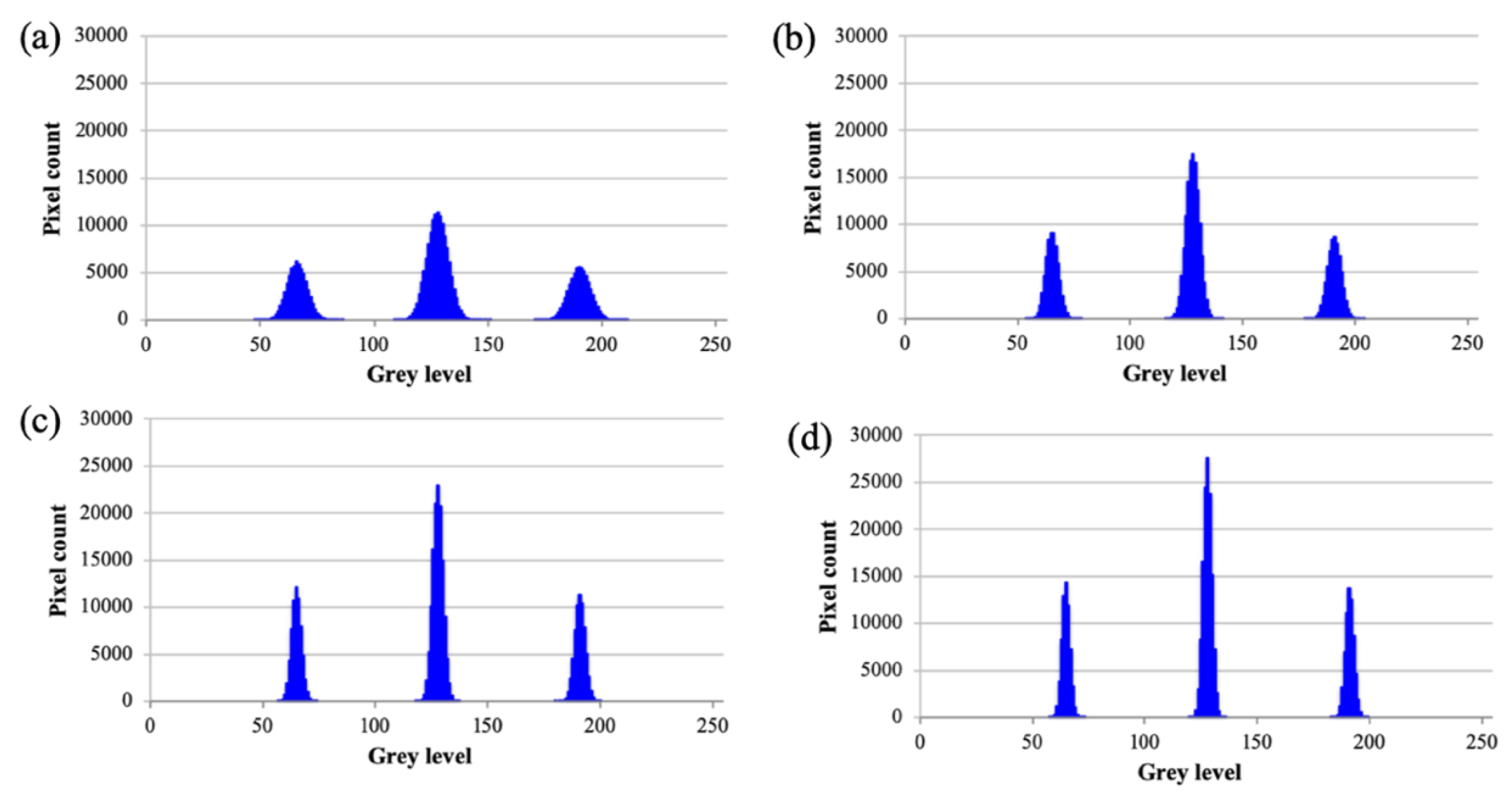
First, the standard GS algorithm was used to calculate the phase-only holograms that were able to reconstruct this target image pattern in Figure 1. Figure 2 shows the reconstructed images after 50, 100, 150 and 200 GS iterations. The differences between them are small but still can be perceived by human eyes. It can be seen that the quality of the reconstructed images is improved as the number of iterations increases. Figure 3 shows the histograms of grey values in these images. It can be seen that the distributions of the grey values are a superposition of three Gaussian distributions. Fittings for these grey value distributions were carried out based on the following equation:
The fitting results are listed in Table 1. The coefficient of determination, i.e., r2, is >0.999 for all of the fittings. This indicates that Equation (8) is able to reflect the grey value distribution in the reconstructed images accurately. Therefore, the noise in the reconstructed images has a Gaussian distribution. The improvement in the quality of the reconstructed image as the iteration progresses can be reflected by the decrease in the Gaussian variance, i.e., values of δ1, δ2 and δ3. In other words, the reconstructed images are less affected by white Gaussian noise with increased number of GS iterations.
Fienup and FiDOC algorithms were also used to calculate the phase-only holograms. In the FiDOC algorithm, the don’t-care area accounts for 25% of the original image in this dimension. Therefore, the total dimension became 640 × 640 pixels. Figure 4 compares the reconstructed images from the calculated holograms after 200 GS, Fienup and FiDOC iterations. It can be seen that both the Fienup and FiDOC algorithms outperformed the GS algorithm. The distributions of the grey values in these three reconstructed images are plotted in Figure 5.
The corresponding fitting results based on Equation (8) are listed in Table 2. It should be noted that the results for Figure 4c only include the target area. Again, the coefficient of determination, i.e., r2, exceeds 0.9999 in all these three fittings. This further confirms the main source of distortion in the images reconstructed from the holograms calculated by IFTAs is the white Gaussian noise. Different types of IFTAs will only lead to different degrees of white Gaussian noise in the reconstructed images.
4. Image Quality Metrics and Perceived Image Quality
IFTAs need to perform a number of iterations to achieve a good reconstructed image quality. The number of iterations that is required usually depends the image content. In practice, an image quality metric is used to evaluate the quality of the reconstructed image at the end of each iteration so that the algorithm can be terminated once the quality meets the system requirement. Therefore, the image quality metrics used in IFTAs need to be able to accurately predict the perceived image quality so that the algorithm can stop at the right time.
RMSE is the most widely used image quality metric for IFTAs and it can be calculated as:
where Err(m,n) is the difference between the normalized grey values of the (mth, nth) pixels in the reconstructed and the target images.
Since the RMSE is not able to consistently evaluate the image quality accurately, SSIM is proposed in this work as the image quality metric instead. The calculation of SSIM between images x and y can be expressed as [24,29]:
where μx and μy are the means of the two image patterns, respectively; σx and σy the local standard deviations of the two image patterns, respectively; C1 and C2 are two small positive constants used to stabilize each term. In this work, the reconstructed and target images were divided into a matrix of small areas of 11 × 11 pixels and the local SSIM values between the corresponding areas were calculated individually. The overall SSIM between the reconstructed and target images are subsequently determined by averaging these local SSIM values across the whole area. The values for C1 and C2 are chosen to be 0.01 and 0.03, respectively. The value of SSIM can range from 0 to 1. A higher value indicates the reconstructed image has a better similarity with the target image and therefore a better quality.
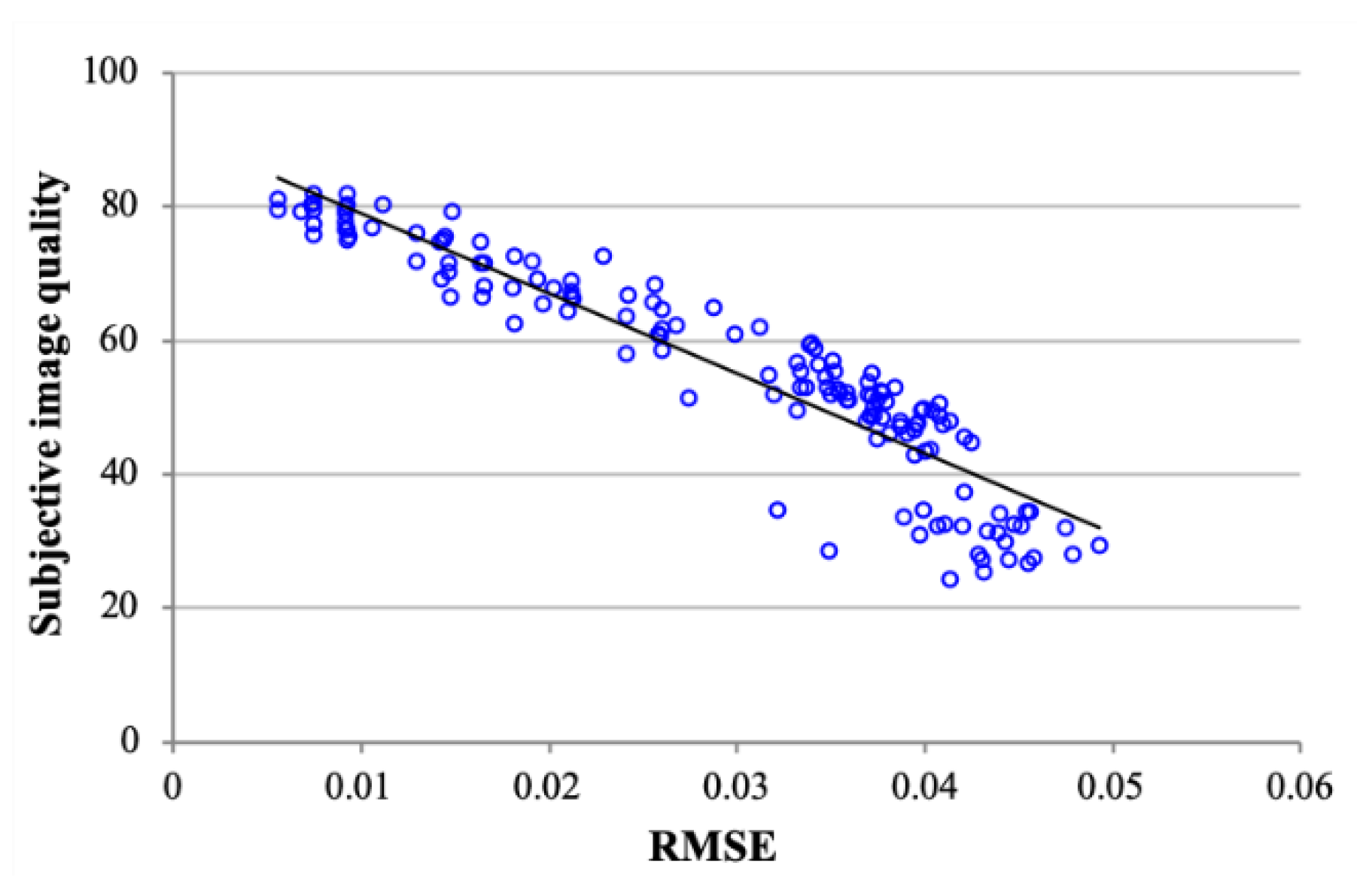
The relationship between the perceived image quality and the values of RMSE and SSIM is analyzed based on the LIVE Image Quality Assessment Database [29,30,31] released by Laboratory for Image and Video Engineering (LIVE) at University of Texas at Austin. This database provides the difference mean opinion scores (DMOS) of the subjective image quality ratings on 29 natural images with five types of distortions, including JPEG2000, JPEG, white Gaussian noise, Gaussian blur and Rayleigh fast-fading. The data was collected by performing a subjective experiment of image quality assessment according to the single-stimulus protocol. Participants in the experiment were asked to rate the quality of the images by ‘Bad’, ‘Poor’, ‘Fair’, ‘Good’ or ‘Excellent’. These ratings were translated into scores of 20, 40, 60, 80 and 100, respectively. Since the primary source of the noise generated by the IFTAs is the white Gaussian noise, we only used the results of the images distorted by this type of noise in this study. Five different degrees of white Gaussian noise were evaluated in the database. In total, there are 145 stimuli in total, excluding the 29 original images. The original images are assumed to have a perfect image quality. The RMSE and SSIM of these 145 stimuli with respect to their corresponding original images were calculated. Their relationships with the perceived image quality are plotted in Figure 6 and Figure 7. It can be seen that higher RMSE values are associated with poor image quality and higher SSIM values represent good image quality. SSIM values larger than 0.6 can always guarantee a good image quality while the corresponding boundary for RMSE is ~0.02. Linear relationships were observed in both figures. Linear fittings were applied to the results in these figures. Results show that SSIM has a more linear relationship with the perceived the image quality in the presence of white Gaussian noise than RMSE does. Since the images reconstructed from the phase-only holograms calculated by IFTAs are also distorted by the white Gaussian noise, SSIM is expected to be a reliable quality metric for the perceived image quality in IFTAs. In other words, we can use SSIM to evaluate the image reconstructed from phase-only holograms calculated by IFTAs.
5. Content Dependence of the Image Quality Metrics
Another advantage of SSIM over RMSE is its consistency over different images. In this work, GS algorithm was used generate the phase-only holograms corresponding to the 29 natural images in the LIVE Image Quality Assessment Database. A total of 400 GS iterations were carried out for each image. The large number of iterations used in this test is to ensure that all the reconstructed images have a good quality. The reconstructed images were evaluated by both RMSE and SSIM. Figure 8 shows the RMSE and SSIM values for the 29 reconstructed images.
It can be seen that the RMSE values ranges from <0.01 to >0.05 while the SSIM values are between 0.92 and 0.99. In other words, the absolute values of RMSE are more dependent on the image content instead of the image quality. Since the termination of IFTAs usually is determined by a predefined threshold of the image quality metric, it would be impossible to set a universal RMSE threshold value for IFTAs given its large dependence on the image content. As a result, the direct use of RMSE as the image quality metric in IFTAs would become much more complicated. In contrast, the limited spread of the SSIM values makes it a more consistent image quality metric in IFTAs.
6. Impact on the Speed of Hologram Generation
Although the image quality metrics do not affect the convergence speed of the IFTAs for the hologram generation, however, all the IFTAs rely on the image quality metrics to know when they should terminate the iterations, i.e., when further iterations would not yield improvement in the image quality, especially the perceived image quality.
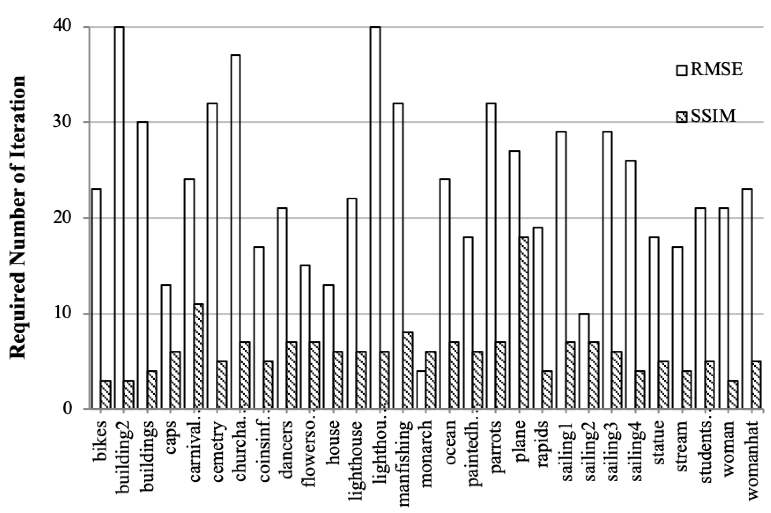
In the first test, the GS algorithms using the RMSE or SSIM as the image quality metrics were used to generate the phase-only holograms for the 29 natural images in the LIVE Image Quality Assessment Database. The algorithm would terminate when it reaches convergence, i.e., when the image quality metric varies less than 10% for the past ten consecutive iterations. The required number of iterations for each image were plotted in Figure 9 for both image quality metrics. It can be seen that the GS algorithm using SSIM as the image quality metric converges more quickly for 18 out of the 29 tested images than the same algorithm based on the RMSE. The same analysis was carried out for the Fienup and FiDOC algorithms based on RMSE and SSIM. The results were plotted in Figure 10 and Figure 11. For the Fienup algorithm, SSIM would terminate the iterations quicker for 24 out of the 29 tested images. For the FiDOC algorithm, the SSIM would terminate the iterations quicker for 28 out of the 29 tested images. It can be seen that the SSIM is able to terminate the iterations more quickly in all the three IFTAs.
Figure 12 plots the average number of iterations required in each IFTA configuration. For the 29 images tested in this study, the performance of GS and Fienup algorithms were similar when RMSE was used as the image quality metric. The use of SSIM reduced the number of required iterations in GS and Fienup algorithms by 25% and 50%, respectively. FiDOC algorithm was able to significantly improve the calculation speed on its own, which was consistent with previous results [18,19]. In addition to this, SSIM was able to further reduce the required number of iterations by 75% in the FiDOC algorithm, compared to when RMSE was used as the image quality metric.
The don’t-care area used in the FiDOC algorithm increases the dimensions of the image, which makes the calculation time for each iteration longer. Figure 13 plots the average calculation time for the 29 test images using different algorithm settings. The calculation was carried out in MATLAB 2019a on a Windows 10 PC with Intel i9-9820x processor and 128 GB RAM. When RMSE is used as the image quality metric, FiDOC algorithm is actually the slowest despite the minimal number of iterations required. When SSIM is used as the image quality metric, the reduction of the iteration number by the FiDOC algorithm can actually lead to improvement in the calculation speed.
In order to further validate the results, McGill Calibrated Colour Image Database [32] was used to compare the performance of FiDOC algorithm using RMSE or SSIM as the image quality metrics. This database contained over 1500 images, which made the results more representative. Figure 14 plots the average iterations among all the images using the two algorithm configurations under comparison. It can be seen that SSIM was able to reduce the required number of iterations by over two-thirds, when compared with the RMSE. This is consistent with results obtained based on the LIVE Image Quality Assessment Database in general.
It should be stressed again that the SSIM as an image quality metric does not speed up the IFTAs themselves. The extra iterations performed when RMSE was used as the image metric may still lead to improvement in the reconstruction quality in some cases. However, such improvement had little impact on the perceived image quality. Therefore, these extra iterations are not necessary. SSIM’s ability to predict the perceived image quality of reconstructed images consistently enabled IFTAs to terminate as early as possible. As a result, the required number of iterations for the IFTAs can be kept at the minimum.
7. Conclusions
This work has identified that the main distortion in the images reconstructed from the phase-only holograms calculated by IFTAs is the white Gaussian noise. The perceived quality of such images can be better evaluated by using SSIM instead of RMSE. As a result, the SSIM was proposed as the image quality metric in IFTAs in this work. To the authors’ knowledge, this is the first time that perceived image quality has been used as the quality metric in IFTAs. Moreover, SSIM also proves to be less dependent on the image content as the natural images with similar perceived quality always have comparable SSIM values. All these properties enable the IFTAs using SSIM as the image quality metric to terminate when further iterations would not lead to significant improvement in the perceived image quality. As a result, the required number of iterations can be kept as the minimum and calculation speed is improved. In particular, up to 75% of unnecessary iterations were eliminated in the FiDOC algorithm. When necessary, SSIM can also be used in conjunction with other metrics, e.g., peak signal-to-noise ratio, diffraction efficiency and uniformity error, to determine the best results for the target application.
Author Contributions
Conceptualization, H.Y. and D.C.; investigation, H.Y.; formal analysis, H.Y. and D.C.; writing-original draft preparation, H.Y.; writing-review and editing, H.Y. and D.C.
Funding
This research was funded by Fundamental Research Funds for the Central Universities (2242019k1G001).
Conflicts of Interest
The authors declare no conflict of interest.
References
- Collings, N.; Reufer, M.; Penty, R.V.; Sumpf, B.; Safer, M.; Chu, D.P.; Crossland, W.A. Holographic projection based on tapered lasers and nematic liquid crystal on silicon devices. In Proceedings of the SPIE Photonic Devices Applications, San Diego, CA, USA, 1–5 August 2010; p. 777504. [Google Scholar]
- Collings, N.; Davey, T.; Christmas, J.; Chu, D.; Crossland, B. The applications and technology of phase-only liquid crystal on silicon devices. J. Disp. Technol. 2011, 7, 112–119. [Google Scholar] [CrossRef]
- Barnes, T.H.; Eiju, T.; Matusda, K.; Ooyama, N. Phase-only modulation using a twisted nematic liquid crystal television. Appl. Opt. 1989, 28, 4845. [Google Scholar] [CrossRef] [PubMed]
- Georgiou, A.; Christmas, J.; Collings, N.; Moore, J.; Crossland, W.A. Aspects of hologram calculation for video frames. J. Opt. A Pure Appl. Opt. 2008, 10, 35302. [Google Scholar] [CrossRef]
- Chen, J.-S.; Smithwick, Q.; Chu, D. Implementation of shading effect for reconstruction of smooth layer-based 3D holographic images. In Proceedings of the SPIE Stereoscopic Displays and Applications XXIV, San Francisco, CA, USA, 3–7 February 2013; p. 86480R. [Google Scholar]
- Matoba, O.; Naughton, T.J.; Frauel, Y.; Bertaux, N.; Javidi, B. Real-time three-dimensional object reconstruction by use of a phase-encoded digital hologram. Appl. Opt. 2002, 41, 6187–6192. [Google Scholar] [CrossRef] [PubMed]
- O’Brien, D.C.; Mears, R.J.; Wilkinson, T.D.; Crossland, W.A. Dynamic holographic interconnects that use ferroelectric liquid-crystal spatial light modulators. Appl. Opt. 1994, 33, 2795. [Google Scholar] [CrossRef]
- Robertson, B.; Yang, H.; Redmond, M.M.; Collings, N.; Moore, J.R.; Liu, J.; Jeziorska-Chapman, A.M.; Pivnenko, M.; Lee, S.; Wonfor, A.; et al. Demonstration of Multi-Casting in a 1 × 9 LCOS Wavelength Selective Switch. J. Light. Technol. 2014, 32, 402–410. [Google Scholar] [CrossRef]
- Yang, H.; Robertson, B.; Chu, D. Crosstalk Reduction in Holographic Wavelength Selective Switches Based on Phase-only LCOS Devices. In Proceedings of the Optical Fiber Communication Conference, San Francisco, CA, USA, 9–13 March 2014; p. Th2A.23. [Google Scholar]
- Crossland, W.A.; Wilkinson, T.D.; Manolis, I.G.; Redmond, M.M.; Davey, A.B. Telecommunications Applications of LCOS Devices. Mol. Cryst. Liq. Cryst. 2002, 375, 1–13. [Google Scholar] [CrossRef]
- Crossland, W.; Manolis, I.; Redmond, M.; Tan, K.; Wilkinson, T.; Holmes, M.; Parker, T.; Chu, H.; Croucher, J.; Handerek, V.; et al. Holographic optical switching: The “ROSES” demonstrator. J. Light. Technol. 2000, 18, 1845–1854. [Google Scholar] [CrossRef]
- Ashkin, A.; Dziedzic, J.M.; Bjorkholm, J.E.; Chu, S. Observation of a single-beam gradient force optical trap for dielectric particles. Opt. Lett. 1986, 11, 288. [Google Scholar] [CrossRef]
- Leach, J.; Sinclair, G.; Jordan, P.; Courtial, J.; Padgett, M.J.; Cooper, J.; Laczik, Z.J. 3D manipulation of particles into crystal structures using holographic optical tweezers. Opt. Express 2004, 12, 220. [Google Scholar] [CrossRef]
- Dammann, H. Spectral characteristics of stepped-phase gratings. Optik 1979, 53, 409–417. [Google Scholar]
- Wyrowski, F.; Bryngdahl, O. Iterative Fourier-transform algorithm applied to computer holography. J. Opt. Soc. Am. A 1988, 5, 1058–1065. [Google Scholar] [CrossRef]
- Gerchber, R.W.; Saxton, W.O. A practical algorithm for the determination of the phase from image and diffraction plane pictures. Optik 1972, 35, 237–246. [Google Scholar]
- Fienup, J.R. Phase retrieval algorithms: A comparison. Appl. Opt. 1982, 21, 2758–2769. [Google Scholar] [CrossRef] [PubMed]
- Akahori, H. Spectrum leveling by an iterative algorithm with a dummy area for synthesizing the kinoform. Appl. Opt. 1986, 25, 802–811. [Google Scholar] [CrossRef]
- Wyrowski, F. Diffractive optical elements: Iterative calculation of quantized, blazed phase structures. J. Opt. Soc. Am. A 1990, 7, 961–969. [Google Scholar] [CrossRef]
- Engeldrum, P.G. A theory of image quality: The image quality circle. J. Imag. Sci. Technol. 2004, 48, 447–457. [Google Scholar]
- Chu, D.P.; Dowsett, M.G.; Cooke, G.A. Characterization of the noise in secondary ion mass spectrometry depth profiles. J. Appl. Phys. 1996, 80, 7104–7107. [Google Scholar] [CrossRef] [Green Version]
- Lehmann, E.L.; Casella, G. Theory of Point Estimation; Springer: New York, NY, USA, 1998; Volume 31. [Google Scholar]
- Kishk, S.; Javidi, B. Watermarking of three-dimensional objects by digital holography. Opt. Lett. 2003, 28, 167–169. [Google Scholar] [CrossRef]
- Wang, Z.; Bovik, A. Mean squared error: Love it or leave it? A new look at Signal Fidelity Measures. IEEE Signal Process. Mag. 2009, 26, 98–117. [Google Scholar] [CrossRef]
- Carlson, C.R.; Cohen, R.W. A simple psycho-physical model for predicting the visibility of displayed information. Proc. Soc. Inf. Disp. 1980, 21, 229–246. [Google Scholar]
- Qin, S.; Ge, S.; Teunissen, K.; Heynderickx, I.; Yin, H.; Xia, J.; Liu, L. P-37: Just Noticeable Difference of Image Attributes for Natural Images. SID Symp. Dig. Tech. Pap. 2007, 38, 326–329. [Google Scholar] [CrossRef]
- Yang, H.; Liu, L.; Tang, H.; Qin, S.; Yin, H.; Tu, Y.; Heynderickx, I. Relationship of Just Noticeable Difference (JND) in Black Level and White Level With Image Content. J. Disp. Technol. 2014, 10, 470–477. [Google Scholar] [CrossRef]
- Barten, P.G.J. Evaluation of subjective image quality with the square-root integral method. J. Opt. Soc. Am. A 1990, 7, 2024–2031. [Google Scholar] [CrossRef]
- Wang, Z.; Bovik, A.; Sheikh, H.; Simoncelli, E. Image Quality Assessment: From Error Visibility to Structural Similarity. IEEE Trans. Image Process. 2004, 13, 600–612. [Google Scholar] [CrossRef] [Green Version]
- Sheikh, H.R.; Wang, Z.; Cormack, L.; Bovik, A.C. Live Image Quality Assessment Database Release 2. 2005. Available online: http://www.live.ece.utexas.edu/research/quality/subjective.htm (accessed on 2 October 2019).
- Sheikh, H.R.; Sabir, M.F.; Bovik, A.C. A Statistical Evaluation of Recent Full Reference Image Quality Assessment Algorithms. Image Process. IEEE Trans. 2006, 15, 3440–3451. [Google Scholar] [CrossRef]
- Olmos, A.; Kingdom, F.A.A. A biologically inspired algorithm for the recovery of shading and reflectance images. Perception 2004, 33, 1463–1473. [Google Scholar] [CrossRef]
Figure 1.
The image pattern used to analyze the noise characteristics in the image reconstructed from holograms calculated by iterative Fourier transform algorithms (IFTAs).
Figure 1.
The image pattern used to analyze the noise characteristics in the image reconstructed from holograms calculated by iterative Fourier transform algorithms (IFTAs).

Figure 2.
Reconstructed images after (a) 50; (b) 100; (c) 150; and (d) 200 Gerchberg–Saxton (GS) iterations.
Figure 2.
Reconstructed images after (a) 50; (b) 100; (c) 150; and (d) 200 Gerchberg–Saxton (GS) iterations.

Figure 3.
The distributions of grey values in the reconstructed images after (a) 50; (b) 100; (c) 150; and (d) 200 GS iterations.
Figure 3.
The distributions of grey values in the reconstructed images after (a) 50; (b) 100; (c) 150; and (d) 200 GS iterations.

Figure 4.
Reconstructed images from holograms calculated by (a) GS algorithm; (b) Fienup algorithm; and (c) ‘Fienup with don’t-care’ (FiDOC) algorithm, after 200 iterations.
Figure 4.
Reconstructed images from holograms calculated by (a) GS algorithm; (b) Fienup algorithm; and (c) ‘Fienup with don’t-care’ (FiDOC) algorithm, after 200 iterations.

Figure 5.
Distributions of grey values in the images reconstructed from holograms calculated by (a) GS algorithm; (b) Fienup algorithm; and (c) FiDOC algorithm, after 200 iterations.
Figure 5.
Distributions of grey values in the images reconstructed from holograms calculated by (a) GS algorithm; (b) Fienup algorithm; and (c) FiDOC algorithm, after 200 iterations.

Figure 6.
Relationship between the perceived image quality and root-mean-squared error (RMSE) values.
Figure 6.
Relationship between the perceived image quality and root-mean-squared error (RMSE) values.

Figure 7.
Relationship between the perceived image quality and structure similarity (SSIM) values.

Figure 8.
The RMSE and SSIM values of the reconstructed images after 200 GS iterations.

Figure 9.
The required number of iterations to reach the convergence for the GS algorithms based on RMSE and SSIM.
Figure 9.
The required number of iterations to reach the convergence for the GS algorithms based on RMSE and SSIM.

Figure 10.
The required number of iterations to reach the convergence for the Fienup algorithms based on RMSE and SSIM.
Figure 10.
The required number of iterations to reach the convergence for the Fienup algorithms based on RMSE and SSIM.

Figure 11.
The required number of iterations to reach the convergence for the FiDOC algorithms based on RMSE and SSIM.
Figure 11.
The required number of iterations to reach the convergence for the FiDOC algorithms based on RMSE and SSIM.

Figure 12.
The average number of iterations required for GS, Fienup and FiDOC algorithms based on RMSE and SSIM.
Figure 12.
The average number of iterations required for GS, Fienup and FiDOC algorithms based on RMSE and SSIM.

Figure 13.
The average calculation time required for GS, Fienup and FiDOC algorithms based on RMSE and SSIM.
Figure 13.
The average calculation time required for GS, Fienup and FiDOC algorithms based on RMSE and SSIM.

Figure 14.
The average calculation time required for FiDOC algorithm using RMSE or SSIM as the image quality metrics, based on the McGill Calibrated Colour Image Database.
Figure 14.
The average calculation time required for FiDOC algorithm using RMSE or SSIM as the image quality metrics, based on the McGill Calibrated Colour Image Database.


Table 1.
The fitted values in the grey value distribution models for the images reconstructed from the phase-only holograms calculated by GS algorithm with different numbers of iterations.
Table 1.
The fitted values in the grey value distribution models for the images reconstructed from the phase-only holograms calculated by GS algorithm with different numbers of iterations.
| Coefficients | Number of Iterations | |||
|---|---|---|---|---|
| 50 | 100 | 150 | 200 | |
| a1 | 6087.9 | 9317.1 | 12,103.0 | 14,522.3 |
| a2 | 11,365.6 | 17,663.8 | 22,999.3 | 27,765.5 |
| a3 | 5588.5 | 8684.9 | 11,338.1 | 13,765.3 |
| μ1 | 66.1 | 65.4 | 65.1 | 64.9 |
| μ2 | 127.8 | 127.9 | 127.9 | 127.9 |
| μ3 | 190.2 | 190.8 | 191.1 | 191.2 |
| δ1 | 6.1 | 4.0 | 3.1 | 2.5 |
| δ2 | 6.5 | 4.2 | 3.2 | 2.7 |
| δ3 | 6.6 | 4.3 | 3.3 | 2.7 |
| r2 | 0.99981 | 0.99990 | 0.99993 | 0.99995 |
Table 2.
The fitted values in the grey value distribution models for the images reconstructed from phase-only holograms calculated by GS, Fienup and FiDOC algorithms after 200 iterations.
Table 2.
The fitted values in the grey value distribution models for the images reconstructed from phase-only holograms calculated by GS, Fienup and FiDOC algorithms after 200 iterations.
| Coefficients | GS | Fienup | FiDOC |
|---|---|---|---|
| a1 | 14,522.33 | 21,265.85 | 22,270.95 |
| a2 | 27,765.50 | 40,998.93 | 41,226.04 |
| a3 | 13,765.31 | 20,282.40 | 20,691.99 |
| μ1 | 64.90 | 64.53 | 64.57 |
| μ2 | 127.93 | 127.95 | 127.94 |
| μ3 | 191.21 | 191.56 | 191.53 |
| δ1 | 2.55 | 1.74 | 1.66 |
| δ2 | 2.67 | 1.80 | 1.79 |
| δ3 | 2.68 | 1.83 | 1.79 |
| r2 | 0.99995 | 0.99996 | 0.99998 |
© 2019 by the authors. Licensee MDPI, Basel, Switzerland. This article is an open access article distributed under the terms and conditions of the Creative Commons Attribution (CC BY) license (http://creativecommons.org/licenses/by/4.0/).
Share and Cite
MDPI and ACS Style
Yang, H.; Chu, D. Iterative Phase-Only Hologram Generation Based on the Perceived Image Quality. Appl. Sci. 2019, 9, 4457. https://doi.org/10.3390/app9204457
AMA Style
Yang H, Chu D. Iterative Phase-Only Hologram Generation Based on the Perceived Image Quality. Applied Sciences. 2019; 9(20):4457. https://doi.org/10.3390/app9204457
Chicago/Turabian StyleYang, Haining, and Daping Chu. 2019. "Iterative Phase-Only Hologram Generation Based on the Perceived Image Quality" Applied Sciences 9, no. 20: 4457. https://doi.org/10.3390/app9204457
Note that from the first issue of 2016, this journal uses article numbers instead of page numbers. See further details here.