New Hybrid Algorithms for Prediction of Daily Load of Power Network

Abstract

Two new hybrid algorithms are proposed to improve the performances of the meta-heuristic optimization algorithms, namely the Grey Wolf Optimizer (GWO) and Shuffled Frog Leaping Algorithm (SFLA). Firstly, it advances the hierarchy and position updating of the mathematical model of GWO, and then the SGWO algorithm is proposed based on the advantages of SFLA and GWO. It not only improves the ability of local search, but also speeds up the global convergence. Secondly, the SGWOD algorithm based on SGWO is proposed by using the benefit of differential evolution strategy. Through the experiments of the 29 benchmark functions, which are composed of the functions of unimodal, multimodal, fixed-dimension and composite multimodal, the performances of the new algorithms are better than that of GWO, SFLA and GWO-DE, and they greatly balances the exploration and exploitation. The proposed SGWO and SGWOD algorithms are also applied to the prediction model based on the neural network. Experimental results show the usefulness for forecasting the power daily load.

1. Introduction

Global optimization problems are common in engineering, economics and many sciences, and that their general formulation is as in the equations below.

$$optimize\overrightarrow{x}\in f_j\left(x\right),(j=1,2,...,m)$$

(1)

$$\overrightarrow{x}=(x_1,x_2,...,x_n)$$

(2)

$$\overrightarrow{l}\le \overrightarrow{x}\le \overrightarrow{u}$$

(3)

where $\overrightarrow{l}$=($l_1$,$l_2$,...,$l_n$), $\overrightarrow{u}$=($u_1$,$u_2$,...,$u_n$). $\overrightarrow{x}$ is a decision vector, and n is the dimension of $\overrightarrow{x}$. The area covered by the decision vectors is called the search range. $\overrightarrow{u}$ and $\overrightarrow{l}$ are the upper and lower bounds of the search range, and they also have n dimensions. $f_j\left(x\right)$ is called the cost or fitness function. If m equals 1, $f_1\left(x\right)$ is a single fitness function. In the paper, it only considers a single objective, so $f_1\left(x\right)$ is described as $f\left(x\right)$.

The meta-heuristic algorithm is an improvement of the heuristic algorithm and it adopts the methods of local search and stochastic, which provides a solution to an acceptance of optimization problem to some extent. Meta-heuristic is an iterative process. Through the combination of different concepts, the process uses the algorithm to exploration and exploitation in the search range. Learning strategy is used to acquire and master information to find the approximate optimal solution during the process. The algorithm is an effective way to solve global optimization problems, and it has the characteristics of generality, stability, and fast convergence. It includes two criteria, exploration and exploitation. Exploitation reflects the ability of finding the best around a good range, while exploration reflects the ability of searching for new range. At the beginning, it should search the whole range as much as possible, then through using exploitation it searches more carefully around the good solution. But they are contradictory. Too small exploration leads to convergence too fast and easy falling into local optimum; however, too small exploitation makes the algorithm converge too slowly.

The No Free Lunch (NFL) theorem considers that there is no meta-heuristic algorithm applying for all optimization problems [1,2]. In other words, an algorithm shows very promising results on a set of issues, but it doesn’t perform well on another set of issues. So it needs putting forward a new algorithm to get high performance in certain specific areas.

Over the past decades, a large number of meta-heuristics are inspired by natural behaviors [3,4,5], such as, Genetic Algorithm (GA) [6,7,8], Differential Evolution (DE) Algorithm [9,10,11,12], Grey Wolf Optimizer (GWO) Algorithm [13,14,15,16,17], Particle Swarm Optimization (PSO) Algorithm [18,19,20,21], Artificial Bee Colony (ABC) Algorithm [22,23,24], Cat Swarm Optimization (CSO) [25,26,27], Artificial Fish Swarm Algorithm (AFSA) [28,29], Ant Colony Optimization (ACO) Algorithm [30,31,32,33,34], Shuffled Frog Leaping Algorithm (SFLA) [35,36,37,38,39,40], Biogeography Based Optimization (BBO) Algorithm [41,42,43], QUasi-Affine TRansformation Evolutionary (QUATRE) Algorithm [44,45,46,47] and so on. Because they all have some defects, many researchers also introduce hybrid algorithms to improve the defects [48,49,50,51,52,53,54,55].

The rest of the paper is organized as follows: some related research works are described in the Section 2. Section 3 improves the model of GWO, and then puts forward two algorithms, SGWO and SGWOD. Section 4 testifies the performances of GWO, GWO-DE, SFLA, SGWO and SGWOD by 29 benchmark functions. Section 5 uses the algorithms to predict daily power load based on the neural network. Finally, it concludes the works of the paper and gives some advice to go on work.

2. Related Research Works

In the section, it briefly reviews the basic theories of Grey Wolf Optimizer (GWO), Differential Evolution (DE) and Shuffled Frog Leaping Algorithm (SFLA). GWO and SFLA are swarm intelligence algorithms, and DE is a heuristic random search algorithm based on group difference.

2.1. Grey Wolf Optimizer

GWO mimics the behaviors of grey wolf, such as social hierarchy, searching and hunting prey [13]. Each wolf represents a candidate solution to the problem to be solved, and the prey represents the optimal to be found. GWO refers to the first three optimal solutions respectively named alpha ($\alpha$), beta ($\beta$) and delta ($\delta$). The remaining candidates are collectively referred to as omega ($\omega$). Based on the locations of the three optimal solutions, the omegas can update their positions. GWO has the characteristics of strong convergence, few parameters and easy realization.

The wolf’s position is expressed as follows:

$$\overrightarrow{D}=|\overrightarrow{B}·\overrightarrow{X_p}\left(t\right)-\overrightarrow{X_i}\left(t\right)|$$

(4)

$$\overrightarrow{X_i}(t+1)=\overrightarrow{X_i}\left(t\right)-\overrightarrow{A}·\overrightarrow{D}$$

(5)

where $\overrightarrow{X_i}$ and $\overrightarrow{X_p}$ are the position vectors of i and prey, respectively; t represents the current iteration; both $\overrightarrow{A}$ and $\overrightarrow{B}$ are coefficient vectors, which are calculated as follows:

$$\overrightarrow{A}=2\overrightarrow{a}·\overrightarrow{r_1}-\overrightarrow{a}$$

(6)

$$\overrightarrow{B}=2\overrightarrow{r_2}$$

(7)

With the iteration process, a linearly decreases from 2 to 0. $\overrightarrow{r_1}$ and $\overrightarrow{r_2}$ are random vectors between [0, 1].

During hunting, the alpha, beta and delta guides the wolf pack. A wolf first computes its distance to them according to Equations (8) and (9), and then updates its position by Equation (10).

$$\overrightarrow{D_{\alpha }}=|\overrightarrow{B_1}·\overrightarrow{X_{\alpha }}-\overrightarrow{X_i}|,\overrightarrow{D_{\beta }}=|\overrightarrow{B_2}·\overrightarrow{X_{\beta }}-\overrightarrow{X_i}|,\overrightarrow{D_{\delta }}=|\overrightarrow{B_3}·\overrightarrow{X_{\delta }}-\overrightarrow{X_i}|$$

(8)

$$\overrightarrow{X_1}=\overrightarrow{X_{\alpha }}-\overrightarrow{A_1}·\overrightarrow{D_{\alpha }},\overrightarrow{X_2}=\overrightarrow{X_{\beta }}-\overrightarrow{A_2}·\overrightarrow{D_{\beta }},\overrightarrow{X_3}=\overrightarrow{X_{\delta }}-\overrightarrow{A_3}·\overrightarrow{D_{\delta }}$$

(9)

$$\overrightarrow{X_i}(t+1)={\displaystyle \frac{\overrightarrow{X_1}+\overrightarrow{X_2}+\overrightarrow{X_3}}{3}}$$

(10)

where $\overrightarrow{X_{\alpha }}$, $\overrightarrow{X_{\beta }}$ and $\overrightarrow{X_{\delta }}$ respectively represent the positions of $\alpha$, $\beta$ and $\delta$. $\overrightarrow{D_{\alpha }}$, $\overrightarrow{D_{\beta }}$ and $\overrightarrow{D_{\delta }}$ respectively represent the distances between $\alpha$, $\beta$, $\delta$ and i.

Figure 1 shows the complete flow chart of GWO. It randomly initializes the wolf pack in a limited space and calculates the fitness of each wolf. Then it selects the top three best wolves to update the positions of the wolves according to the Equations (8) to (10), and finally outputs the optimal.

2.2. Differential Evolution

Like other evolutionary algorithms, DE operates on the candidate solutions of the population [9], but the population reproduction is different from others. The evolutionary process of DE contains three operations, $mutation$, $crossover$ and $selection$, which is very similar to GA. It preserves the individual optimal and shares the information with the population, that is, the optimization problem is solved through cooperation and competition among individuals.

A new individual is produced through adding the differences between two individuals to another, called $mutation$. The new one is compared with the individuals in the current population, called $crossover$; if its fitness is better, the old individual will be replaced by it in the next generation, otherwise the old one is still preserved, which is called $selection$. It evaluates the optimal of each generation during the evolution process. But in the process of solving problems, DE may lead to decrease the diversity of the population and cause the algorithm to stagnate.

It randomly selects two different individuals in the population, then amplifies the difference and performs synthesis with the mutated one. For each objective $x_i\left(t\right)$, Equation (11) generates a mutant.

$$m_i(t+1)=x_{r_1}\left(t\right)+\lambda \ast (x_{r_2}\left(t\right)-x_{r_3}\left(t\right))$$

(11)

where $x_{r_1}\left(t\right)$ denotes the individual $r_1$ in the $t^{th}$ generator. $r_1$, $r_2$ and $r_3$ are different individuals, which are randomly selected from the population. $\lambda$ is a constant factor between [0, 2] and it is used to control the proportion of the differential variation ($x_{r_2}\left(t\right)-x_{r_3}\left(t\right)$).

A new trial is generated by crossover operation and it increases the diversity of the population. It is produced as following:

$$c_{i,j}(t+1)=\left\{\begin{array}{c}{m}_{i,j}(t+1)if(rand\left(j\right)\le pCR)orj=randi\left(i\right)\hfill \\ x_{i,j}(t+1)if(rand\left(j\right)>pCR)orj!=randi\left(i\right)\hfill \end{array}\right.$$

(12)

where $rand\left(j\right)$ is a random constant between [$0,1$] and $pCR$ is a crossover constant between [$0,1$]. $randi\left(i\right)$ is a randomly chosen integer between [$1,n$]; j is the dimension of an individual.

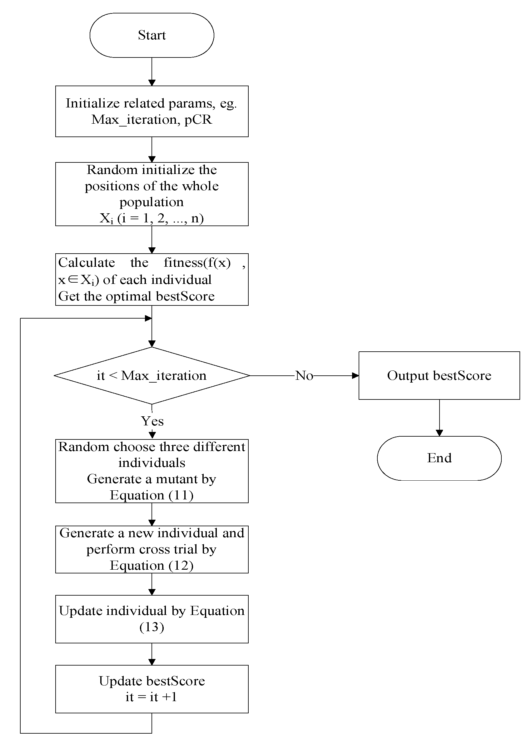
According to Equation (13), if $c_i(t+1)$ is better than $x_i\left(t\right)$, it will replace $x_i$ in the ${(t+1)}^{th}$ generation. Figure 2 shows the complete flow chart of DE. It randomly initializes the population and calculates the fitness of each individual. Then it generates a new individual through random selecting three ones to perform mutation and crossover, and it determines whether to replace the original with the new one by Equation (13). Finally it outputs the optimal.

$$x_i(t+1)=\left\{\begin{array}{c}{c}_i(t+1)if(f\left(c_i(t+1)\right)<f\left(x_i\left(t\right)\right))\hfill \\ x_i\left(t\right)else\hfill \end{array}\right.$$

(13)

2.3. Shuffled Frog Leaping Algorithm

SFLA utilizes the shuffled complex evolution strategy, which is a post-heuristic computing [35]. A group of frogs are divided into several subgroups. Different subgroups are considered to be a collection of frogs with different ideas and each subgroup is allowed to independently develop. After several evolutions, the all subgroups are reunited. It has the functions of global information exchange and local search, which achieves the balance between local search and global search.

Firstly, the frogs are sorted in descending order according to their fitness. Supposed the whole population consists of m memeplexes and each contains n frogs, so it satisfies the relationship $N=m\times n$. The first, second and $m^{th}$ frogs are divided into the first, second and $m^{th}$ memeplexes respectively. Then the ${(m+1)}^{th}$ frog is reassigned to the first memeplex, and so on. Figure 3 shows the memeplex partitioning process. Where the 1st, ${(m+1)}^{th}$, …, ${((n-1)\ast m+1)}^{th}$ frogs are divided into the 1st memeplex and the $m^{th}$, ${(m+m)}^{th}$, …, ${(n\ast m)}^{th}$ frogs are divided into the $m^{th}$ memeplex.

$X_a$ is the best frog in the population, while $X_z$ and $X_p$ respectively represent the worst and best frogs of each memeplex. Each memeplex performs local search, and the position of the frog is updated as follows:

$$X=\ell ·(X_p-X_z)$$

(14)

$$X_z^{\prime }=X_z+X,\left|\right|X\left|\right|\le X_m$$

(15)

$$X=\ell ·(X_a-X_z)$$

(16)

where ℓ is a random factor between [0 1]. $X_m$ indicates the maximum value that the frog is allowed to change position. If $X_z^{\prime }$ is better than $X_z$, the latter is replaced by the former. Otherwise, $X_a$ replaces $X_p$ and it continues to calculate $X_z^{\prime }$ by Equations (15) and (16). If it still hasn’t improved, $X_z$ is replaced by a random position. When the local search is completed, the frogs in all memeplexes are combined and sorted, then they are divided into memeplexs to continue to do local search. Figure 4 and Figure 5 show the whole flow chart of SFLA. It randomly initializes the frog group, calculates the fitness of each frog and sorts the frogs by the fitness. The group is divided into different meme groups to execute sub-processes. After the sub-processes are executed, all frogs are merged and sorted again, and then the sub-processes are re-executed until the algorithm ends and it outputs the optimal. During the sub-process, it updates the frogs in the worst position by Equations (14) to (16).

3. New Hybrid Algorithms Based on GWO, SFLA and DE

GWO has a great performance in convergence, but it’s easy to fall into the trap of local optimum. While SFLA has a great outstanding in global search, but its convergence is unsatisfactory. In the section, a new hybrid algorithm SGWO, based on GWO and SFLA, is proposed to overcome their defects. In a biological community, the species with the worst adaptability tend to be eliminated, or they must have to gain greater viability through variation. SGWOD draws the learning strategies from SGWO and DE to get better performance.

3.1. Advanced the Model of GWO

Before starting to design the hybrid algorithms, we first modify the mathematical model of GWO. When the fitness of the alpha is not as good as a new wolf, the former is replaced by the latter. But the old alpha may also have some important information, so it needs proposing a new hierarchy model to utilize the experience of the old one. By Equation (10), we know that it doesn’t consider the different importance of the alpha, beta and delta on guiding attack, so a new position updating model is introduced.

3.1.1. A New Hierarchy Model

The alpha is responsible for directing the wolf pack during hunting. Although it has great power, it is responsible for the safety and the livelihood of the wolves, and it is also under the supervision of the pack. There is not inheritance to the position of the alpha, and it needs accepting the challenges of other wolves. If it is defeated, the winner becomes the new leader (new alpha). The beta and delta are usually composed of experienced members of the wolves, which assist the alpha to complete the hunting. Once the alpha can’t lead the wolf pack to capture prey well, they replace it.

The new mathematical model is established based on the above descriptions. If the alpha doesn’t lead the wolf pack to catch prey well, it degenerates into the beta, and it doesn’t directly turn into an omega. The updating equations of the alpha are defined as follows:

$$\alpha \left(t\right)\to \left\{\begin{array}{c}\beta \left(t\right)if\left(f\right(\alpha \left(t\right))>f(i\left(t\right)\left)\right)\hfill \\ \alpha \left(t\right)else\hfill \end{array}\right.$$

(17)

$${\alpha }^{\prime }\left(t\right)=i\left(t\right)if(f\left(\alpha \left(t\right)\right)>f\left(i\left(t\right)\right))$$

(18)

where i represents a candidate solution; t indicates the current iteration; f is the fitness function; ${\alpha }^{\prime }$ means the new alpha.

If the beta hunts better than i, it is not replaced by i. But if it does not good at assisting the alpha, it becomes the delta and it doesn’t turn into an omega wolf. The beta is updated as follows:

$$\beta \left(t\right)\to \left\{\begin{array}{c}\delta \left(t\right)if\left(f\right(\beta \left(t\right))>f(i\left(t\right)\left)\right)\hfill \\ \beta \left(t\right)else\hfill \end{array}\right.$$

(19)

$${\beta }^{\prime }\left(t\right)=i\left(t\right)if(f\left(\beta \left(t\right)\right)>f\left(i\left(t\right)\right))$$

(20)

where ${\beta }^{\prime }\left(t\right)$ represents the new beta.

If the delta hunts better than i, it will not be replaced by i. But if it performs bad in hunting, it becomes an omega. The updating equations of the delta are defined as follows:

$$\delta \left(t\right)\to \left\{\begin{array}{c}\delta \left(t\right)if\left(f\right(\delta \left(t\right))>f(i\left(t\right)\left)\right)\hfill \\ \omega \left(t\right)else\hfill \end{array}\right.$$

(21)

$${\delta }^{\prime }\left(t\right)=i\left(t\right)if(f\left(\beta \left(t\right)\right)>f\left(i\left(t\right)\right))$$

(22)

where ${\delta }^{\prime }\left(t\right)$ represents the new delta.

3.1.2. A New Position Updating Model

Supposed an integer sequence $R=\{1,2,\dots ,i,\dots ,n\}$, $R_i$ represents the probability of i. If it follows a triangular discrete distribution, so the $i^{th}$ in the sequence has the following probability.

$$P_i={\displaystyle \frac{2i}{n(n+1)}}$$

(23)

The wolves work together in hunting, that the alpha leads the pack to attack prey and the beta and delta assist it to complete the attack. Therefore, the alpha plays a decisive role in the position updating of the pack, while the beta and delta play an auxiliary roles. But when the wolves update their positions, the Equation (10) doesn’t consider the decisive roles of the alpha, beta, and delta. The fitness is sorted from good to bad, then a new position equation is proposed as follows.

$$P_i={\displaystyle \frac{2(n+1-i)}{n(n+1)}}$$

(24)

$$X={\displaystyle \frac{\begin{array}{c}{\sum }_{i=1}^3{P}_i{X}_i\end{array}}{\begin{array}{c}{\sum }_{i=1}^3{P}_i\end{array}}}$$

(25)

where $P_i$ represents the importance of $X_i$ and i is selected from the alpha, beta and delta.

3.2. Hybrid Algorithm SGWO

From the position updating equations we have known that GWO makes all members converge quickly towards the optimal, while SFLA only makes the worst members converge to the optimum. But GWO may fall into local optimum due to too fast convergence, SFLA achieves global information exchange by combining memeplexes, which avoids local convergence. So through combining two or more methods, the hybrid algorithm effectively solves the problems. The process of SGWO is described as follows:

Step 1. Sort the population by fitness.

Step 2. Divide the population into different meme groups.

Step 3. Perform the following local search for each meme group.

  Step 3.1. Find the alpha, beta and delta.

  Step 3.2. Access each wolf and update the alpha, beta and delta by Equations (17)–(22).

  Step 3.3. Update the position of each wolf by Equation (25).

  Step 3.4. Repeatedly do 3.1–3.3 until it meets the ending conditions of local search.

Step 4. Combine the meme groups and repeatedly do 1–3 until it meets the ending conditions of the algorithm.

The pseudo code of SGWO is described in Algorithm 1.

Algorithm 1 SGWO

Initialize related parameters Initialize the positions of the population Calculate the fitness of each wolf nPop = the number of the population n_Memeplex = the number of Memeplex I = reshape(1:nPop, n_Memeplex, []); for$i=1:Max\_iteration$do  memes = cell(n_Memeplex, 1);  Sort the population by fitness  for $k=1:n\_Memeplex$ do   memesk = pop(I(k,:));   memesk = RunSGWO(parameters);   pop(I(k,:)) = memesk;  end for end for

The pseudo code of RunSGWO function is described in Algorithm 2.

Algorithm 2 RunSGWO

Find the alpha, beta and delta. for$i=1:Max\_iteration$do  for $s=1:subPopSize$ do   flag = 1;   fitness = fobj(pop(s).Position);   if fitness < alpha then    beta = alpha;    alpha = pop(s);    flag = 0;   end if   if $fitness<beta\&\&flag==1$ then    delta = beta;    beta = pop(s);    flag = 0;   end if   if $fitness<delta\&\&flag==1$ then    beta = pop(s);   end if   Update the position of s by Equation (25)   Calculate the fitness of s  end for end for

3.3. Hybrid Algorithm SGWOD

Gene mutation occurs in the organism when a creature breeds its next generation. If the mutation is beneficial to the organism, the variants are filtered through the environment and mutant genes are preserved in offspring. After each iteration, the wolves of a memeplex are updated by DE. That is, it eliminates the wolves with the worst fitness. At the same time, new ones are generated to replace the eliminated. The process of SGWOD is described as follows:

Step 1. Sort the population by fitness.

Step 2. Divide the population into different meme groups.

Step 3. Perform the following local search for each meme group.

  Step 3.1. Find the alpha, beta and omega.

  Step 3.2. Access each wolf and update the alpha, beta and omega by Equations (17)–(22).

  Step 3.3. Update the position of each wolf by Equation (25).

  Step 3.4 Access each wolf, randomly mutate and cross, if the new mutant is better than the old, it is replaced by the new one.

  Step 3.5. Repeatedly do 3.1–3.4 until it meets the ending conditions of the local search.

Step 4. Combine the meme groups and repeatedly do 1–3 until it meets the ending conditions of the algorithm.

4. Experiments and Results

In the section, we use 29 benchmark functions to test. These classical functions, listed in

Table 1. Unimodal benchmark functions.

Function	Space	D${}_{\mathit{i}\mathit{m}}$	${\mathbf{f}}_{\mathbf{min}}$
$f_1\left(x\right)={\sum }_{i=1}^n{x}_i^2$	[−100, 100]	30	0
$f_2\left(x\right)={\sum }_{i=1}^n|x_i|+{\prod }_{i=1}^n\left|x_i\right|$	[−10, 10]	30	0
$f_3\left(x\right)={\sum }_{i=1}^n{\left({\sum }_{j-1}^i{x}_j\right)}^2$	[−100, 100]	30	0
$f_4\left(x\right)=ma{x}_i\left\{\right|x_i|,1\le i\le n\}$	[−100, 100]	30	0
$f_5\left(x\right)={\sum }_{i=1}^{n-1}[100{(x_{i+1}-x_i^2)}^2+{(x_i-1)}^2]$	[−30, 30]	30	0
$f_6\left(x\right)={\sum }_{i=1}^n{\left([x_i+0.5]\right)}^2$	[−100, 100]	30	0
$f_7\left(x\right)={\sum }_{i=1}^{n}i{x}_i^4+random[0,1)$	[−1.28, 1.28]	30	0

,

Table 2. Multimodal benchmark functions.

Function	Space	D${}_{\mathit{i}\mathit{m}}$	${\mathbf{f}}_{\mathbf{min}}$
$f_8\left(x\right)={\sum }_{i=1}^n-x_{i}sin\left(\sqrt{|x_i|}\right)$	[−500, 500]	30	−12,569
$f_9\left(x\right)={\sum }_{i=1}^n[x_i^2-10cos\left(2\pi x_i\right)+10]$	[−5.12, 5.12]	30	0
$f_{10}\left(x\right)=-20exp(-0.2\sqrt{{\displaystyle \frac{1}{n}}{\sum }_{i=1}^n{x}_i^2})-exp({\displaystyle \frac{1}{n}}{\sum }_{i=1}^n$ $cos\left(2\pi x_i\right))+20+e$	[−32, 32]	30	0
$f_{11}\left(x\right)={\displaystyle \frac{1}{4000}}{\sum }_{i=1}^n{x}_i^2-{\prod }_{i=1}^{n}cos\left({\displaystyle \frac{x_i}{\sqrt{i}}}\right)+1$	[−600, 600]	30	0
$f_{12}\left(x\right)={\displaystyle \frac{\pi }{n}}\{10sin\left(\pi y_1\right)+{\sum }_{i=1}^{n-1}{(y_i-1)}^2[1+10si{n}^2(\pi$ $y_{i+1}\left)\right]+{(y_n-1)}^2\}+{\sum }_{i=1}^{n}u(x_i,10,100,4)$ $y_i=1+{\displaystyle \frac{x_i+1}{4}}u(x_i,a,k,m)=\left\{\begin{array}{c}k{(x_i-a)}^m{x}_i>a\hfill \\ 0-a<x_i<a\hfill \\ k{(-x_i-a)}^m{x}_i<-a\hfill \end{array}\right.$	[−50, 50]	30	0
$f_{13}\left(x\right)=0.1\{si{n}^2\left(3\pi x_1\right)+{\sum }_{i=1}^n{(x_i-1)}^2[1+si{n}^2(3\pi x_i$ $+1\left)\right]+{(x_n-1)}^2[1+si{n}^2\left(2\pi x_n\right)]\}+{\sum }_{i=1}^{n}u(x_i,10,100,4)$	[−50, 50]	30	0

,

Table 3. Fixed-dimension multimodal benchmark functions.

Function	Space	D${}_{\mathit{i}\mathit{m}}$	${\mathbf{f}}_{\mathbf{min}}$
$f_{14}\left(x\right)={(\frac{1}{500}{\sum }_{j=1}^{25}{\displaystyle \frac{1}{j+{\sum }_{i=1}^2{(x_i-a_{ij})}^6}})}^{-1}$	[−65, 65]	2	1
$f_{15}\left(x\right)={\sum }_{i=1}^{11}{[a_i-{\displaystyle \frac{x_1(b_i^2+b_i{x}_2)}{b_i^2+b_i{x}_3+x_4}}]}^2$	[−5, 5]	4	0.00030
$f_{16}\left(x\right)=4x_1^2-2.1x_1^4+\frac{1}{3}{x}_1^6+x_1{x}_2-4x_2^2+4x_2^4$	[−5, 5]	2	−1.0316
$f_{17}\left(x\right)={(x_2-\frac{5.1}{4{\pi }^2}{x}_1^2+\frac{5}{\pi }{x}_1-6)}^2+10(1-\frac{1}{8\pi })cos{x}_1+10$	[−5, 5]	2	0.398
$f_{18}\left(x\right)=[1+{(x_1+x_2+1)}^2$ $(19-14x_1+3x_1^2-14x_2+6x_1{x}_2+3x_2^2)]$ $\times [30+{(2x_1-3x_2)}^2\times (18-32x_1+12x_1^2+48x_2$ $-36x_1{x}_2+27x_2^2\left)\right]$	[−2, 2]	2	3
$f_{19}\left(x\right)=-{\sum }_{i=1}^4{c}_{i}exp(-{\sum }_{j=1}^3{a}_{ij}{(x_j-p_{ij})}^2)$	[1, 3]	3	−3.86
$f_{20}\left(x\right)=-{\sum }_{i=1}^4{c}_{i}exp(-{\sum }_{j=1}^6{a}_{ij}{(x_j-p_{ij})}^2)$	[0, 1]	6	−3.32
$f_{21}\left(x\right)=-{\sum }_{i=1}^5{[(X-a_i){(X-a_i)}^T+c_i]}^{-1}$	[0, 10]	4	−10.1532
$f_{22}\left(x\right)=-{\sum }_{i=1}^7{[(X-a_i){(X-a_i)}^T+c_i]}^{-1}$	[0, 10]	4	−10.4028
$f_{23}\left(x\right)=-{\sum }_{i=1}^{10}{[(X-a_i){(X-a_i)}^T+c_i]}^{-1}$	[0, 10]	4	−10.5363

and

Table 4. Composite multimodal benchmark functions.

Function	Space	D${}_{\mathit{i}\mathit{m}}$	${\mathbf{f}}_{\mathbf{min}}$
$F_{24}\left(CF1\right)$ $f_1,f_2,f_3,...,f_{10}=SphereFunction$ $[{\sigma }_1,{\sigma }_2,{\sigma }_3,...,{\sigma }_{10}]=[1,1,1,...,1]$ $[{\lambda }_1,{\lambda }_2,{\lambda }_3,...,{\lambda }_{10}]=[5/100,5/100,5/100,...,5/100]$	[−5, 5]	30	0
$F_{25}\left(CF2\right)$ $f_1,f_2,f_3,...,f_{10}=Griewan{k}^{\prime }sFunction$ $[{\sigma }_1,{\sigma }_2,{\sigma }_3,...,{\sigma }_{10}]=[1,1,1,...,1]$ $[{\lambda }_1,{\lambda }_2,{\lambda }_3,...,{\lambda }_{10}]=[5/100,5/100,5/100,...,5/100]$	[−5, 5]	30	0
$F_{26}\left(CF3\right)$ $f_1,f_2,f_3,...,f_{10}=Griewan{k}^{\prime }sFunction$ $[{\sigma }_1,{\sigma }_2,{\sigma }_3,...,{\sigma }_{10}]=[1,1,1,...,1]$ $[{\lambda }_1,{\lambda }_2,{\lambda }_3,...,{\lambda }_{10}]=[1,1,1,...,1]$	[−5, 5]	30	0
$F_{27}\left(CF4\right)$ $f_1,f_2=Ackle{y}^{\prime }sFunction,f_3,f_4=Rastrigi{n}^{\prime }sFunction,$ $f_5,f_6=WeierstrassFunction,f_7,f_8=Griewan{k}^{\prime }sFunction$ $f_9,f_{10}=SphereFunction$ $[{\sigma }_1,{\sigma }_2,{\sigma }_3,...,{\sigma }_{10}]=[1,1,1,...,1]$ $[{\lambda }_1,{\lambda }_2,{\lambda }_3,...,{\lambda }_{10}]=$ $[5/32,5/32,1,1,5/0.5,5/0.5,5/100,5/100,5/100,5/100]$	[−5, 5]	30	0
$F_{28}\left(CF5\right)$ $f_1,f_2=Rastrigi{n}^{\prime }sFunction,f_3,f_4=WeierstrassFunction,$ $f_5,f_6=Griewan{k}^{\prime }sFunction,f_7,f_8=Ackle{y}^{\prime }sFunction$ $f_9,f_{10}=SphereFunction$ $[{\sigma }_1,{\sigma }_2,{\sigma }_3,...,{\sigma }_{10}]=[1,1,1,...,1]$ $[{\lambda }_1,{\lambda }_2,{\lambda }_3,...,{\lambda }_{10}]=$ $[1/5,1/5,5/0.5,5/0.5,5/100,5/100,5/32,5/32,5/100,5/100]$	[−5, 5]	30	0
$F_{29}\left(CF6\right)$ $f_1,f_2=Rastrigi{n}^{\prime }sFunction,f_3,f_4=WeierstrassFunction,$ $f_5,f_6=Griewan{k}^{\prime }sFunction,f_7,f_8=Ackle{y}^{\prime }sFunction$ $f_9,f_{10}=SphereFunction$ $[{\sigma }_1,{\sigma }_2,{\sigma }_3,...,{\sigma }_{10}]=[0.1,0.2,0.3,0.4,0.5,0.6,0.7,0.8,0.9,1]$ $[{\lambda }_1,{\lambda }_2,{\lambda }_3,...,{\lambda }_{10}]=[0.1\ast 1/5,0.2\ast 1/5,0.3\ast 5/0.5,0.4\ast 5/0.5,$ $0.5\ast 5/100,0.6\ast 5/100,0.7\ast 5/32,0.8\ast 5/32,0.9\ast 5/100,1\ast 5/100]$	[−5, 5]	30	0

, are used by many researchers [56,57]. $Space$ is the boundary of its search range, $D_{im}$ represents the dimension of the function, and $f_{min}$ indicates the optimum of it.

4.1. Experimental Results

For verifying the results, SGWO and SGWOD are compared to GWO, SFLA and GWO-DE, which is an improved GWO with differential evolution [55]. They run 100 times on each benchmark function, and the testing parameters are listed in

Table 5. Parameters setting of each algorithm.

Algorithm	Main Parameters Setting
GWO	$Population\_number=300,Max\_iteration=100$
GWO-DE	$Population\_number=300,Max\_iteration=100,pCR=0.01,\lambda =[0.02,0.08]$
SFLA	$Population\_number=300,Max\_iteration=100,memeplex=5,$ $Parents\_number=3,Sons\_number=3,Memeplex\_iteration=2$
SGWO	$Population\_number=300,Max\_iteration=100,memeplex=5,$ $Memeplex\_iteration=2$
SGWOD	$Population\_number=300,Max\_iteration=100,pCR=0.01,$ $\lambda =[0.02,0.08],memeplex=5,Memeplex\_iteration=2$

.

Table 6. The statistical results of the algorithms.

Function	SGWO		SGWOD		GWO		SFLA		GWO-DE
	AVG	STSD	AVG	STSD	AVG	STSD	AVG	STSD	AVG	STSD
$f_1$	$1.68\times {10}^{-38}$	$6.50\times {10}^{-38}$	$1.70\times {10}^{-38}$	$3.10\times {10}^{-38}$	$9.71\times {10}^{-8}$	$6.50\times {10}^{-38}$	$3.26\times {10}^4$	$1.14\times {10}^4$	$3.50\times {10}^{-10}$	$4.41\times {10}^{-10}$
$f_2$	$1.23\times {10}^{-21}$	$1.58\times {10}^{-21}$	$2.05\times {10}^{-21}$	$2.00\times {10}^{-21}$	$8.23\times {10}^{-4}$	$1.58\times {10}^{-21}$	$1.46\times {10}^{39}$	$6.50\times {10}^{39}$	$3.45\times {10}^{-5}$	$2.78\times {10}^{-5}$
$f_3$	$4.73\times {10}^{-7}$	$1.24\times {10}^{-6}$	$5.94\times {10}^{-5}$	$1.74\times {10}^{-4}$	$7.81\times {10}^{-1}$	$1.24\times {10}^{-6}$	$8.02\times {10}^4$	$1.71\times {10}^4$	$1.35\times {10}^{-1}$	$1.55\times {10}^{-1}$
$f_4$	$6.65\times {10}^{-15}$	$7.04\times {10}^{-15}$	$6.13\times {10}^{-15}$	$6.94\times {10}^{-15}$	$3.71\times {10}^{-2}$	$7.04\times {10}^{-15}$	$7.78\times {10}^1$	$4.71\times {10}^0$	$1.03\times {10}^{-2}$	$5.58\times {10}^{-3}$
$f_5$	$2.85\times {10}^1$	$2.13\times {10}^{-1}$	$2.62\times {10}^1$	$1.28\times {10}^{-1}$	$2.68\times {10}^1$	$8.37\times {10}^{-1}$	$9.09\times {10}^7$	$4.41\times {10}^7$	$2.64\times {10}^1$	$6.24\times {10}^{-1}$
$f_6$	$4.03\times {10}^{-1}$	$1.13\times {10}^{-1}$	$1.38\times {10}^{-4}$	$2.91\times {10}^{-5}$	$2.22\times {10}^{-1}$	$1.13\times {10}^{-1}$	$3.46\times {10}^4$	$1.10\times {10}^4$	$8.58\times {10}^{-5}$	$2.85\times {10}^{-5}$
$f_7$	$4.50\times {10}^{-3}$	$5.55\times {10}^{-3}$	$1.53\times {10}^{-3}$	$1.40\times {10}^{-3}$	$5.15\times {10}^{-3}$	$5.50\times {10}^{-3}$	$1.71\times {10}^9$	$8.32\times {10}^8$	$6.93\times {10}^{-3}$	$6.17\times {10}^{-3}$
$f_8$	$-1.34\times {10}^{20}$	$9.48\times {10}^{20}$	$-3.70\times {10}^{37}$	$2.21\times {10}^{38}$	$-6.50\times {10}^3$	$9.48\times {10}^{20}$	$-2.38\times {10}^{19}$	$5.87\times {10}^{19}$	$-6.93\times {10}^3$	$2.98\times {10}^3$
$f_9$	0	0	0	0	$1.51\times {10}^1$	0	$3.80\times {10}^2$	$2.51\times {10}^1$	$2.73\times {10}^0$	$5.37\times {10}^0$
$f_{10}$	$4.48\times {10}^{-15}$	$3.55\times {10}^{-16}$	$4.41\times {10}^{-15}$	$3.55\times {10}^{-16}$	$6.77\times {10}^{-5}$	$3.55\times {10}^{-16}$	$1.89\times {10}^1$	$1.73\times {10}^0$	$3.46\times {10}^{-6}$	$2.11\times {10}^{-6}$
$f_{11}$	0	0	$1.32\times {10}^{-4}$	$1.32\times {10}^{-3}$	$6.33\times {10}^{-3}$	0	$2.49\times {10}^2$	$1.13\times {10}^2$	$3.88\times {10}^{-3}$	$7.19\times {10}^{-3}$
$f_{12}$	$1.89\times {10}^{-2}$	$1.88\times {10}^{-2}$	$1.42\times {10}^{-5}$	$4.04\times {10}^{-6}$	$1.99\times {10}^{-2}$	$1.88\times {10}^{-2}$	$1.59\times {10}^8$	$1.07\times {10}^8$	$4.34\times {10}^{-6}$	$1.24\times {10}^{-6}$
$f_{13}$	$2.00\times {10}^{-1}$	$5.85\times {10}^{-2}$	$3.03\times {10}^{-3}$	$4.83\times {10}^{-3}$	$2.33\times {10}^{-1}$	$5.85\times {10}^{-2}$	$3.22\times {10}^8$	$1.71\times {10}^8$	$8.13\times {10}^{-3}$	$4.17\times {10}^{-2}$
$f_{14}$	$2.27\times {10}^0$	$2.08\times {10}^0$	$2.50\times {10}^0$	$6.53\times {10}^{-1}$	$1.42\times {10}^0$	$2.08\times {10}^0$	$9.98\times {10}^{-1}$	$9.77\times {10}^{-8}$	$1.40\times {10}^0$	$7.05\times {10}^{-1}$
$f_{15}$	$6.80\times {10}^{-4}$	$3.62\times {10}^{-4}$	$5.30\times {10}^{-4}$	$2.64\times {10}^{-4}$	$9.72\times {10}^{-4}$	$3.62\times {10}^{-4}$	$1.73\times {10}^{-3}$	$6.42\times {10}^{-4}$	$1.20\times {10}^{-3}$	$3.94\times {10}^{-3}$
$f_{16}$	$-1.03\times {10}^0$	$2.19\times {10}^{-7}$	$-1.03\times {10}^0$	$5.02\times {10}^{-9}$	$-1.03\times {10}^0$	$2.19\times {10}^{-7}$	$-1.03\times {10}^0$	$7.85\times {10}^{-7}$	$-1.03\times {10}^0$	$1.54\times {10}^{-8}$
$f_{17}$	$3.98\times {10}^{-1}$	$1.21\times {10}^{-4}$	$3.98\times {10}^{-1}$	$1.22\times {10}^{-7}$	$3.98\times {10}^{-1}$	$1.21\times {10}^{-4}$	$3.98\times {10}^{-01}$	$4.70\times {10}^{-9}$	$3.98\times {10}^{-1}$	$5.97\times {10}^{-7}$
$f_{18}$	$3.00\times {10}^0$	$4.59\times {10}^{-3}$	$3.00\times {10}^0$	$2.53\times {10}^{-5}$	$3.00\times {10}^0$	$4.59\times {10}^{-3}$	$3.00\times {10}^0$	$2.71\times {10}^{-7}$	$3.00\times {10}^0$	$6.36\times {10}^{-6}$
$f_{19}$	$-3.85\times {10}^0$	$1.01\times {10}^{-2}$	$-3.86\times {10}^0$	$4.74\times {10}^{-7}$	$-3.86\times {10}^0$	$1.01\times {10}^{-2}$	$-3.86\times {10}^0$	$3.39\times {10}^{-8}$	$-3.86\times {10}^0$	$3.47\times {10}^{-4}$
$f_{20}$	$-3.26\times {10}^0$	$6.81\times {10}^{-2}$	$-3.29\times {10}^0$	$5.03\times {10}^{-2}$	$-3.24\times {10}^0$	$6.81\times {10}^{-2}$	$-3.25\times {10}^0$	$5.93\times {10}^{-2}$	$-3.25\times {10}^0$	$6.34\times {10}^{-2}$
$f_{21}$	$-9.86\times {10}^0$	$5.78\times {10}^{-1}$	$-1.02\times {10}^1$	$1.63\times {10}^{-4}$	$-9.50\times {10}^0$	$5.78\times {10}^{-1}$	$-7.22\times {10}^0$	$3.29\times {10}^0$	$-1.00\times {10}^1$	$8.74\times {10}^{-1}$
$f_{22}$	$-1.00\times {10}^1$	$7.60\times {10}^{-1}$	$-1.03\times {10}^1$	$7.48\times {10}^{-1}$	$-1.03\times {10}^1$	$7.60\times {10}^{-1}$	$-9.38\times {10}^0$	$2.34\times {10}^0$	$-1.04\times {10}^1$	$7.39\times {10}^{-4}$
$f_{23}$	$-1.01\times {10}^1$	$6.40\times {10}^{-1}$	$-1.05\times {10}^1$	$1.73\times {10}^{-4}$	$-1.03\times {10}^1$	$6.40\times {10}^{-1}$	$-9.84\times {10}^0$	$2.15\times {10}^0$	$-1.05\times {10}^1$	$7.57\times {10}^{-4}$
$f_{24}$	$2.22\times {10}^1$	$7.23\times {10}^1$	$2.39\times {10}^0$	$1.11\times {10}^1$	$2.74\times {10}^0$	$2.11\times {10}^1$	$5.38\times {10}^1$	$1.64\times {10}^2$	$9.43\times {10}^{-1}$	$4.86\times {10}^0$
$f_{25}$	$3.60\times {10}^1$	$1.19\times {10}^2$	$1.55\times {10}^1$	$5.34\times {10}^1$	$2.08\times {10}^1$	$7.37\times {10}^1$	$6.66\times {10}^1$	$2.05\times {10}^2$	$2.16\times {10}^1$	$7.95\times {10}^1$
$f_{26}$	$6.12\times {10}^1$	$1.88\times {10}^2$	$2.98\times {10}^1$	$9.49\times {10}^1$	$2.67\times {10}^1$	$8.47\times {10}^1$	$1.09\times {10}^2$	$3.30\times {10}^2$	$2.67\times {10}^1$	$8.40\times {10}^1$
$f_{27}$	$8.89\times {10}^1$	$2.68\times {10}^2$	$8.74\times {10}^1$	$2.65\times {10}^2$	$6.53\times {10}^1$	$2.03\times {10}^2$	$1.01\times {10}^2$	$3.06\times {10}^2$	$6.22\times {10}^1$	$1.96\times {10}^2$
$f_{28}$	$2.18\times {10}^1$	$6.83\times {10}^1$	$4.36\times {10}^0$	$1.57\times {10}^1$	$4.00\times {10}^0$	$1.52\times {10}^1$	$6.78\times {10}^1$	$2.10\times {10}^2$	$2.37\times {10}^0$	$1.18\times {10}^1$
$f_{29}$	$9.00\times {10}^1$	$2.71\times {10}^2$	$9.00\times {10}^1$	$2.71\times {10}^2$	$9.00\times {10}^1$	$2.71\times {10}^2$	$9.40\times {10}^1$	$2.83\times {10}^2$	$9.00\times {10}^1$	$2.71\times {10}^2$

shows the statistical results of the algorithms, including average (AVG) and standard deviation (STD).

4.2. Experimental Analysis

Figure 6, Figure 7, Figure 8 and Figure 9 demonstrate the solution quality and speed of the benchmark functions. Horizontal axis represents the iteration numbers while corresponding fitness values are aligned along the vertical axis. They are respectively the convergence curves of the benchmark functions of unimodal, multimodal, fixed-dimension multimodal and composite multimodal. From Figure 6, Figure 7, Figure 8 and Figure 9, it is seen that the proposed algorithms converge quickly and eventually converge to a very low level. They successfully avoid the trap of local optimum.

Unimodal functions have only a global optimum and no local optima, so they benchmark the utilization of algorithms. SGWO performs better than GWO-DE except for $f_6$, and SGWOD is better than other compared algorithms. In the functions of $f_1$, $f_2$, $f_4$ and $f_5$, SGWO and SGWOD are almost identical in the convergence curves, but SWGOD performs better than SGWO in $f_3$, $f_6$ and $f_7$. From Figure 6, we find that they have faster searching ability in the function with only a global optimum.

Multimodal functions have exponential local optima, they test the algorithm whether to avoid local optima. It is observed from the experimental results that the proposed algorithms perform better than other algorithms in most multimodal functions. In multimodal functions, the convergence curves of SGWO and SGWOD are almost identical in $f_8$, $f_9$ and $f_{10}$. SGWO is superior to SGWOD in $f_{11}$, while SGWOD is superior to SGWO in $f_{12}$ and $f_{13}$. They perform better than GWO, GWO-DE and SFLA. They can not only converge quickly, but also avoid local optimum and finally they find the global optimum, which shows that they effectively exchange global information. While in fixed-dimension multimodal functions, they perform better than other compared algorithms except that the final convergence of $f_{14}$ is not as good as SFLA.

Composite multimodal functions have extremely complex structures with many randomly located global optimum and several randomly located deep local optima. In composite functions, although the compared algorithms are not good in the convergence curves, as seen from Figure 9, their convergence speed are very fast and they are better than other compared algorithms except for the final convergences of $f_{24}$ and $f_{27}$ are not as good as GWO-DE. It sees that GWO-DE has a large fluctuation, while SWGO and SGWOD haven’t the problem. Their convergence curves are relatively smooth, which means that they do better than the previous generation for each iteration.

From the Table 6 and Figure 6, Figure 7, Figure 8 and Figure 9, we conclude that the proposed algorithms have improved the ability of global search and quickly converge in the iteration process. Therefore, they have better performances in terms of convergence speed and accuracy.

5. Combined Prediction Model Based on Hybrid Algorithms and Its Application

In the section, we apply the algorithms used in the Section 4 to implement the prediction of daily power load by the neural network. The prediction plays an important part in the planning, scheduling and security of power systems and it is a useful tool for thermal power planning, hydro-thermal coordination, and unit economic combination of the systems. The methods of traditional statistical analysis include regression analysis, state space and so on. However, since the changing process of power load is a procedure that contains various complex factors, it is difficult to establish an effective mathematical model by traditional methods, which leads to the low prediction accuracy.

5.1. The Structure of Neural Network Prediction Model

Time series analysis is an important method of mathematical statistics, which gets useful knowledge from the sequential information. It is essentially to find out the relationship between the data before and after, and build the association model. Then it predicts the future through the historical data and the established model.

The neural network is a method that uses the sum of squared errors as the fitness function and finds the optimum by gradient method. But it has some inherent defects, such as slow learning speed, low precision, and easy falling into local minima. The meta-heuristic algorithm is a global optimization process. It has been widely used in training the parameters of the neural network because it can find global solutions in the multi-dimensional search space. The parameters of the neural network are optimized by the meta-heuristic, then the neural network is used to further accurately optimize the acquired network parameters. So we use the proposed methods to train the network and finish the prediction.

We adopt the three-layer network structure, which contains multiple inputs and one output for predicting daily load. The structure of neural network is shown in Figure 10. Since the neural network uses a three-layer architecture, the selected hyper parameters are input/output weights, and input/output biases. So if the network has 4 neurons, it has $4n$ input weights, 4 input biases, 4 output weights and 1 output bias. Where n is the number of input vector. The parameters are obtained by SGWO and SGWOD, then the network uses the parameters to predict the data and informs the meta-heuristics about the results of the prediction to guide their evolution.

5.2. Processing of Input Data

In order to accurately predict the daily load, it should take into account various factors affecting daily load forecasting and select appropriate features. Therefore, the prediction model includes some relevant factors, such as date classification and daily average temperature. When the weather changes, it has a great impact on the power load. For example, in the summer, air conditioning and other related equipment are used more often than in the spring and autumn due to high temperature and the demand for heatstroke prevention and cooling. In such a situation, it inevitably leads to an increase in the power load. On the rest days, large users such as factories and schools use less electricity, while shopping malls and households use more electricity. But working days are the opposite, especially for major festivals, most enterprises are in a state of holiday. They have very little load, while only domestic electricity and some tertiary industries use electricity, and their electricity consumption is relatively low. We use the data from January 1st to December 30th of a city in China, including daily power load data, weather data and date types, to predict its daily load from January 2nd to December 31st. Because the data has different values and great differences, it is necessary to quantify and normalize the input data to avoid distortion of the model. At the input layer, the daily load is converted to the value of [–1, 1] by the following equation.

$$x^{\prime }={\displaystyle \frac{x-(x_{max}+x_{min})/2}{(x_{max}+x_{min})/2}}$$

(26)

where x is the current value; $x^{\prime }$ is the converted result; $x_{max}$ and $x_{min}$ respectively represents the maximum and minimum values of the daily load. In order to improve the accuracy of daily load forecasting, the fitness is redefined as follows:

$$f=(\sum _{i=1}^n|y-\widehat{y}|)/n$$

(27)

where n is the number of prediction data; y indicates the actual result and $\widehat{y}$ presents its corresponding prediction.

When the temperature is within a certain range, it is a small influence on the electric load, but when the temperature rises or falls to a degree, it is a large impact on the load. Therefore, it is necessary to segment and quantify the temperature, as shown in

Table 7. Quantitative value of temperature.

Temperature (°C)	Quantitative Value of Temperature	Temperature (°C)	Quantitative Value of Temperature
<−15	−1	15∼20	−0.1
−15∼−5	−0.8	20∼25	0
−5∼0	−0.6	25∼30	0.3
0∼5	−0.5	30∼35	0.6
5∼10	−0.4	35∼40	0.9
10∼15	−0.2	>40	1

. There are also three categories of date types, which are weekdays (Monday–Friday), rest days (Saturday–Sunday), and holidays. 0.4, 0.7 and 1 are the values corresponding to weekdays, rest days and holidays, respectively.

5.3. Prediction Results

The prediction results of the algorithms are shown in

Table 8. The prediction results.

Method	Prediction Accuracy (%)	Squared Error
GWO	87.01	0.1256
GWO-DE	87.64	0.1276
SFLA	86.73	0.1182
SGWO	89.08	0.1317
SGWOD	89.3	0.1236
LS	69.01	0.4613
NN	86.37	0.1167

, where LS is the classical least squared; NN is the fixed structure neural network. According to the statistics of the prediction results, as shown in Figure 11, the 124th day is the largest prediction error of SGWO and SGWOD. From the quantified data on the 124th and 125th days, it is seen that the power load has changed drastically in the two days, and they are large influenced by other external influence factors. It also shows from another side that power load is closely related to temperature and date types. The efficiency of network can be further improved by adapting the optimization methods [58,59,60,61,62].

6. Conclusions

In the study, we improve the model of GWO. Then based on the model, SGWO uses the learning strategies from GWO and SFLA. SGWOD is an advanced SGWO based on DE. We test the algorithms through 29 classical benchmark functions. The experiments show that SGWO and SGWOD have better performances in the exploration and exploitation, but it requires much more processing time because of every meme group needing to run iteratively. Therefore, the future work is to further improve the efficiency of the optimization algorithm.

In the end, the algorithms are used to train the parameters in the neural network for predicting daily power load. Then they find the appropriate network structure and derive the initial parameters of it and prediction is carried out based on the acquired network and parameters. They overcome the blindness of the selection of neural network and get excellent parameters, and finally they achieve the purpose of improving the convergence performance of the network.

References

- Wolpert, D.H.; Macready, W.G. No free lunch theorems for optimization. IEEE Trans. Evol. Comput. 1997, 1, 67–82. [Google Scholar] [CrossRef] [Green Version]
- Kifer, D.; Machanavajjhala, A. No free lunch in data privacy. In Proceedings of the 2011 ACM SIGMOD International Conference on Management of Data, Athens, Greece, 12–16 June 2011; pp. 193–204. [Google Scholar]
- Kennedy, J. Swarm intelligence. In Handbook of Nature-Inspired and Innovative Computing; Springer: Boston, MA, USA, 2006; pp. 187–219. ISBN 978-0-387-40532-2. [Google Scholar]
- Blum, C.; Merkle, D. Swarm intelligence. In Swarm Intelligence in Optimization; Springer: Boston, MA, USA, 2008; pp. 43–85. ISBN 978-3-450-74088-9. [Google Scholar]
- Karaboga, D.; Akay, B. A survey: Algorithms simulating bee swarm intelligence. Artif. Intell. Rev. 2009, 31, 61–85. [Google Scholar] [CrossRef]
- Deb, K.; Pratap, A.; Agarwal, S.; Meyarivan, T. A fast and elitist multiobjective genetic algorithm: NSGA-II. IEEE Trans. Evol. Comput. 2002, 6, 182–197. [Google Scholar] [CrossRef] [Green Version]
- Morris, G.M.; Goodsell, D.S.; Halliday, R.S.; Huey, R.; Hart, W.E.; Belew, R.K.; Olson, A.J. Automated docking using a Lamarckian genetic algorithm and an empirical binding free energy function. J. Comput. Chem. 1998, 19, 1639–1662. [Google Scholar] [CrossRef] [Green Version]
- Pan, J.; McInnes, F.; Jack, M. Application of parallel genetic algorithm and property of multiple global optima to VQ codevector index assignment for noisy channels. Electron. Lett. 1996, 32, 296–297. [Google Scholar] [CrossRef]
- Storn, R.; Price, K. Differential evolution–a simple and efficient heuristic for global optimization over continuous spaces. J. Glob. Optim. 1997, 11, 341–359. [Google Scholar] [CrossRef]
- Qin, A.K.; Huang, V.L.; Suganthan, P.N. Differential evolution algorithm with strategy adaptation for global numerical optimization. IEEE Trans. Evol. Comput. 2008, 13, 398–417. [Google Scholar] [CrossRef]
- Das, S.; Suganthan, P.N. Differential evolution: A survey of the state-of-the-art. IEEE Trans. Evol. Comput. 2010, 15, 4–31. [Google Scholar] [CrossRef]
- Meng, Z.; Pan, J.S.; Tseng, K.K. PaDE: An enhanced Differential Evolution algorithm with novel control parameter adaptation schemes for numerical optimization. Knowl. Based Syst. 2019, 168, 80–99. [Google Scholar] [CrossRef]
- Mirjalili, S.; Mirjalili, S.M.; Lewis, A. Grey wolf optimizer. Adv. Eng. Softw. 2014, 69, 46–61. [Google Scholar] [CrossRef]
- Mirjalili, S. How effective is the Grey Wolf optimizer in training multi-layer perceptrons. Appl. Intell. 2015, 43, 150–161. [Google Scholar] [CrossRef]
- Saremi, S.; Mirjalili, S.Z.; Mirjalili, S.M. Evolutionary population dynamics and grey wolf optimizer. Neural Comput. Appl. 2015, 26, 1257–1263. [Google Scholar] [CrossRef]
- Song, X.; Tang, L.; Zhao, S.; Zhang, X.; Li, L.; Huang, J.; Cai, W. Grey Wolf Optimizer for parameter estimation in surface waves. Soil Dyn. Earthq. Eng. 2015, 75, 147–157. [Google Scholar] [CrossRef]
- Pan, T.S.; Dao, T.K.; Nguyen, T.T.; Chu, S.C. A communication strategy for paralleling grey wolf optimizer. In Proceedings of the International Conference on Genetic and Evolutionary Computing, Yangon, Myanmar, 26–28 August 2015; Volume 2, pp. 253–262. [Google Scholar]
- Kennedy, J.; Eberhart, R. Particle swarm Optimization. In Proceedings of the Icnn95-International Conference on Neural Networks, Washington, DC, USA, 17–21 July 1995; pp. 54–121. [Google Scholar]
- Eberhart, R.; Kennedy, J. A new optimizer using particle swarm theory. In Proceedings of the Sixth International Symposium on Micro Machine and Human Science (MHS’95.), Nagoya, Japan, 4–6 October 1995; pp. 39–43. [Google Scholar]
- Eberhart, R.C.; Shi, Y. Particle swarm optimization: Developments, applications and resources. In Proceedings of the 2001 Congress on Evolutionary Computation, Seoul, Korea, 27–30 May 2001; Volume 1, pp. 81–86. [Google Scholar]
- Chang, J.F.; Roddick, J.F.; Pan, J.S.; Chu, S.C. A parallel particle swarm optimization algorithm with communication strategies. J. Inf. Sci. Eng. 2005, 21, 809–818. [Google Scholar]
- Karaboga, D.; Basturk, B. On the performance of artificial bee colony (ABC) algorithm. Appl. Soft Comput. 2008, 8, 687–697. [Google Scholar] [CrossRef]
- Karaboga, D.; Akay, B. A comparative study of artificial bee colony algorithm. Appl. Math. Comput. 2009, 214, 108–132. [Google Scholar] [CrossRef]
- Wang, H.; Wu, Z.; Rahnamayan, S.; Sun, H.; Liu, Y.; Pan, J.S. Multi-strategy ensemble artificial bee colony algorithm. Inf. Sci. 2014, 279, 587–603. [Google Scholar] [CrossRef]
- Chu, S.C.; Tsai, P.W.; Pan, J.S. Cat swarm optimization. In Proceedings of the Pacific Rim International Conference on Artificial Intelligence, Guilin, China, 7–11 August 2006; pp. 854–858. [Google Scholar]
- Tsai, P.W.; Pan, J.S.; Chen, S.M.; Liao, B.Y.; Hao, S.P. Parallel cat swarm optimization. In Proceedings of the 2008 International Conference on Machine Learning and Cybernetics, Helsinki, Finland, 5–9 July 2008; Volume 6, pp. 3328–3333. [Google Scholar]
- Tsai, P.W.; Pan, J.S.; Chen, S.M.; Liao, B.Y. Enhanced parallel cat swarm optimization based on the Taguchi method. Expert Syst. Appl. 2012, 39, 6309–6319. [Google Scholar] [CrossRef]
- Shen, W.; Guo, X.; Wu, C.; Wu, D. Forecasting stock indices using radial basis function neural networks optimized by artificial fish swarm algorithm. Knowl. Based Syst. 2011, 24, 378–385. [Google Scholar] [CrossRef]
- Neshat, M.; Sepidnam, G.; Sargolzaei, M.; Toosi, A.N. Artificial fish swarm algorithm: A survey of the state-of-the-art, hybridization, combinatorial and indicative applications. Artif. Intell. Rev. 2014, 42, 965–997. [Google Scholar] [CrossRef]
- Dorigo, M.; Di Caro, G. Ant colony optimization: A new meta-heuristic. In Proceedings of the 1999 Congress on Evolutionary Computation-CEC99, Washington, DC, USA, 6–9 July 1999; Volume 2, pp. 1470–1477. [Google Scholar]
- Dorigo, M.; Maniezzo, V.; Colorni, A. Ant system: Optimization by a colony of cooperating agents. IEEE Trans. Syst. Man Cybern. Part B Cybern. A Publ. IEEE Syst. Man Cybern. Soc. 1996, 26, 29. [Google Scholar] [CrossRef] [PubMed]
- Dorigo, M.; Stützle, T. Ant colony optimization: Overview and recent advances. In Handbook of Metaheuristics; Springer: Boston, MA, USA, 2019; pp. 311–351. ISBN 978-3-319-91085-7. [Google Scholar]
- Wang, J.; Cao, J.; Sherratt, R.S.; Park, J.H. An improved ant colony optimization-based approach with mobile sink for wireless sensor networks. J. Supercomput. 2018, 74, 6633–6645. [Google Scholar] [CrossRef]
- Chu, S.C.; Roddick, J.F.; Pan, J.S. Ant colony system with communication strategies. Inf. Sci. 2004, 167, 63–76. [Google Scholar] [CrossRef]
- Eusuff, M.M.; Lansey, K.E. Water distribution network design using the shuffled frog leaping algorithm. In Proceedings of the Bridging the Gap: Meeting the World’s Water and Environmental Resources Challenges, Orlando, FL, USA, 20–24 May 2001; pp. 1–8. [Google Scholar]
- Liu, C.; Niu, P.; Li, G.; Ma, Y.; Zhang, W.; Chen, K. Enhanced shuffled frog-leaping algorithm for solving numerical function optimization problems. J. Intell. Manuf. 2018, 29, 1133–1153. [Google Scholar] [CrossRef]
- Chen, W.; Panahi, M.; Tsangaratos, P.; Shahabi, H.; Ilia, I.; Panahi, S.; Li, S.; Jaafari, A.; Ahmad, B.B. Applying population-based evolutionary algorithms and a neuro-fuzzy system for modeling landslide susceptibility. Catena 2019, 172, 212–231. [Google Scholar] [CrossRef]
- Eusuff, M.M.; Lansey, K.E. Optimization of water distribution network design using the shuffled frog leaping algorithm. J. Water Resour. Plan. Manag. 2003, 129, 210–225. [Google Scholar] [CrossRef]
- Eusuff, M.; Lansey, K.; Pasha, F. Shuffled frog-leaping algorithm: A memetic meta-heuristic for discrete optimization. Eng. Optim. 2006, 38, 129–154. [Google Scholar] [CrossRef]
- Li, X.; Liu, L.; Wang, N.; Pan, J.S. A new robust watermarhing scheme based on shuffled frog leaping algorithm. Intell. Autom. Soft Comput. 2011, 17, 219–231. [Google Scholar] [CrossRef]
- Bhattacharya, A.; Chattopadhyay, P.K. Hybrid differential evolution with biogeography-based optimization for solution of economic load dispatch. IEEE Trans. Power Syst. 2010, 25, 1955–1964. [Google Scholar] [CrossRef]
- Simon, D. Biogeography-based optimization. IEEE Trans. Evol. Comput. 2008, 12, 702–713. [Google Scholar] [CrossRef]
- Bhattacharya, A.; Chattopadhyay, P.K. Biogeography-based optimization for different economic load dispatch problems. IEEE Trans. Power Syst. 2009, 25, 1064–1077. [Google Scholar] [CrossRef]
- Meng, Z.; Pan, J.S.; Xu, H. QUasi-Affine TRansformation Evolutionary (QUATRE) algorithm: A cooperative swarm based algorithm for global optimization. Knowl. Based Syst. 2016, 109, 104–121. [Google Scholar] [CrossRef]
- Liu, N.; Pan, J.S.; Xue, J.Y. An Orthogonal QUasi-Affine TRansformation Evolution (O-QUATRE). In Proceedings of the 15th International Conference on IIH-MSP in conjunction with the 12th International Conference on FITAT, Jilin, China, 18–20 July 2019; Volume 2, pp. 57–66. [Google Scholar]
- Pan, J.S.; Meng, Z.; Xu, H.; Li, X. QUasi-Affine TRansformation Evolution (QUATRE) algorithm: A new simple and accurate structure for global optimization. In Proceedings of the International Conference on Industrial, Engineering and Other Applications of Applied Intelligent Systems, Morioka, Japan, 2–4 August 2016; pp. 657–667. [Google Scholar]
- Meng, Z.; Pan, J.S. QUasi-Affine TRansformation Evolution with External ARchive (QUATRE-EAR): An enhanced structure for differential evolution. Knowl. Based Syst. 2018, 155, 35–53. [Google Scholar] [CrossRef]
- Zhu, A.; Xu, C.; Li, Z.; Wu, J.; Liu, Z. Hybridizing grey wolf optimization with differential evolution for global optimization and test scheduling for 3D stacked SoC. J. Syst. Eng. Electron. 2015, 26, 317–328. [Google Scholar] [CrossRef]
- Jitkongchuen, D. A hybrid differential evolution with grey wolf optimizer for continuous global optimization. In Proceedings of the 2015 7th International Conference on Information Technology and Electrical Engineering (ICITEE), Chiang Mai, Thailand, 29–30 October 2015; pp. 51–54. [Google Scholar]
- Doagou-Mojarrad, H.; Gharehpetian, G.; Rastegar, H.; Olamaei, J. Optimal placement and sizing of DG (distributed generation) units in distribution networks by novel hybrid evolutionary algorithm. Energy 2013, 54, 129–138. [Google Scholar] [CrossRef]
- Khorsandi, A.; Alimardani, A.; Vahidi, B.; Hosseinian, S. Hybrid shuffled frog leaping algorithm and Nelder–Mead simplex search for optimal reactive power dispatch. IET Gener. Transm. Distrib. 2011, 5, 249–256. [Google Scholar] [CrossRef]
- Deng, W.; Xu, J.; Zhao, H. An improved ant colony optimization algorithm based on hybrid strategies for scheduling problem. IEEE Access 2019, 7, 20281–20292. [Google Scholar] [CrossRef]
- Rahimi-Vahed, A.; Mirzaei, A.H. A hybrid multi-objective shuffled frog-leaping algorithm for a mixed-model assembly line sequencing problem. Comput. Ind. Eng. 2007, 53, 642–666. [Google Scholar] [CrossRef]
- El-Fergany, A.A.; Hasanien, H.M. Single and multi-objective optimal power flow using grey wolf optimizer and differential evolution algorithms. Electr. Power Components Syst. 2015, 43, 1548–1559. [Google Scholar] [CrossRef]
- Wang, J.S.; Li, S.X. An Improved Grey Wolf Optimizer Based on Differential Evolution and Elimination Mechanism. Sci. Rep. 2019, 9, 7181–7202. [Google Scholar] [CrossRef]
- Molga, M.; Smutnicki, C. Test Functions for Optimization Needs. 2005. Available online: http://zsd.ict.pwr.wroc.pl/ (accessed on 1 October 2005).
- Liang, J.J.; Suganthan, P.N.; Deb, K. Novel composition test functions for numerical global optimization. In Proceedings of the 2005 IEEE Swarm Intelligence Symposium (SIS 2005), Pasadena, CA, USA, 8–10 June 2005; pp. 68–75. [Google Scholar]
- Wang, J.; Gao, Y.; Liu, W.; Wu, W.; Lim, S.J. An asynchronous clustering and mobile data gathering schema based on timer mechanism in wireless sensor networks. Comput. Mater. Contin. 2019, 58, 711–725. [Google Scholar] [CrossRef]
- Pan, J.S.; Kong, L.; Sung, T.W.; Tsai, P.W.; Snášel, V. α-Fraction first strategy for hierarchical model in wireless sensor networks. J. Internet Technol. 2018, 19, 1717–1726. [Google Scholar]
- Pan, J.S.; Lee, C.Y.; Sghaier, A.; Zeghid, M.; Xie, J. Novel Systolization of Subquadratic Space Complexity Multipliers Based on Toeplitz Matrix-Vector Product Approach. IEEE Trans. Very Large Scale Integr. (VLSI) Syst. 2019, 27, 1–9. [Google Scholar] [CrossRef]
- Nguyen, T.T.; Pan, J.S.; Dao, T.K. A Compact Bat Algorithm for Unequal Clustering in Wireless Sensor Networks. Appl. Sci. 2019, 9, 1973. [Google Scholar] [CrossRef]
- Nguyen, T.T.; Pan, J.S.; Dao, T.K. An Improved Flower Pollination Algorithm for Optimizing Layouts of Nodes in Wireless Sensor Network. IEEE Access 2019, 7, 75985–75998. [Google Scholar] [CrossRef]
Figure 1.
The complete flow chart of GWO.
Figure 2.
The complete flow chart of DE.
Figure 3.
The memeplex partitioning process.
Figure 4.
The overall flow chart of SFLA.
Figure 5.
The flow chart of each memeplex.
Figure 6.
Convergence curves of unimodal benchmark functions.
Figure 7.
Convergence curves of multimodal benchmark functions.
Figure 8.
Convergence curves of fixed-dimension multimodal benchmark functions.
Figure 9.
Convergence curves of composite multimodal benchmark functions.
Figure 10.
The three-layer neural network structure.
Figure 11.
The prediction error of the algorithms.