Comparative Kinetic Analysis of CaCO₃/CaO Reaction System for Energy Storage and Carbon Capture

Featured Application

Kinetic parameters for the development of CaCO₃/CaO reactor systems for carbon capture and storage and thermochemical energy storage.

Abstract

The calcium carbonate looping cycle is an important reaction system for processes such as thermochemical energy storage and carbon capture technologies, which can be used to lower greenhouse gas emissions associated with the energy industry. Kinetic analysis of the reactions involved (calcination and carbonation) can be used to determine kinetic parameters (activation energy, pre-exponential factor, and the reaction model), which is useful to translate laboratory-scale studies to large-scale reactor conditions. A variety of methods are available and there is a lack of consensus on the kinetic parameters in published literature. In this paper, the calcination of synthesized CaCO₃ is modeled using model-fitting methods under two different experimental atmospheres, including 100% CO₂, which realistically reflects reactor conditions and is relatively unstudied kinetically. Results are compared with similar studies and model-free methods using a detailed, comparative methodology that has not been carried out previously. Under N₂, an activation energy of 204 kJ mol⁻¹ is obtained with the R2 (contracting area) geometric model, which is consistent with various model-fitting and isoconversional analyses. For experiments under CO₂, much higher activation energies (up to 1220 kJ mol⁻¹ with a first-order reaction model) are obtained, which has also been observed previously. The carbonation of synthesized CaO is modeled using an intrinsic chemical reaction rate model and an apparent model. Activation energies of 17.45 kJ mol⁻¹ and 59.95 kJ mol⁻¹ are obtained for the kinetic and diffusion control regions, respectively, which are on the lower bounds of literature results. The experimental conditions, material properties, and the kinetic method are found to strongly influence the kinetic parameters, and recommendations are provided for the analysis of both reactions.

1. Introduction

The calcium looping cycle is an important process which can reduce greenhouse gases emissions into the atmosphere through a variety of applications. Research into the use of calcium looping (CaL) has found the system to be highly suitable for processes such as thermochemical energy storage (TCES) [1,2,3,4] and carbon capture and storage (CCS) [1,5,6,7,8,9].

The CaL cycle consists of two reactions, which are theoretically reversible. In the endothermic decomposition (calcination) reaction, calcium carbonate (CaCO₃) absorbs energy to produce a metal oxide (CaO or lime) and CO₂. The exothermic carbonation reaction occurs at a lower temperature and/or higher CO₂ partial pressure and releases thermal energy, which can be used to drive a power cycle [1,10]. The reactions are described by the following expression:

CaCO₃ (s) ⇌ CaO (s) + CO₂ (g)

(1)

where the reaction enthalpy at standard conditions is −178.4 kJ mol⁻¹.

The study of reaction kinetics is highly applicable to the practical implementation of the CaL cycle for use in energy storage or carbon capture. Reaction kinetics are needed for the design of reactors for CaL, for which several system configurations exist. A typical configuration consists of two interconnected circulating fluidized bed reactors, a calciner and carbonator [11,12,13,14]. Kinetic reaction models suitable for the conditions of interest in CaL have been specifically studied [12,15,16,17,18,19] and have helped in the design of reactors [11,13,14,20,21,22].

There are two key challenges associated with performing a kinetic analysis of CaL systems, although the reactions have been extensively studied (i.e., [23,24,25,26,27]). The first is the disparity in the activation energies suggested for both calcination and carbonation [28], and the second is the lack of consensus on the reaction mechanisms [29,30].

The calcination of CaCO₃ has been studied using a variety of kinetic analysis methods, including the Coats–Redfern method, the Agarwal and Sivasubramanium method, the Friedman (isoconversional) method, and generalized methods such as pore models and grain models [30]. Calcination activation energies varying between 164 and 225 kJ mol⁻¹ have been obtained for various forms of limestone and synthetic CaCO₃ under inert atmospheres [30], while studies carried out under CO₂ have produced values of activation energy (E_a, kJ mol⁻¹) which are as high as 2105 kJ mol⁻¹ [31]. A consensus on the reaction mechanism has not been established. The intrinsic chemical reaction is considered to be the rate-limiting step by most authors [30]. However, some consider the initial diffusion of CO₂ as a rate-limiting step [32] and some studies indicate that mass transport is significant [33,34,35].

Numerous studies suggest that the carbonation reaction takes place in two stages: An initial rapid conversion (kinetic control region) followed by a slower plateau (diffusion control region) [29,30]. The most commonly applied reaction models which are used to determine kinetic parameters include the so-call generalized methods, which include shrinking core models, pore models, grain models, and apparent (semi-empirical) models [28,30,36,37]. Modeling of the carbonation reaction considers several mechanisms, such as nucleation and growth, impeded CO₂ diffusion, or geometrical constraints related to the shape of the particles and pore size distribution of the powder [26].

For the initial kinetic control region of carbonation, typical values of E_a are 19–29 kJ mol⁻¹ in synthetic CaO or natural lime [30], although slightly larger values (i.e., 39–46 [38,39] and 72 kJ mol⁻¹ [37]) have been reported. In the kinetic control region, E_a has been reported to be independent of material properties and morphology (although variation in kinetic parameters for synthetic CaO and natural lime may suggest otherwise [30]), while morphological effects have a greater influence in the diffusion control region, leading to a greater disparity in diffusion activation energies [28]. The diffusion region control region takes place after a compact layer of the product CaCO₃ develops on the outer region of the CaO particle at the product–reactant interface [40]. There is a lack of consensus on the diffusion mechanism (gas or solid state diffusion), as well as the diffusing species (CO₂ gas molecules, CO₃²⁻ ions, or O²⁻ ions) [29]. It is suggested that the diffusion mechanism may change depending on whether the sample is porous or non-porous [29] and values of E_a vary between 100 and 270 kJ mol⁻¹ in synthetic CaO or natural lime [30].

The effect of experimental conditions on kinetic parameters is also an important consideration to address. Thermogravimetric experiments in the literature are typically performed using an inert atmosphere for calcination and a mixed inert/CO₂ atmosphere for carbonation [30]. However, this may not replicate reactor conditions for CCS and TCES applications. The coupling of concentrating solar power with CaL using a closed CO₂ cycle has been proposed for its high thermoelectric efficiencies [1,23]. This system conducts both calcination and carbonation under pure CO₂ and has been tested in a small number of studies [23,24,41].

This paper presents a kinetic analysis of synthesized CaCO₃ and CaO using several methods: Coats–Redfern method, master plots, and generalized methods. Synthetic materials have been used to eliminate the effects of impurities. Experiments were carried out using two types of experiments: calcination under inert atmosphere and carbonation under mixed/inert atmosphere; and calcination and carbonation under 100% CO₂. The kinetic analysis of calcination and carbonation under 100% CO₂ is particularly relevant in some reactor configurations and is rarely carried out [24]. In order to complete the calcination reaction within a short residence time, pilot plants for CO₂ capture currently employ high CO₂ partial pressures in the calciner (70–90%) and high temperatures (>900 °C) [42,43], which are chosen to ensure a practical calcination rate [44]. However, most laboratory-scale tests are performed under inert gas atmospheres or with low concentrations of CO₂, as opposed to under high CO₂ volume concentrations, which accelerates material sintering [23]. This study is unique in that it uses realistic reactor conditions using a sintering-resistant material.

As a means of validation, the kinetic parameters obtained with different methods were compared against each other and with published literature. There are no prior studies which directly compare model-fitting methods such as Coats–Redfern and master plot methods to isoconversional and generalized methods (to the best of the authors’ knowledge). The objectives were therefore to: First, compare kinetic parameters and mechanisms obtained by different methods of kinetic analysis, and second, to compare kinetic parameters and mechanisms obtained by different experimental conditions (reaction atmospheres) in order to find the best description of the reaction mechanisms.

2. Materials and Methods

2.1. Material Synthesis

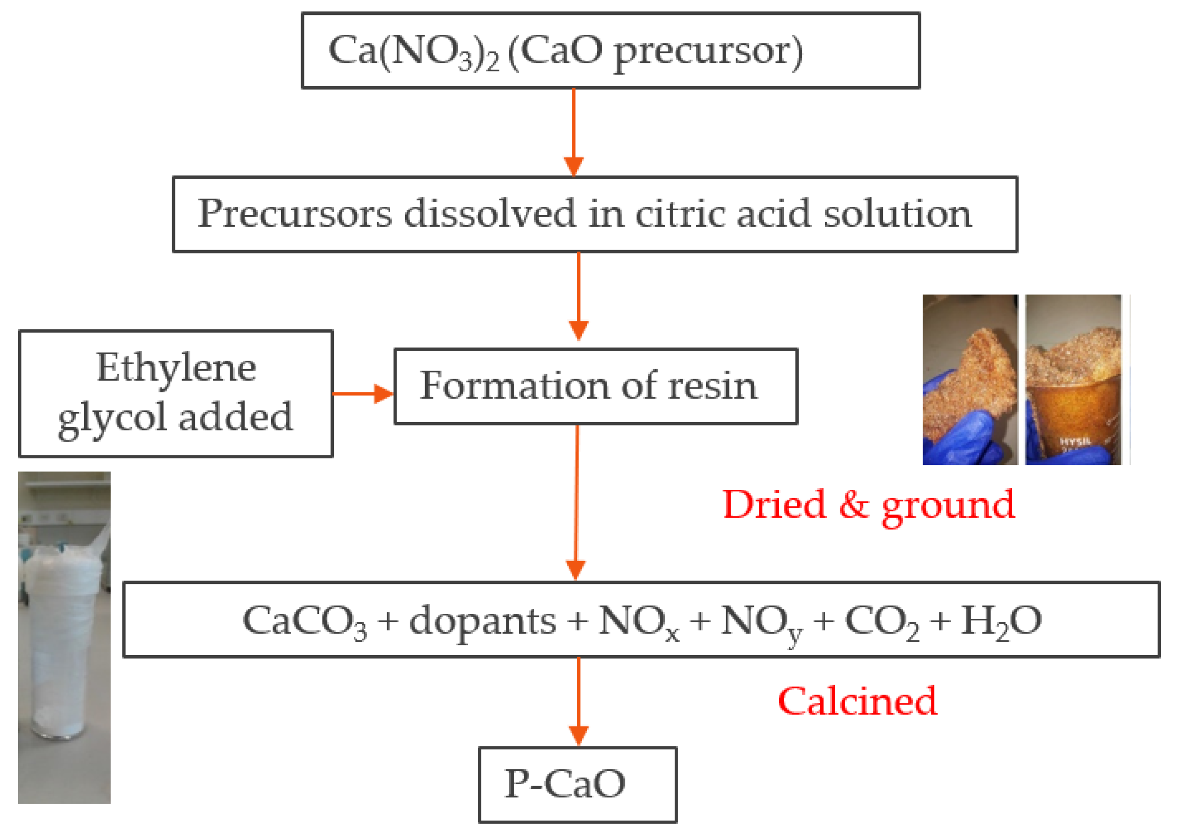
Pechini-synthesized CaO (denoted as P-CaO or P-CaCO₃ in its carbonate form) was prepared following the steps described by Jana, de la Peña O’Shea [45], which is also detailed in the experimental procedure of Fedunik-Hofman et al. [24]. First, 48 g of citric acid (CA; C₆H₈O₇; Sigma-Aldrich, 99.5% purity; 0.25 mol) was added to 100 mL of distilled water (Milli-Q >18.2 MΩ cm). The mixture was stirred at 70 °C until totally dissolved. Then, 11.8 g of the metal precursor Ca(NO₃)₂ (Sigma-Aldrich; 99.0% purity; 0.05 mol) was then added to the solution with a precursor to CA molar ratio of 1:5. The solution was stirred for 3 hours before the temperature was increased to 90 °C. Next, 9.23 mL of ethylene glycol (EG; HOCH₂CH₂OH; Sigma-Aldrich; 99.8% purity; 0.033 mol) was added with a molar ratio of CA to EG of 3:2. The resulting solution was further stirred at the same temperature to remove the excess solvent until the solution became a viscous resin. This resin was subsequently dried in an oven at 180 °C for 5 hours. The sample was then ground with an agate mortar and pestle to achieve fine particles and then calcined in a tube furnace. The furnace was programmed to heat from ambient temperature to 400 °C (10 °C min⁻¹ heating rate), where it was held for 2 hours, before heating to 900 °C and held for 4 hours. After calcination, the sample was ground again to ensure very fine particles were obtained. The experimental procedure is described in the schematic in Figure 1.

2.2. Cycling Analysis

The extent of conversion with cycling was monitored by thermogravimetric analysis (TGA) using a SETSYS Evolution 1750 TGA-DSC from Setaram. Two different experimental conditions were performed in order to carry out the different kinetic analysis methods.

To carry out a kinetic analysis using the Coats–Redfern method, non-isothermal calcination and carbonation was performed under two atmospheric conditions: Calcination under inert atmosphere (100% N₂; maximum temperature 850 °C) followed by carbonation under a mixed atmosphere (25% v/v CO₂); and calcination and carbonation under 100% CO₂ (maximum temperature 1000 °C). A total gas flow of 20 mL min⁻¹ was used for both conditions. Experimental conditions are detailed in

Table 1. Experimental conditions for kinetic analyses.

	Calcination			Carbonation
Experiment	Temp. (°C)	Atmosphere	Isotherm (min)	Temp. (°C)	Atmosphere	Isotherm (min)
Non-isothermal (mixed N2/CO2)	850	N2	0	–	75 v/v% N2 25 v/v% CO2	0
Non-isothermal (100% CO2)	1000	CO2	0	–	CO2	0
Isothermal	650/700/750	N2	20	650/700/750	75 v/v% N2 25 v/v% CO2	40

. For each experiment, ~18 mg of P-CaO (powder sample) was placed into a 100 μL alumina crucible and subjected to a temperature ramp from ambient to the maximum temperature, followed by subsequent cooling to ambient temperature. The experiment was repeated for four different heating rates (2.5, 5, 10, and 15 °C min⁻¹).

To implement generalized methods of kinetic analysis (i.e., intrinsic chemical reaction rate model and apparent model), it was necessary to carry out carbonation under isothermal conditions. For this case, P-CaO was heated to the set temperature (see Table 1) under 100% N₂ and held isothermally for 20 minutes. After this time, the gaseous atmosphere was adjusted to introduce 25% v/v CO₂ and held isothermally for 40 minutes to allow for carbonation. The sample was then cooled to ambient temperature. The heating and cooling rates were 10 °C min⁻¹ and a constant gas flow of 20 mL min⁻¹ was maintained.

For all experiments, a blank was performed under the same conditions and subtracted from each experiment to correct weight signal drifts. For the decomposition reaction of P-CaCO₃ to P-CaO, the extent of reaction, α, was determined using the fractional weight loss:

$$\alpha =\frac{m_i-m\left(t\right)}{m_i-m_f}$$

(2)

where m_i is the initial mass of the sample in grams, m(t) is the mass of the sample in grams after t minutes and m_f is the final mass of the sample in grams (after calcination). The carbonation conversion of P-CaO to P-CaCO₃ was calculated as follows:

$$X\left(t\right)=\left(\frac{m\left(t\right)-m_i}{m_{X=1}}\right)\times \left(\frac{M_{CaC{O}_3}}{M_{CaC{O}_3}-M_{CaO}}\right)$$

(3)

where m(t) is the mass of the sample in grams after t minutes under the carbonation atmosphere, m_i is the initial mass of the sample in grams (before carbonation), m_{X = 1} is the theoretical mass of the sample in grams after 100% carbonation conversion (43.97% mass gain), and M is the molar mass in g mol⁻¹.

This expression differs slightly from the means of calculating carbonation conversion usually utilized in literature [46]. The rationale is that prior to calcination in the thermogravimetric analyzer, P-CaO may still include CaCO₃ phases due to incomplete calcination in the furnace and adsorption of atmospheric CO₂. As a result, m(t) must be measured with reference to the theoretical mass after 100% carbonation conversion (which would occur during the first temperature ramp), as opposed to the initial mass of P-CaO.

3. Kinetic Analysis Methodology

Methods for solid–gas reactions are either differential, based on the differential form of the reaction model, f(α), or integral, based on the integral form g(α) [47].The expression for g(α) is the general expression of the integral form:

$$g\left(\alpha \right)={{\displaystyle \int }}_0^{\alpha }\frac{d\alpha }{f\left(\alpha \right)}=A{{\displaystyle \int }}_0^{t}exp\left(\frac{-E_a}{RT}\right)h\left(P\right)dt$$

(4)

where A is the pre-exponential factor (min⁻¹), R is the universal gas constant (kJ mol⁻¹ K⁻¹), T is the temperature (K), and h(P) is the pressure dependence term (dimensionless). Non-isothermal experiments employ a heating rate (β in K min⁻¹) which is constant with time, leading to Equations (5) and (6) [48].

$$\frac{d\alpha }{dT}=\frac{A}{\beta }exp\left(\frac{-E_a}{RT}\right)h\left(P\right)f\left(\alpha \right)$$

(5)

$$g\left(\alpha \right)=\frac{A}{\beta }{{\displaystyle \int }}_0^{T}exp\left(\frac{-E_a}{RT}\right)h\left(P\right)dT$$

(6)

Equation (5) is the starting point for differential methods of kinetic analysis, such as the Friedman (isoconversional) method. This method calculates E_a independently of a reaction model and requires multiple data sets [49]. It is referred to as a model-free technique as it avoids assumptions about a reaction mechanism and can identify multi-step reactions. This method is explained in detailed elsewhere [24,30].

Equation (6) is the starting equation for many integral methods of evaluating non-isothermal kinetic parameters with constant β. One example is the Coats–Redfern integral approximation method, referred to as a model-fitting method of kinetic analysis.

Model-fitting methods aim to determine the kinetic parameters of the reaction model integral by fitting obtained data to various known solid-state kinetic models and generally omit the pressure dependence term h(P) [47]. Kinetic models for reaction mechanisms can be categorized using different algebraic functions for f(α) and g(α), which can be found in Fedunik-Hofman et al. [30]. The general principle of model-fitting methods is to minimize the difference between the experimentally measured and calculated data for the given reaction rate expression [47].

3.1. Coats–Redfern Integral Approximation Method

Integral approximation methods replace the integral in Equation (6) with an integral approximation function, Q(x), where x is equal to E_a/RT. The integral can therefore be expressed by the following expression (complete derivations can be obtained in previously published works [30]):

$$g\left(\alpha \right)=\frac{AR}{E_a\beta }{T}^{2}exp\left(\frac{-E_a}{RT}\right)Q\left(x\right)$$

(7)

Many approximations for Q(x) exist and the Coats–Redfern approach is a commonly-used example:

$$Q\left(x\right)=\frac{\left(x-2\right)}{x}$$

(8)

Q(x) changes slowly with values of x and is close to unity [47]. Plots of $\ln \left[g\left(\alpha \right)/T^2\right]$ versus 1/T (Arrhenius plots) will result in a straight line for which the slope and intercept are E_a and A [50]:

$$ln\left[\frac{g\left(\alpha \right)}{T^2}\right]=-\left(\frac{E_a}{R}\right)\left(\frac{1}{T}\right)+ln\left[\frac{AR}{E_a\beta }\right]\left(1-\frac{2R{T}_{av}}{E_a}\right)$$

(9)

where T_av is the average temperature over the course of the reaction [51].

In order to find the kinetic parameters, Arrhenius plots for each g(α) mechanism can be produced. One pair of E_a and A for each mechanism can be obtained by linear data-fitting and the mechanism is chosen from the data fit with the best linear correlation coefficient (R²) [47].

Coats–Redfern cannot be applied to simultaneous multi-step reactions, although it can adequately represent a multi-step process with a single rate-limiting step [47]. For reactions with consecutive steps, the reaction can be split into multiple steps and model-fitting can be carried out for each step [47].

3.2. Master Plots

Master plots are characteristic curves independent of the condition of measurement which are obtained from experimental data [52]. In this paper, master plots were used to validate the reaction mechanism suggested by the Coats–Redfern method. One type of master plot is the Z(α) method, which is derived from a combination of the differential and integral forms of the reaction mechanism. Z(α) is defined as follows:

$$Z\left(\alpha \right)=f\left(\alpha \right)g\left(\alpha \right)$$

(10)

An alternative integral approximation for g(α) to the Coats–Redfern approximation in Equation (9) is $\frac{\pi \left(x\right)}{x},$ where $\pi$(x) is a polynomial function of x, for which several approximations exist [53,54]; i.e.:

$$\pi \left(x\right)=\frac{x^3+18x^2+88x+96}{x^4+20x^3+120x^2+240x+120}$$

(11)

Experimental values of Z(α) can be obtained with the following equation, which is derived in previously published works [30]:

$$Z\left(\alpha \right)=\frac{d\alpha }{dt}{T}^2\left[\frac{\pi \left(x\right)}{\beta T}\right]$$

(12)

For each of the reaction mechanisms, theoretical master plot curves can be plotted with Equation (10) (using the approximate algebraic functions f(α) described elsewhere [30]) and experimental values with Equation (12). The experimental values will provide a good fit for the theoretical curve with the same mechanism. As the experimental points have not been transformed into functions of the kinetic models, no prior assumptions are made for the kinetic mechanism [30].

3.3. Compensation Effect

Isoconversional methods, such as the Friedman method, do not explicitly suggest a reaction model. However, if the reaction model can be reasonably approximated with single-step reaction kinetics (if E_a does not vary significantly with α), the reaction mechanism can be determined using the compensation effect, which is described in detail elsewhere [24,30]. In this method, the isoconversional analysis of CaCO₃ calcination in Fedunik-Hofman et al. [24] is used to determine the average kinetic parameters (E_o and A_o), which are used to reconstruct the reaction model; i.e.:

$$g\left(\alpha \right)=\frac{A_0}{\beta }{{\displaystyle \int }}_0^{T_{\alpha }}exp\left(\frac{-E_0}{RT}\right)dT$$

(13)

Equation (13) is then plotted against the theoretical reaction models (see Section 3.1). In this way, experimental and theoretical curves can be compared to suggest a reaction mechanism.

3.4. Generalized Models for Kinetic Analysis of CaO Carbonation

In CaL, the calcination reaction commonly follows a thermal decomposition process that can be approximated by model-fitting and model-free methods. However, the carbonation reaction is more complex and is believed to be controlled by several mechanisms such as nucleation and growth, impeded CO₂ diffusion, or geometrical constraints related to the shape of the particles and pore size distribution of the powder [26]. Therefore, instead of using a purely kinetics-based approach for analysis of carbonation, functional forms of f(α) have been proposed to reflect these diverse mechanisms. This approach is referred to by Pijolat et al. as a generalized approach [55] and leads to a rate equation with both thermodynamic variables (e.g., temperature and partial pressures) and morphological variables [55].

Numerous studies suggest that the carbonation reaction takes place in two stages: An initial rapid conversion (kinetic control region) followed by a slower plateau (diffusion control region) [29]. These stages are generally analyzed separately using different models, and this approach is taken to perform a kinetic analysis for the carbonation reaction. Interested readers are directed to a previously published review paper for an extended discussion of generalized methods [30].

3.4.1. Chemical Reaction Control Region: Intrinsic Reaction Rate Model

The kinetic control region of the carbonation reaction is generally considered to be limited by heterogeneous surface chemical reaction kinetics, with the driving force for the reaction being the difference between bulk CO₂ pressure and equilibrium CO₂ pressure [56]. This region is typically described by the kinetic reaction rate constant k_s (m⁴ mol⁻¹ s⁻¹), which is considered to be an intrinsic property of the material [7].

In this paper, the carbonation of P-CaO is modeled using the grain model used by Sun et al. to determine the intrinsic rate constants of the CaO–CO₂ reaction [56]. Under kinetic control, the reaction rate, R (min⁻¹), is described by:

$$R=\frac{dX}{dt{\left(1-X\left(t\right)\right)}^{2/3}}=3r$$

(14)

where r is the grain model reaction rate (min⁻¹), which is assumed to be constant over the kinetic control region. In integral form the reaction rate can be expressed as:

$$\left[1-{\left(1-X\left(t\right)\right)}^{1/3}\right]=r\times t$$

(15)

Plotting $1–{\left(1–X\left(t\right)\right)}^{\raisebox{1ex}{$1$}\!\left/ \!\raisebox{-1ex}{$3$}\right.}$ versus t will produce a straight line plot due to the constant reaction rate. Values of r can be determined for each isothermal experiment and are taken to represent the true reaction rate at the zero conversion point [56], i.e.:

$$r_0=r$$

(16)

The specific reaction rate can also be expressed in power law form as:

$$R=3r{\left(1-X\left(t\right)\right)}^{-1/3}=56k_s{\left(P_{C{O}_2}-P_{C{O}_{2,eq}}\right)}^{n}S$$

(17)

where k_s is the intrinsic chemical reaction rate constant (mol m⁻² s⁻¹ kPa⁻ⁿ), $P_{C{O}_2}-P_{C{O}_{2,eq}}$ is the difference between the equilibrium and partial pressure of CO₂, n is the reaction order, and S is the specific surface area (m² g⁻¹). Sun et al. determined that at CO₂ partial pressures greater than 10 kPa, the reaction order n is zero-order [56]. At time 0, the following relationships are therefore established:

$$k_s=k_{0}exp\left(\frac{-E_a}{RT}\right)$$

(18)

where k₀ is the pre-exponential factor (mol. m² s⁻¹). An Arrhenius plot of slope lnr₀ vs 1/T can therefore be produced to determine the kinetic parameters E_a and k₀:

$$l{n}_{r_0}=ln\left(\frac{56k_0{S}_0}{3}\right)-\frac{E_a}{RT}$$

(19)

The intrinsic chemical reaction rate constant k_s (calculated using Equation (18)) can be converted to the rate constant k (min⁻¹) by means of:

$$k=k_{s}S{M}_{CaO}$$

(20)

3.4.2. Diffusion Control Region: Apparent Model

Following the kinetic control region, the reaction slows and becomes diffusion-limited [40]. A simplified generalized model (referred to as an apparent model) has been developed for the carbonation of CaO by Lee [37]. This model does not involve the use of morphological parameters and is described by the following equations:

$$X\left(t\right)=X_u\left[1-exp\left(-\frac{k}{X_u}t\right)\right]$$

(21)

$$X\left(t\right)=\frac{X_{u}t}{\left(X_u/k\right)+t}$$

(22)

where X_u is the ultimate conversion of CaO to CaCO₃ and k is the reaction rate (min⁻¹). A constant b is introduced to represent the time taken to attain half the ultimate conversion: X = X_u/2 at t = b. X_u can then be expressed as:

$$X_u=kb$$

(23)

Substituting Equation (23) into Equation (22) leads to:

$$X\left(t\right)=\frac{kbt}{b+t}$$

(24)

To determine the constants k and b using the least squares method, the equation is written in linear form:

$$\frac{1}{X\left(t\right)}=\frac{1}{k}\left(\frac{1}{t}\right)+\frac{1}{kb}$$

(25)

An Arrhenius plot can then be produced using the following relationship [57]:

$$ln\left(k\right)=-\frac{E_a}{R}\left(\frac{1}{T}\right)+lnA$$

(26)

The kinetic parameters E_a (kJ mol⁻¹) and A (min⁻¹) can therefore be obtained, as well as the diffusion rate constant k (min⁻¹).

4. Results of Kinetic Modeling

4.1. Calcination Kinetics Comparative Analysis

Calcination kinetics were modeled using Coats–Redfern, master plots, and isoconversional methods with compensation effects for two different atmospheres, as explained previously (see Section 3.1). The Coats–Redfern analysis under 100% N₂ will be discussed first. Figure 2a displays the Coats–Redfern Arrhenius plots for all of the theoretical reaction models (see Section 3.1), while Figure 2b shows selected reaction models with the highest correlation coefficients, which are also presented in

Table 2. Kinetic parameters for calcination obtained from P-CaCO₃ (100% N₂ atmosphere) (average over four heating rates) compared with literature results (CaCO₃ decomposition under inert atmosphere).

Kinetic Model	Ea (kJ mol−1)	A (min−1)	Correlation Coefficient (R2)	Material and Reference
A2	108.73	3.5 × 104	0.9924	P-CaCO3 This work
A3	67.11	1.7 × 102	0.9913	This work
A4	46.30	1.1 × 101	0.9900	This work
R2	203.57	2.1 × 109	0.9995	This work
R3	213.12	5.0 × 109	0.9982	This work
F1	233.59	2.3 × 1011	0.9933	This work
D1	371.14	1.0 × 1018	0.9985	This work
R2	180.12	1.2 × 107	-	CaCO3 [50]
F1	190.46	3.4 × 107	-	CaCO3 [58]
R3	187.1	-	-	CaCO3 [54]
D1	224.21	3.0 ×· 104	-	CaCO3 [59]

The kinetic models are classified as follows. A2–4 are the Avrami–Erofeyev nucleation models, where 2–4 refer to the exponential in the algebraic function. R2–3 are the geometric contraction models, where R2 uses a contracting area model and R3 uses a contracting volume model. F1 refers to a first-order reaction model and D1 to a first-order diffusion model.

.

Correlation coefficients are seen to be very high for all reaction mechanisms, while calculated activation energies vary between 47 and 370 kJ mol⁻¹. By a small margin, the highest correlation coefficient is produced by the R2 geometric model, which determined an E_a of 204 kJ mol⁻¹. These kinetic parameters are typical for the calcination of CaCO₃ under an inert atmosphere. Literature results generally produce values of E_a between 180 and 224 kJ mol⁻¹ [30], showing a lack of consensus on the calcination reaction model (see Table 2). Physical descriptions of the reaction models referenced in Table 2 are provided in a review of kinetics applied to CaL [30].

As for the experiment under N₂, Coats–Redfern Arrhenius plots (Figure 3) and kinetic parameters for selected reaction models (

Table 3. Kinetic parameters for calcination obtained from P-CaO material (100% CO₂ atmosphere; average over four heating rates) compared with literature results.

Kinetic Model	Ea (kJ mol−1)	A (min−1)	Correlation Coefficient (R2)	Material and Reference
A2	599.6	3.4 × 1027	0.9788	P-CaCO3 This work
A3	419.9	4.5 × 1019	0.9781	This work
A4	309.9	6.2 × 1014	0.9774	This work
F1	1219.2	2.9 × 1054	0.9795	This work
R3	1037.6	3.9 × 1040	-	CaCO3 [60]
2nd order	2104.6	1090	-	CaCO3 [31]

) are presented for an experiment under 100% CO₂. Under this atmosphere, calculated activation energies are much higher, ranging from 300 to 600 kJ mol⁻¹ when modeled by the nucleation models to 1200 kJ mol⁻¹ when fitted with a first-order model. This is due to the high gradients in the Arrhenius plots under 100% CO₂, which mathematically leads to high activation energies. High values of E_a are also obtained in the few literature studies carried out under 100% CO₂ [31,60]. Caldwell et al. attribute this to the fact that the temperature range of decomposition becomes higher and narrower as the percentage of CO₂ increases, resulting in a higher apparent activation energy [31].

Examining the correlation coefficients suggests that the reaction mechanism of P-CaCO₃ decomposition under CO₂ can be modeled by a first-order reaction or Avrami nucleation A2 and A3 (see Table 3). Correlation coefficients are seen to be lower than the models under N₂ (see Table 2). As for the inert atmosphere, there is no consensus on the reaction model in published literature.

Intraparticle and transport resistances may affect reaction rates and reaction mechanisms and have been suggested as the cause of large values of E_a for CaCO₃ calcination [60]. In a decomposition mechanism where the reaction advances inwards from the outside of the particle, smaller particles will decompose more quickly [30,61]. If particle sizes are too large, it has been suggested that the reaction may become limited by mass transport, as opposed to the chemical reaction. However, the influence of particle sizes has been found to be small at high CO₂ partial pressures [33], so intraparticle mass transport effects on the kinetic parameters can be ruled out as the cause of the overestimated kinetic parameters for the experiments under 100% CO₂. [7].

From the comparison of experiments under different atmospheres, it is evident that calculated activation energies can be highly variable. Although there is believed to be a single, intrinsic activation energy for the calcination reaction, values determined experimentally with model-fitting methods have been described as “effective” activation energies [48]. For the experiment under 100% CO₂, in particular, the large disparity in activation energies determined by different reaction models (310–1220 kJ mol⁻¹) and the lower correlation coefficients suggest that model-fitting methods may be unsuitable for calcination under 100% CO₂. An alternative is the use of model-free methods to determine kinetic parameters, as in the previous study of Fedunik-Hofman et al., which used the isoconversional Friedman method to obtain kinetic parameters which vary over the course of the reaction [24].

For both experimental atmospheres, rate constants could not be evaluated using model-fitting methods, as the Coats–Redfern method produced unreasonably large values of k(T). This is because both k(T) and f(α) vary simultaneously under non-isothermal conditions. This causes the Arrhenius parameters for non-isothermal experiments to be highly variable and exhibit a strong dependence on the reaction model (see Table 3) [62]. It has been established that the rate constant cannot be viably predicted by model-fitting methods due to the ambiguity of the kinetic triplet [62]. As suggested previously, isoconversional methods are an alternative means of determining rate constants [24].

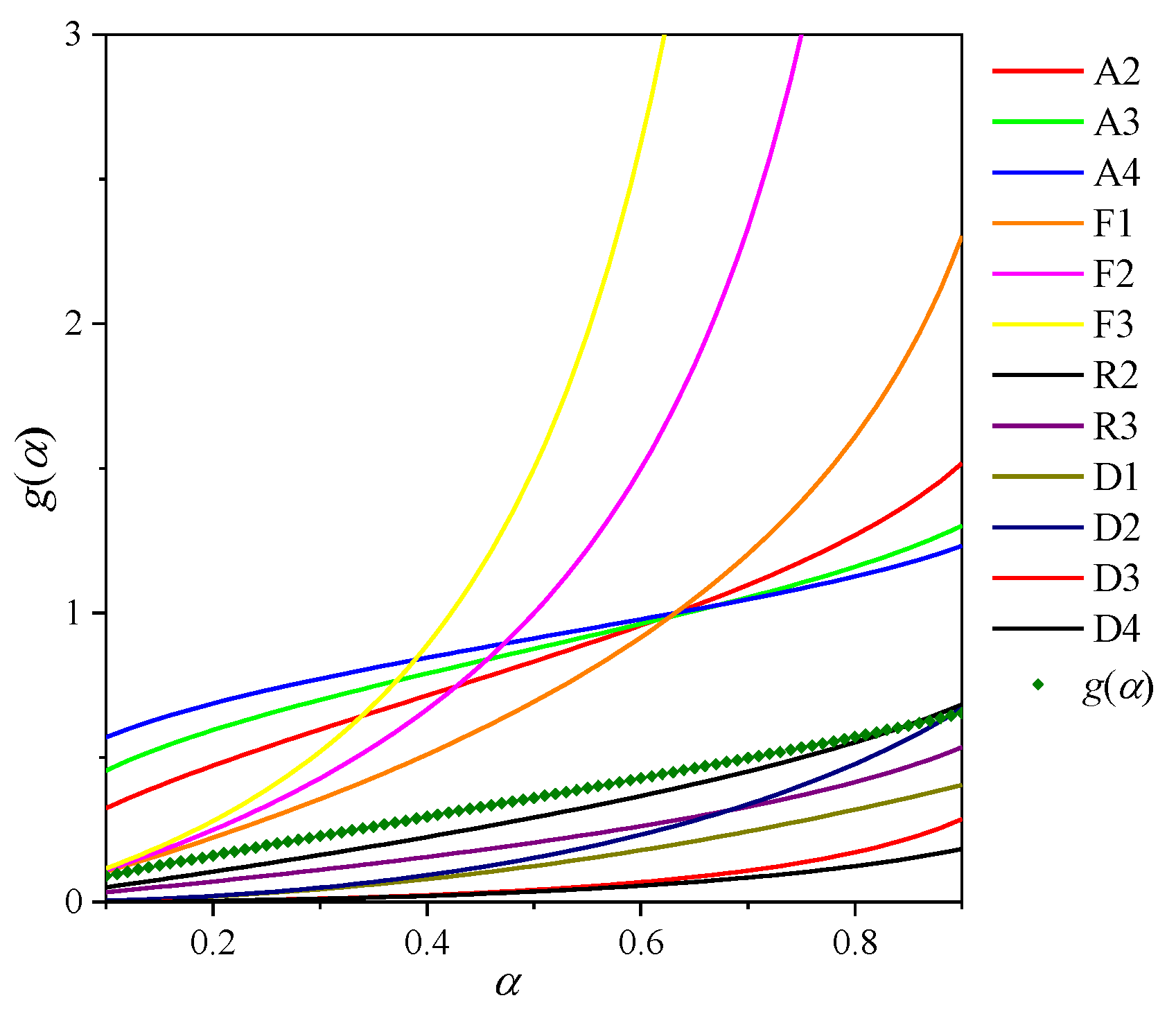
As a means of comparison and to aid in a selection of a reaction mechanism, a master plot was produced using the experimental data (non-isothermal experiments carried out under both experimental atmospheres).

Examining the Z(α) master plot in Figure 4a for calcination under N₂, there is good correlation between the experimental data points and the R3 geometric model, which is most pronounced for the experiments performed at 10 and 15 K min⁻¹. The lower heating rates experiments show a poorer fit, which could be the result of heat transfer effects. This result correlates with the mechanism suggested by the Coats–Redfern method, which produces high correlation coefficients for both geometric models R2 and R3, as well as literature results (see Table 2).

For calcination under CO₂ (Figure 4b), a good correlation exists for the experimental data points and the Avrami curves A2 and A3, as well as the first-order chemical reaction model F1. Different experimental heating rates are seen to suggest different mechanisms. For example, the 2.5 K min⁻¹ heating rate suggests the mechanism is A3, while 5 K min⁻¹ suggests A2 and 10 K min⁻¹ suggests F1. It is important to note that F1 is a special case of Avrami nucleation [63], as can be seen by the identical shape of the curves, which only differ in magnitude due to the different coefficient n in g(α). Differences in the magnitude of the curves for different heating rates could be the result of heat transfer effects. Therefore, it can be concluded that the calcination reaction under CO₂ is a nucleation process. The reaction mechanism suggested by the master plot generally reflects those in the literature carried out using generalized (non-model-fitting) methods, which are summarized elsewhere [30]. Studies typically suggest that the decomposition reaction can be modeled by either Avrami nucleation [26] or first-order chemical reaction F1 [32,58], which is logical when taking into account that F1 is a special case of nucleation.

As a further means of comparison, the model-fitting results presented previously were compared with published results which employed the isoconversional Friedman method, carried out by the authors using the same experimental data [24]. The results of the analysis are summarized in

Table 4. Kinetic parameters for calcination obtained from P-CaO material using the Friedman method [24].

Experimental Atmosphere	CO2	N2
Ea (kJ mol−1)	430–171	171–147
Eo (kJ mol−1)	307	164
Aα (min−1)	3.8 × 1034–2.9 × 105	1.5 × 107–3.7 × 104
Ao (min−1)	–	3.13· 106
Max k (min−1)	0.023	0.012

, which also presents average values of E_a over the course of the reaction (E_o). A detailed explanation of the assumption of single-step reaction kinetics is presented elsewhere [30]. The equilibrium pressure, P₀ (kPa), of the gaseous product is seen to have a significant influence on dα/dt and, hence, the activation energies under the 100% CO₂ atmosphere [24] (see Table 4).

The compensation effect was used as an alternative means of determining a reaction mechanism for calcination. This method was only applied for calcination under N₂, due to the large variation in kinetic parameters under CO₂ [24] (see Section 3.3). Figure 5 shows a comparison of the experimental and theoretical reaction models, which are compared to suggest a reaction mechanism. The plot shows that the best fitting reaction mechanism is the R2 (contracting area) geometric reaction model, which produces a correlation coefficient of 0.9919. This model also produced a high correlation coefficient in the Coats–Redfern analysis (R² > 0.999; see Table 2). The activation energy determined with Coats–Redfern is 30% higher than the average Friedman value (213 compared to 164 kJ mol⁻¹), although the values are still within the range obtained in the literature for CaCO₃ calcination [30]. In conclusion, the R2 model (contracting area) is the mechanism which most accurately models the calcination of CaCO₃ under pure N₂, in agreement with the literature [50], which has been verified using both Coats–Redfern and compensation effect methods.

It is important to note that the nucleation models and the R2 reaction model are proposed as the mechanisms most consistent with kinetic data for calcination of CaCO₃ under 100% CO₂ and N₂, respectively. As set out by Vyazovkin and Wight in their discussion of the solid state reactions and the extraction of Arrhenius parameters from thermal analysis, one of the fundamental tenets of chemical kinetics is that no reaction mechanism can ever be proved on the basis of kinetic data alone [64]. Despite not allowing for complete isolation of the experimental reaction without influence from physical processes (i.e., diffusion, adsorption, desorption), the suggested reaction models are useful for drawing reasonable mechanistic conclusions.

4.2. Carbonation Kinetics Comparative Analysis

In order to implement generalized kinetic models, isothermal experiments were carried out, as detailed in Section 2.2. The chemical reaction control region was modeled using an intrinsic reaction rate model, while the diffusion control region was modeled using an apparent model.

4.2.1. Chemical Reaction Control Region (Intrinsic Reaction Rate Model)

Using the methodology in Section 3.4.1, plots of the carbonation conversion were produced for three isothermal experiments (see Figure 6 and Figure 7). Specific reaction rates for each isothermal experiment are presented in

Table 5. Carbonation reaction: Intrinsic reaction rate model parameters.

T (°C)	ro (s−1 × 10−4)	R2	k0 (mol m−2 s−1 × 10−5)	k (min−1)
650	6.41	0.9950	2.88	0.137
700	7.33	0.9927	3.23	0.173
750	8.00	0.9999	3.59	0.213

. The kinetic parameters were obtained by performing data fitting on the Arrhenius plot (Figure 7b). The correlation coefficients produced by linear data fitting are high for all experimental temperatures (R² > 0.99; see Table 5), which confirms that the chemical reaction region is well-modeled by the intrinsic reaction rate model. An activation energy of 17.45 kJ mol⁻¹ was obtained for this region.

4.2.2. Diffusion Control Region (Apparent Model)

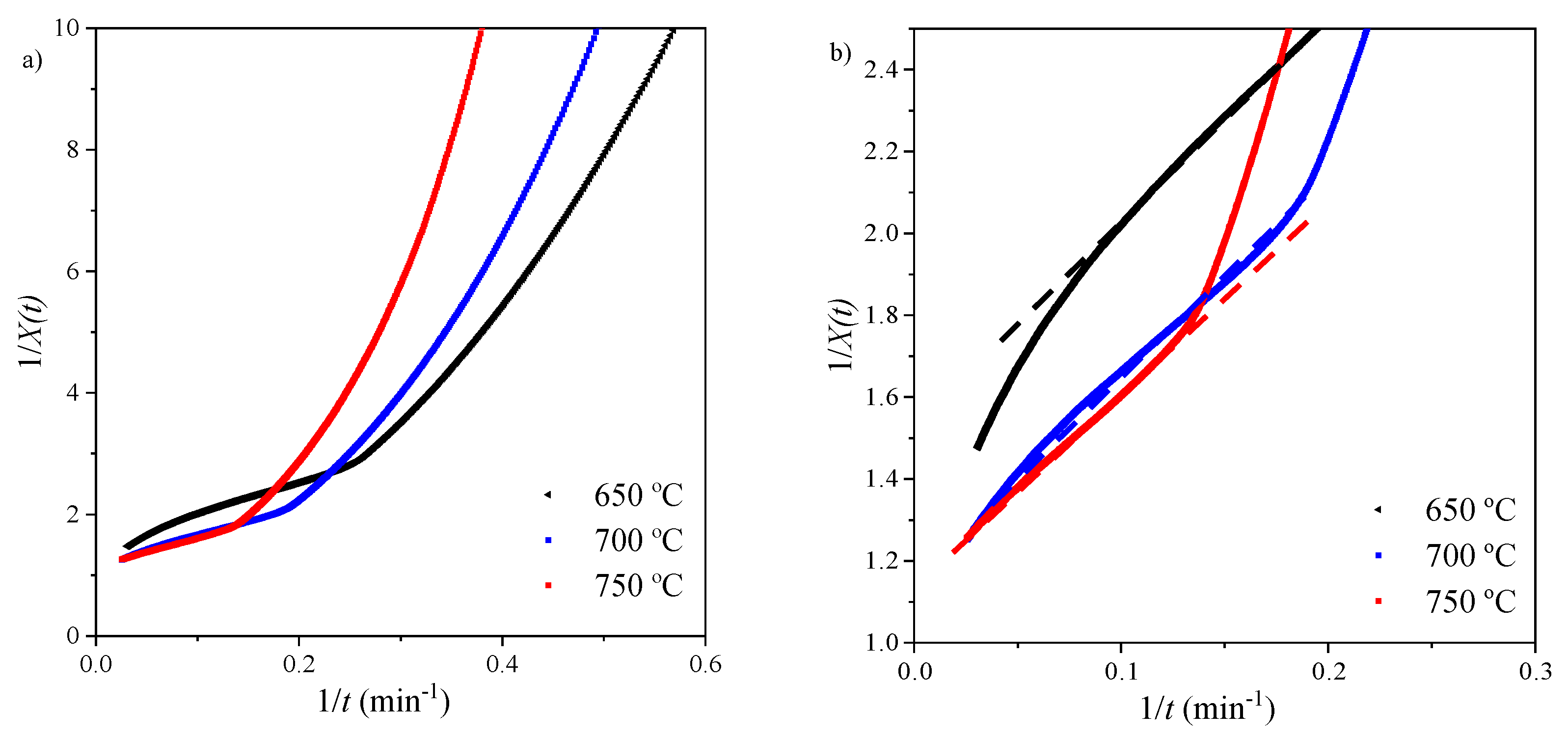
Using the methodology described in Section 3.4.2, an apparent model was used to determine the kinetic parameters of the diffusion control region. Data fitting plots are shown in Figure 8 and Figure 9 and apparent model parameters are recorded in

Table 6. Carbonation reaction: Apparent model parameters.

T (°C)	k (min−1)	b (min)	Xu
650	0.098	8.80	0.863
700	0.158	5.54	0.875
750	0.210	4.16	0.872

.

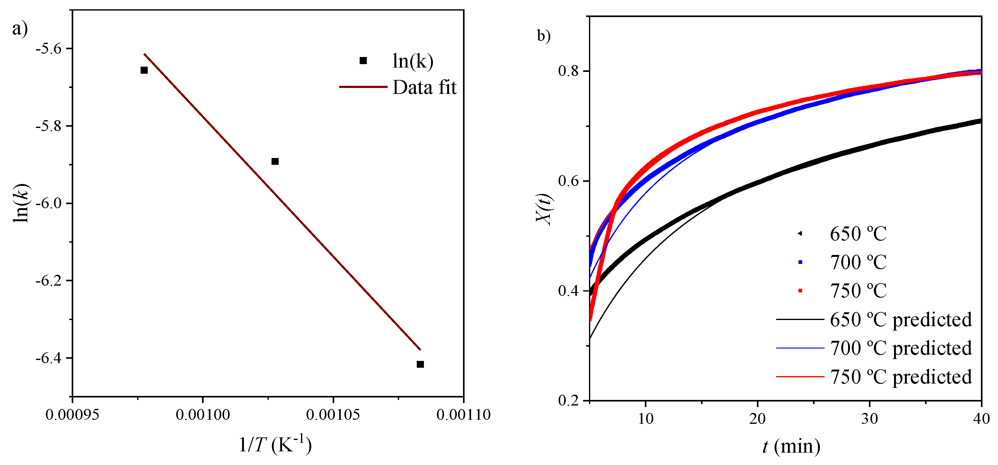
In order to validate the model, the obtained values of X_u and k were used to calculate X(t) (Equation (23)) and plotted against the isothermal data for the diffusion region. Figure 9b shows a good agreement between experimental data and the model. The kinetic parameters were obtained by performing data fitting on the Arrhenius plot (Figure 9a). An activation energy of 59.95 kJ mol⁻¹ was calculated for this region.

Kinetic parameters for both the kinetic and diffusion control regions are presented in

Table 7. Carbonation reaction: Kinetic parameters. k_s and D are averages over the temperature range 650, 700, and 750 °C. S is provided in as-synthesized state or after one cycle.

Kinetic Control Region
Reference	This Work	Sun et al. [56]	Lee [37] Data: Bhatia and Perlmutter [25]	Lee [37] Data: Gupta and Fan [39]	Grasa et al. [17]
Material	P-CaO	Strassburg limestone	Calcined limestone	Calcined precipitated CaCO3	Katowice limestone
Method	Intrinsic reaction rate model	Intrinsic reaction rate model	Apparent model	Apparent model	Pore model
T (°C)	k (min−1)
650	0.24	0.97	0.925 *	0.858	–
700	0.27	0.81	–	–	–
750	0.30	0.67	–	–	–
S (m2 g−1)	13.8	29	15.6	12.8	12.9 **
Ea (kJ mol−1)	17.45	24.0	72.2	72.7	19.2
ks (m4 kmol−1 s−1)	3.34 × 10−6	4.68 × 10−6	6.0 × 10−7	–	5.29 × 10−6
Diffusion control region
Method	Apparent model	–	Apparent model	Apparent model	Pore model
T (°C)	k (min−1)
650	0.098	–	0.344 *	0.357	–
700	0.158	–	–	–	–
750	0.210	–	–	–	–
Ea (kJ mol−1)	59.95	–	189.3	102.5	163
D (m2 s−1)	–	–	–	4.32 × 10−6	–

* Calculated at 655 °C [37]; ** calculated from specific surface area (m² m⁻³) assuming ρ (non-porous CaCO₃) of 2710 kg m⁻³.

and compared with selected literature results. Lee states that k can be regarded as the intrinsic chemical reaction rate constant k_s [37], as well as the diffusion constant D, although the different units mean that it cannot be directly compared with reaction rate constants for studies such as those using pore models [17].

For both the chemical reaction and diffusion control regions, the reaction rates and values of X_u (see Table 6) tend to increase with increasing temperature, which is consistent with reaction kinetics increasing with higher temperatures (as described by Arrhenius relationships; i.e., Equation (4)). The reaction rates for P-CaO are seen to be slightly slower than those in the literature. The activation energies of P-CaO are also slightly lower than expected for both the kinetic control region (literature values typically fall between 20 and 32 kJ mol⁻¹) and the diffusion region (literature values are typically between 80 and 200 kJ mol⁻¹ ) [30].

The variation in the activation energies has been attributed to the differences in morphology and texture of the CO₂ sorbent [46,56]. While it has been suggested that morphology of CaO does not greatly influence kinetics in the kinetic control region [28], outlying values have been attributed to diffusion limitations in the material [37]. Lee postulated that lower activation energies are associated with microporous materials that are susceptible to pore plugging, which would limit diffusion of CO₂, and is also associated with low carbonation conversion [37]. A study by Grasa et al. determined a much higher diffusion E_a of 163 kJ mol⁻¹ for mesoporous limestone [17], which has been associated with resistance to pore plugging [39]. In the case of P-CaO, however, BET analysis showed that the material was largely nonporous, with the majority of pore volume in the macroporous region [24]. Nevertheless, the lower diffusion activation energy could be the result of incomplete carbonation conversion (see Table 6).

Cycling experiments with P-CaO performed elsewhere [24] show good performance with cycling, which suggests that the reaction rates, although initially slower than other materials, will be retained with subsequent cycles. Future analysis could involve calculation of kinetic parameters after multiple isothermal cycles. Carrying out a kinetic analysis with another generalized method is also recommended, as the apparent method uses only a small number of data points to produce an Arrhenius equation.

5. Conclusions

This paper has presented a comparative kinetic analysis of the reactions for CaL, using both inert atmospheres/low CO₂ concentrations, as is typically performed in the literature, and the more rarely-used 100% CO₂ atmosphere. Additionally, it has discussed the validity of model-fitting methods in direct comparison with isoconversional and generalized methods, which has not been carried out previously. The experimental conditions, material properties, and the kinetic method have been found to strongly influence the kinetic parameters for both calcination and carbonation reactions. The main conclusions of the study are summarized as follows:

For the calcination of synthesized CaCO₃ under N₂, an E_a of 204 and 233.6 kJ mol⁻¹ was obtained by model-fitting using the R2 geometric model and F1 model, respectively, which is consistent with the literature results. Calcination of the same material determined an average E_a of 164 kJ mol⁻¹ using an isoconversional method. The compensation effect also suggested that the best reaction model was R2. For calcination under CO₂, much higher values of E_a were obtained, i.e., 310 kJ mol⁻¹ with A4 (Avrami nucleation) and 1220 kJ mol⁻¹ with the F1 model, while isoconversional results ranged between 170 and 530 kJ mol⁻¹, which was attributed to the major morphological changes in the material under CO₂ [24].

From this study, we can conclude that a multiple heating-rate isoconversional method, such as Friedman, should first be carried out to arrive at non-mechanistic parameters. It will also show whether the kinetic parameters vary over the course of the reaction. Then, if the activation energy does not vary significantly under the experimental atmosphere (as is the case for calcination of CaCO₃ under inert gas), the compensation effect can be used to suggest a reaction model. As a means of comparison, a model-fitting method such as Coats–Redfern can be applied over the whole reaction to determine kinetic parameters based on several reaction models. This can be corroborated with master plots. Where applicable, the reaction model with the highest correlation coefficient can be compared with the results of the isoconversional analysis. If the same kinetic parameters are obtained, greater confidence can be placed in the results of the analysis.

If the activation energy does vary significantly under the experimental atmosphere (as is the case for calcination of CaCO₃ under CO₂), the Coats–Redfern method is not recommended, as the discrete values of kinetic parameters will not capture the variation in reaction kinetics. Additionally, the compensation effect cannot be applied, as it requires single values of kinetic parameters. In this case, an isoconversional analysis is the best option for obtaining kinetic parameters.

The carbonation of synthesized CaO was modeled using an intrinsic chemical reaction rate model (for the kinetic control region) and apparent model (for the diffusion region), and subsequently compared with the literature. An activation energy of 17.45 kJ mol⁻¹ was obtained for the kinetic control region, and 59.95 kJ mol⁻¹ for the diffusion region. Lower values of E_a compared to the literature could be attributed to the incomplete carbonation conversion. For this synthesized material, the generalized models proved to model the two carbonation regions with high accuracy. For further studies, material characterization (i.e., scanning/transmission electron microscopy, physisorption characterization, and/or porosimetry) is recommended prior to selecting a generalized kinetic analysis method.

References

- Bayon, A.; Bader, R.; Jafarian, M.; Fedunik-Hofman, L.; Sun, Y.; Hinkley, J.; Miller, S.; Lipiński, W. Techno-economic assessment of solid–gas thermochemical energy storage systems for solar thermal power applications. Energy 2018, 149, 473–484. [Google Scholar] [CrossRef]
- Edwards, S.; Materić, V. Calcium looping in solar power generation plants. Sol. Energy 2012, 86, 2494–2503. [Google Scholar] [CrossRef]
- Angerer, M.; Becker, M.; Härzschel, S.; Kröper, K.; Gleis, S.; Vandersickel, A.; Spliethoff, H. Design of a MW-scale thermo-chemical energy storage reactor. Energy Rep. 2018, 4, 507–519. [Google Scholar] [CrossRef]
- Ströhle, J.; Junk, M.; Kremer, J.; Galloy, A.; Epple, B. Carbonate looping experiments in a 1 MWth pilot plant and model validation. Fuel 2014, 127, 13–22. [Google Scholar] [CrossRef]
- André, L.; Abanades, S.; Flamant, G. Screening of thermochemical systems based on solid-gas reversible reactions for high temperature solar thermal energy storage. Renew. Sustain. Energy Rev. 2016, 64, 703–715. [Google Scholar] [CrossRef]
- Stanmore, B.R.; Gilot, P. Review: Calcination and carbonation of limestone during thermal cycling for CO2 sequestration. Fuel Process. Technol. 2005, 86, 1707–1743. [Google Scholar] [CrossRef]
- Grasa, G.; Abanades, J.C.; Alonso, M.; González, B. Reactivity of highly cycled particles of CaO in a carbonation/calcination loop. Chem. Eng. J. 2008, 137, 5615–5667. [Google Scholar] [CrossRef]
- King, P.L.; Wheeler, V.M.; Renggli, C.J.; Palm, A.B.; Wilson, S.A.; Harrison, A.L.; Morgan, B.; Nekvasil, H.; Troitzsch, U.; Mernagh, T.; et al. Gas–Solid Reactions: Theory, Experiments and Case Studies Relevant to Earth and Planetary Processes. Rev. Mineral. Geochem. 2018, 84, 1–56. [Google Scholar] [CrossRef]
- Boot-Handford, M.E.; Abanades, J.C.; Anthony, E.J.; Blunt, M.J.; Brandani, S.; Mac Dowell, N.; Fernández, J.R.; Ferrari, M.-C.; Gross, R.; Hallett, J.P.; et al. Carbon capture and storage update. Energy Environ. Sci. 2014, 7, 130–189. [Google Scholar] [CrossRef]
- Hanak, D.P.; Manovic, V. Calcium looping with supercritical CO2 cycle for decarbonisation of coal-fired power plant. Energy 2016, 102, 343–353. [Google Scholar] [CrossRef]
- Shimizu, T.; Hirama, T.; Hosoda, H.; Kitano, K.; Inagaki, M.; Tejima, K. A Twin Fluid-Bed Reactor for Removal of CO2 from Combustion Processes. Chem. Eng. Res. Des. 1999, 77, 62–68. [Google Scholar] [CrossRef]
- Martínez, I.; Grasa, G.; Murillo, R.; Arias, B.; Abanades, J.C. Kinetics of Calcination of Partially Carbonated Particles in a Ca-Looping System for CO2 Capture. Energy Fuels 2012, 26, 1432–1440. [Google Scholar] [CrossRef]
- Diego, M.; Martinez, I.; Alonso, M.; Arias, B.; Abanades, J. Calcium looping reactor design for fluidized-bed systems. In Calcium and Chemical Looping Technology for Power Generation and Carbon Dioxide (CO2) Capture; Fennell, P., Anthony, B., Eds.; Woodhead Publishing: Cambridge, UK, 2015; pp. 107–138. [Google Scholar]
- Alonso, M.; Rodriguez, N.; Gonzalez, B.; Arias, B.; Abanades, J.C. Capture of CO2 during low temperature biomass combustion in a fluidized bed using CaO. Process description, experimental results and economics. Energy Procedia 2011, 4, 795–802. [Google Scholar] [CrossRef]
- Bouquet, E.; Leyssens, G.; Schönnenbeck, C.; Gilot, P. The decrease of carbonation efficiency of CaO along calcination–carbonation cycles: Experiments and modelling. Chem. Eng. Sci. 2009, 64, 2136–2146. [Google Scholar] [CrossRef]
- Sun, P.; Grace, J.R.; Lim, C.J.; Anthony, E.J. A discrete-pore-size-distribution-based gas-solid model and its application to the CaO + CO2 reaction. Chem. Eng. Sci. 2008, 63, 57–70. [Google Scholar] [CrossRef]
- Grasa, G.; Murillo, R.; Alonso, M.; Abanades, J.C. Application of the random pore model to the carbonation cyclic reaction. AIChE J. 2009, 55, 1246–1255. [Google Scholar] [CrossRef]
- Yue, L.; Lipiński, W. Thermal transport model of a sorbent particle undergoing calcination–carbonation cycling. AIChE J. 2015, 61, 2647–2656. [Google Scholar] [CrossRef]
- Yue, L.; Lipiński, W. A numerical model of transient thermal transport phenomena in a high-temperature solid–gas reacting system for CO2 capture applications. Int. J. Heat Mass Transf. 2015, 85, 1058–1068. [Google Scholar] [CrossRef]
- Lasheras, A.; Ströhle, J.; Galloy, A.; Epple, B. Carbonate looping process simulation using a 1D fluidized bed model for the carbonator. Int. J. Greenh. Gas Control 2011, 5, 686–693. [Google Scholar] [CrossRef]
- Romano, M. Coal-fired power plant with calcium oxide carbonation for postcombustion CO2 capture. Energy Procedia 2009, 1, 1099–1106. [Google Scholar] [CrossRef]
- Martínez, I.; Murillo, R.; Grasa, G.; Abanades, J.C. Integration of a Ca-looping system for CO2 capture in an existing power plant. Energy Procedia 2011, 4, 1699–1706. [Google Scholar] [CrossRef]
- Sarrión, B.; Perejón, A.; Sánchez-Jiménez, P.E.; Pérez-Maqueda, L.A.; Valverde, J.M. Role of calcium looping conditions on the performance of natural and synthetic Ca-based materials for energy storage. J. CO2 Util. 2018, 28, 374–384. [Google Scholar] [CrossRef]
- Fedunik-Hofman, L.; Bayon, A.; Hinkley, J.; Lipiński, W.; Donne, S.W. Friedman method kinetic analysis of CaO-based sorbent for high-temperature thermochemical energy storage. Chem. Eng. Sci. 2019, 200, 236–247. [Google Scholar] [CrossRef]
- Bhatia, S.K.; Perlmutter, D.D. Effect of the product layer on the kinetics of the CO2-lime reaction. AIChE J. 1983, 29, 79–86. [Google Scholar] [CrossRef]
- Valverde, J.M.; Sanchez-Jimenez, P.E.; Perez-Maqueda, L.A. Limestone calcination nearby equilibrium: Kinetics, CaO crystal structure, sintering and reactivity. J. Phys. Chem. C 2015, 119, 1623–1641. [Google Scholar] [CrossRef]
- Ingraham, T.R.; Marier, P. Kinetic studies on the thermal decomposition of calcium carbonate. Can. J. Chem. Eng. 1963, 41, 170–173. [Google Scholar] [CrossRef]
- Salaudeen, S.A.; Acharya, B.; Dutta, A. CaO-based CO2 sorbents: A review on screening, enhancement, cyclic stability, regeneration and kinetics modelling. J. CO2 Util. 2018, 23, 179–199. [Google Scholar] [CrossRef]
- Kierzkowska, A.M.; Pacciani, R.; Müller, C.R. CaO-based CO2 sorbents: From fundamentals to the development of new, highly effective materials. ChemSusChem 2013, 6, 1130–1148. [Google Scholar] [CrossRef]
- Fedunik-Hofman, L.; Bayon, A.; Donne, S.W. Kinetics of Solid-Gas Reactions and Their Application to Carbonate Looping Systems. Energies 2019, 12, 2981. [Google Scholar] [CrossRef]
- Caldwell, K.M.; Gallagher, P.K.; Johnson, D.W. Effect of thermal transport mechanisms on the thermal decomposition of CaCO3. Thermochim. Acta 1977, 18, 15–19. [Google Scholar] [CrossRef]
- Rodriguez-Navarro, C.; Ruiz-Agudo, E.; Luque, A.; Rodriguez-Navarro, A.B.; Ortega-Huertas, M. Thermal decomposition of calcite: Mechanisms of formation and textural evolution of CaO nanocrystals. Am. Mineral. 2009, 94, 578–593. [Google Scholar] [CrossRef]
- Khinast, J.; Krammer, G.F.; Brunner, C.; Staudinger, G. Decomposition of limestone: The influence of CO2 and particle size on the reaction rate. Chem. Eng. Sci. 1996, 51, 623–634. [Google Scholar] [CrossRef]
- Dai, P.; González, B.; Dennis, J.S. Using an experimentally-determined model of the evolution of pore structure for the calcination of cycled limestones. Chem. Eng. J. 2016, 304, 175–185. [Google Scholar] [CrossRef]
- García-Labiano, F.; Abad, A.; de Diego, L.F.; Gayán, P.; Adánez, J. Calcination of calcium-based sorbents at pressure in a broad range of CO2 concentrations. Chem. Eng. Sci. 2002, 57, 2381–2393. [Google Scholar] [CrossRef]
- Li, Z.; Sun, H.; Cai, N. Rate equation theory for the carbonation reaction of CaO with CO2. Energy Fuels 2012, 26, 4607–4616. [Google Scholar] [CrossRef]
- Lee, D.K. An apparent kinetic model for the carbonation of calcium oxide by carbon dioxide. Chem. Eng. J. 2004, 100, 71–77. [Google Scholar] [CrossRef]
- Nouri, S.M.M.; Ebrahim, H.A. Kinetic study of CO2 reaction with CaO by a modified random pore model. Pol. J. Chem. Technol. 2016, 18, 93–98. [Google Scholar] [CrossRef]
- Gupta, H.; Fan, L.-S. Carbonation−Calcination Cycle Using High Reactivity Calcium Oxide for Carbon Dioxide Separation from Flue Gas. Ind. Eng. Chem. Res. 2002, 41, 4035–4042. [Google Scholar] [CrossRef]
- Mess, D.; Sarofim, A.F.; Longwell, J.P. Product layer diffusion during the reaction of calcium oxide with carbon dioxide. Energy Fuels 1999, 13, 999–1005. [Google Scholar] [CrossRef]
- Bouineau, V.; Pijolat, M.; Soustelle, M. Characterisation of the chemical reactivity of a CaCO3 powder for its decomposition. J. Eur. Ceram. Soc. 1998, 18, 1319–1324. [Google Scholar] [CrossRef]
- Manovic, V.; Charland, J.-P.; Blamey, J.; Fennell, P.S.; Lu, D.Y.; Anthony, E.J. Influence of calcination conditions on carrying capacity of CaO-based sorbent in CO2 looping cycles. Fuel 2009, 88, 1893–1900. [Google Scholar] [CrossRef]
- Valverde, J.M.; Sanchez-Jimenez, P.E.; Perez-Maqueda, L.A. Calcium-looping for post-combustion CO2 capture. On the adverse effect of sorbent regeneration under CO2. Appl. Energy 2014, 126, 161–171. [Google Scholar] [CrossRef]
- Symonds, R.T.; Lu, D.Y.; Manovic, V.; Anthony, E.J. Pilot-Scale Study of CO2 Capture by CaO-Based Sorbents in the Presence of Steam and SO2. Ind. Eng. Chem. Res. 2012, 51, 7177–7184. [Google Scholar] [CrossRef]
- Jana, P.; de la Peña O’Shea, V.A.; Coronado, J.M.; Serrano, D.P. Cobalt based catalysts prepared by Pechini method for CO2-free hydrogen production by methane decomposition. Int. J. Hydrogen Energy 2010, 35, 10285–10294. [Google Scholar] [CrossRef]
- Zhou, Z.; Xu, P.; Xie, M.; Cheng, Z.; Yuan, W. Modeling of the carbonation kinetics of a synthetic CaO-based sorbent. Chem. Eng. Sci. 2013, 95, 283–290. [Google Scholar] [CrossRef]
- Vyazovkin, S.; Burnham, A.K.; Criado, J.M.; Pérez-Maqueda, L.A.; Popescu, C.; Sbirrazzuoli, N. ICTAC Kinetics Committee recommendations for performing kinetic computations on thermal analysis data. Thermochim. Acta 2011, 520, 1–19. [Google Scholar] [CrossRef]
- Urbanovici, E.; Popescu, C.; Segal, E. Improved iterative version of the Coats-Redfern method to evaluate non-isothermal kinetic parameters. J. Therm. Anal. Calorim. 1999, 58, 683–700. [Google Scholar] [CrossRef]
- Sanders, J.P.; Gallagher, P.K. Kinetic analyses using simultaneous TG/DSC measurements Part I: Decomposition of calcium carbonate in argon. Thermochim. Acta 2002, 388, 115–128. [Google Scholar] [CrossRef]
- Ninan, K.N.; Krishnan, K.; Krishnamurthy, V.N. Kinetics and mechanism of thermal decomposition of insitu generated calcium carbonate. J. Therm. Anal. 1991, 37, 1533–1543. [Google Scholar] [CrossRef]
- Vyazovkin, S.; Wight, C. Model-Free and Model-Fitting Approaches to Kinetic Analysis of Isothermal and Nonisothermal Data. Thermochim. Acta 1999, 340, 53–68. [Google Scholar] [CrossRef]
- Criado, J.M.; Málek, J.; Ortega, A. Applicability of the master plots in kinetic analysis of non-isothermal data. Thermochim. Acta 1989, 147, 377–385. [Google Scholar] [CrossRef]
- Vyazovkin, S. Estimating Reaction Models and Preexponential Factors. In Isoconversional Kinetics of Thermally Stimulated Processes; Springer International Publishing: Berlin/Heidelberg, Germany, 2015; pp. 41–50. [Google Scholar]
- Yue, L.; Shui, M.; Xu, Z. The decomposition kinetics of nanocrystalline calcite. Thermochim. Acta 1999, 335, 121–126. [Google Scholar] [CrossRef]
- Pijolat, M.; Favergeon, L. Kinetics and mechanisms of solid-gas reactions. In Handbook of Thermal Analysis and Calorimetry, 2nd ed.; Sergey, V., Nobuyoshi, K., Christoph, S., Eds.; Elsevier: Amsterdam, The Netherlands, 2018; Volume 6, pp. 173–212. [Google Scholar]
- Sun, P.; Grace, J.R.; Lim, C.J.; Anthony, E.J. Determination of intrinsic rate constants of the CaO-CO2 reaction. Chem. Eng. Sci. 2008, 63, 47–56. [Google Scholar] [CrossRef]
- Lee, D.K.; Min, D.Y.; Seo, H.; Kang, N.Y.; Choi, W.C.; Park, Y.K. Kinetic Expression for the Carbonation Reaction of K2CO3/ZrO2 Sorbent for CO2 Capture. Ind. Eng. Chem. Res. 2013, 52, 9323–9329. [Google Scholar] [CrossRef]
- Maitra, S.; Chakrabarty, N.; Pramanik, J. Decomposition kinetics of alkaline earth carbonates by integral approximation method. Ceramica 2008, 54, 268–272. [Google Scholar] [CrossRef]
- Maitra, S.; Bandyopadhyay, N.; Das, S.; Pal, A.J.; Pramanik, M.J. Non-isothermal decomposition kinetics of alkaline earth metal carbonates. J. Am. Ceram. Soc. 2007, 90, 1299–1303. [Google Scholar] [CrossRef]
- Gallagher, P.K.; Johnson, D.W. Kinetics of the thermal decomposition of CaCO3 in CO2 and some observations on the kinetic compensation effect. Thermochim. Acta 1976, 14, 255–261. [Google Scholar] [CrossRef]
- Lee, J.-T.; Keener, T.; Knoderera, M.; Khang, S.-J. Thermal decomposition of limestone in a large scale thermogravimetric analyzer. Thermochim. Acta 1993, 213, 223–240. [Google Scholar] [CrossRef]
- Vyazovkin, S.; Wight, C.A. Isothermal and non-isothermal kinetics of thermally stimulated reactions of solids. Int. Rev. Phys. Chem. 1998, 17, 407–433. [Google Scholar] [CrossRef]
- Khawam, A.; Flanagan, D.R. Solid-state kinetic models: Basics and mathematical fundamentals. J. Phys. Chem. B 2006, 110, 17315–17328. [Google Scholar] [CrossRef]
- Vyazovkin, S.; Wight, C.A. Kinetics in Solids. Annu. Rev. Phys. Chem. 1997, 48, 125–149. [Google Scholar] [CrossRef] [PubMed]
Figure 1.
Materials synthesis procedure using Pechini synthesis.
Figure 2.
Coats–Redfern Arrhenius plots for P-CaCO3 (10 K min−1) under 100% N2: (a) All models; (b) selected models with highest R2 values.
Figure 3.
Coats–Redfern Arrhenius plots for P-CaCO3 (10 K min−1) under 100% CO2: (a) All models; (b) selected models with highest R2 values.
Figure 4.
Master plot for P-CaCO3 calcination: (a) Under 100% N2; (b) under 100% CO2.
Figure 5.
Comparison of theoretical reaction models and experimental model-fitting curve (compensation effect) for calcination under N2.
Figure 6.
Intrinsic reaction rate model: (a) X(t) versus time; (b) application of model to carbonation: r0 versus time.
Figure 7.
Intrinsic reaction rate model: (a) Data fitting with model; (b) Arrhenius plot.
Figure 8.
Apparent model: (a) 1/X(t) versus time; (b) data fitting for diffusion control region.
Figure 9.
Apparent model: (a) Arrhenius plot for diffusion region; (b) conversion predicted using apparent model compared to original data.