Dynamic State Estimation for Synchronous Machines Based on Adaptive Ensemble Square Root Kalman Filter

Abstract

Dynamic state estimation (DSE) for generators plays an important role in power system monitoring and control. Phasor measurement unit (PMU) has been widely utilized in DSE since it can acquire real-time synchronous data with high sampling frequency. However, random noise is unavoidable in PMU data, which cannot be directly used as the reference data for power grid dispatching and control. Therefore, the data measured by PMU need to be processed. In this paper, an adaptive ensemble square root Kalman filter (AEnSRF) is proposed, in which the ensemble square root filter (EnSRF) and Sage–Husa algorithm are utilized to estimate measurement noise online. Simulation results obtained by applying the proposed method show that the estimation accuracy of AEnSRF is better than that of ensemble Kalman filter (EnKF), and AEnSRF can track the measurement noise when the measurement noise changes.

1. Introduction

In order to obtain the optimal control strategy of generator in power system, phasor measurement unit (PMU) is required to observe the generator data (power angle, electric angular velocity, etc.) to determine its state. However, there are random noises and measurement errors in PMU measurements, which cannot be directly used as the true state value [1,2,3]. Statistical method is used to calculate the estimated value of generator state variables and predict the future state. This method is called dynamic state estimation (DSE). Therefore, the prediction of generator’s future state by DSE is helpful for power system regulation and has important significance to the stability of power network.

In recent years, the problem of electromechanical transient state estimation of generators has attracted wide attentions. Generator is a complex nonlinear system, and its DSE needs corresponding nonlinear filtering algorithm. In the field of generator DSE algorithms, many studies mainly focus on extended Kalman filter (EKF), unscented Kalman filter (UKF) and cubature Kalman filter (CKF) [4,5]. In [6], EKF was implemented to estimate the dynamic state of generator, where the fourth-order model of generator with unknown input was utilized. However, the linearization process of the generator model by EKF will lead to large truncation errors, which cannot be applied to the strongly nonlinear systems. In [7,8], the deterministic sampling filter-UKF algorithm was applied to estimate the dynamic state of generator. Due to the poor flexibility of UKF in parameter selection, the CKF method was proposed by S. Haykin [9,10]. In [11], the CKF was used for the DSE of generator, which could achieve much better performance than both EKF and UKF.

On the other hand, considering the system uncertainties, in [12], based on the second-order model of generator, adaptive interpolation and $H_{\infty }$ theory was introduced into EKF to estimate the dynamic state of generator, by which the robustness was improved. In [13], an online state estimation method for synchronous generators based on UKF was proposed, and the fourth-order nonlinear model of generators was used to verify that the algorithm has not only high filtering speed and accuracy but also strong robustness. In [14], square root filtering was introduced into CKF to ensure the nonnegative qualitative and numerical stability of covariance matrix, by which, the asymmetric or nonnegative covariance of CKF in the iteration of DSE could be avoided and the estimation accuracy of CKF could also be improved. To the best of the authors’ knowledge, there have been few results concerning DSE for generator by using ensemble Kalman filtering algorithm [15], which has been widely utilized in meteorology.

In this paper, based on the improved EnKF-EnSRF, which can approximate the nonlinear system by random sampling method, an adaptive ensemble root mean square Kalman filter algorithm is proposed. The proposed method does not need to interfere with the measured values, avoiding the problem of underestimating the analysis error covariance in EnKF and improving the filtering precision. Meanwhile, the Sage–Husa algorithm is introduced to estimate measurement noise online. When there is a deviation in measurement noise, the method can revise the covariance of measurement noise dynamically and filter it, which reduces the influence of noise error on filtering. Extensive simulation results show that the proposed method can not only achieve a higher filtering precision than the conventional EnKF but also with a stronger robustness to noise. Hence, the main contributions of this paper are:

• Proposing a novel, robust AEnSRF method applicable for measurement noise estimation.
• The proposed robust AEnSRF method is based on the combination between the EnSRF and the Sage–Husa algorithm.
• The proposed AEnSRF does not need to interfere with the measured values, avoiding the problem of underestimating the analysis error covariance in EnKF and improving the filtering precision.
• The suggested technique utilizes Sage–Husa algorithm to adjust the covariance matrices of measurement noise dynamically and filter it when there is a deviation in measurement noise.
• The proposed method mitigates the adverse influence of noise error on the filtering result.
• The proposed method has a higher filtering precision than the conventional EnKF and a stronger robustness to noise.

The rest of the paper is organized as follows: In Section 2, the second-order generator DSE model is presented. Section 3 describes the main algorithm in detail. IEEE 9-bus system and the real power grid system are used to test and illustrate the usefulness of the proposed method, and some necessary comparison results with ENKF and ENSRF are also performed in Section 4. Finally, the conclusions are provided in Section 5.

2. Generator Dynamic State Estimation Model

2.1. Mathematical Model of Dynamic State Estimation

State space model can be used to describe the dynamic system as

$$\{\begin{array}{l}{X}_{k+1}=\Phi X_k+\Gamma U_k+W_k\\ Z_k=C{X}_k+V_k\end{array}$$

(1)

where $k$ indicates the time instant, $W_k$ represents system noise, $V_k$ represents measurement noise, $\Phi$ denotes the state transition matrix, $\Gamma$ is the input matrix, and $C$ is the observation matrix.

The statistical characteristics of noise $W_k$ and $V_k$ are given as follows

$$\{\begin{array}{l}E[W_k]=E[V_k]=0\\ E[W_k{W}_k^T]=Q{\delta }_{kj}\\ E[V_k{V}_k^T]=R{\delta }_{kj}\end{array}$$

(2)

where $Q$ is the variance matrix of system process noise, $R$ is the variance matrix of system measurement noise, ${\delta }_{kj}=\{\begin{array}{l}1,k=j\\ 0,k\ne j\end{array}$.

2.2. Equation of Measurement and State Estimation

In the electromechanical transient process of power system, the system topology and bus voltage cannot be acquired in real time. Thus, the rotor power angle and angular velocity, which do not abruptly change and are constrained by the rotor differential equation, are selected as the state variables of the generator DSE.

The second-order differential equations of synchronous generators can be expressed as follows

$$\{\begin{array}{l}\frac{\mathrm{d}\delta }{\mathrm{d}t}=(\omega -1){\omega }_0\\ \frac{\mathrm{d}\omega }{\mathrm{d}t}=\frac{1}{T_J}(T_m-T_e-D\omega )=\frac{1}{T_J}(\frac{P_m}{\omega }-\frac{P_e}{\omega }-D\omega )\end{array}$$

(3)

where $\delta$ indicates the power angle, $\omega$ represents the electric angular velocity; $T_m$ denotes the mechanical torque, $T_e$ is the electromagnetic torque; $P_m$ is the mechanical power, $P_e$ is the electromagnetic power, $T_J$ represents the generator’s rotor’s inertia time constant, and $D$ is the damping coefficient.

The differential equation of generator model in (3) can be rewritten as

$$\left[\begin{array}{c}\dot{\delta }\\ \dot{\omega }\end{array}\right]=\left[\begin{array}{cc}0& \frac{180}{\pi }{\omega }_0\\ 0& -\frac{D}{T_J}\end{array}\right]\left[\begin{array}{c}\delta \\ \omega \end{array}\right]+\left[\begin{array}{cc}1& 0\\ 0& \frac{1}{T_J}\end{array}\right]\left[\begin{array}{c}-\frac{180}{\pi }{\omega }_0\\ (P_m-P_e)/\omega \end{array}\right]$$

(4)

where the unit of $\delta$ is degree. For convenience, one has

$$\{\begin{array}{l}X=\left[\begin{array}{c}\delta \\ \omega \end{array}\right]\\ A=\left[\begin{array}{cc}0& \frac{180}{\pi }{\omega }_0\\ 0& -D/T_J\end{array}\right]\\ B=\left[\begin{array}{cc}1& 0\\ 0& 1/T_J\end{array}\right]\\ U=\left[\begin{array}{c}-\frac{180}{\pi }{\omega }_0\\ (P_m-P_e)/\omega \end{array}\right]\end{array}$$

(5)

In general, the first three terms of Taylor expansion of general state transition matrix can meet the precision requirements

$$\Phi \left(T\right)\approx I+AT+\frac{A^2{T}^2}{2}$$

(6)

$$\Gamma \left(T\right)=\left[{\displaystyle {\int }_0^T\Phi \left(\alpha \right)d\left(\alpha \right)}\right]B$$

(7)

where $T$ represents the sampling period.

The power angle and angular velocity of generator can be measured directly by PMU, which are usually selected as the measurements

$$\{\begin{array}{l}Z=\left[\begin{array}{c}\delta \\ \omega \end{array}\right]\\ C=\left[\begin{array}{cc}1& 0\\ 0& 1\end{array}\right]\end{array}$$

(8)

According to (4) to (7), the discrete form of generator DSE model can be obtained

$$\{\begin{array}{l}{X}_{k+1}=\Phi X_k+\Gamma U_k=f(X_k,U_k)\\ Z_k=C{X}_k=h(X_k,U_k)\end{array}$$

(9)

2.3. Error Analysis

Equations (4) to (9) show that the imprecision of the model parameters $T_J$, $D$ and the errors in the measurement of $P_e$ and $P_m$ will lead to the imprecision of the model. The obtained value of $T_J$ is generally accurate. In general, the value of $D$ is very small, indicating the influence of mechanical friction and wind resistance on the operation of generators. Therefore, the measurement errors of $P_e$ and $P_m$ are the main components of generator process noise. Actually, it is difficult to obtain precise $P_m$ value, assuming that $P_m$ value is constant when there is only governor but no shut-off and fast shut-off valve; the change of $P_m$ caused by governor action is treated as the process noise of the system.

According to [16,17], the measurement error is generally between 1% and 2%. Considering the influence, the process noise variance matrix is set as

$$Q=diag(0,0.0004P_{e0}+0.0001)$$

(10)

where $P_{e0}$ is the standard unit of output electromagnetic power in steady state.

The measurement errors of $\delta$ and $\omega$ are mainly caused by PMU measurement errors. Ideally, the measurement error variance of $\delta$ is $2^2$, $\omega$ is ${10}^{-6}$, and the measurement noise variance matrix of the system is set as

$$R=diag(2^2,{10}^{-6})$$

(11)

3. Adaptive Ensemble Square Root Kalman Filter

3.1. Ensemble Kalman Filter

Regarding the nonlinear systems and in order to track their state trajectories, the extended Kalman filter and the nonlinear filtering method which combines the techniques of unscented transformation and numerical difference without computing Jacobian matrix are widely used. However, when the system’s nonlinearity is strong and the noise is non-Gaussian, the performance of these algorithms will be degraded significantly, resulting in unreliable state estimation. Therefore, ensemble Kalman filter, a sub-optimal filtering method, has attracted more and more attention. Based on Kalman filtering, ensemble prediction is introduced into ensemble Kalman filtering. Sequential Monte Carlo simulation method is employed to create the initial set of samples representing the state statistics. The state transition function is used to calculate the new set of states at the current time for each sample in the set, then the samples of the new set of states are calculated. Mean and covariance are used to get the optimal value of the current time estimate [18].

In the traditional Kalman filter, the calculation formulas of state prediction error covariance and analysis error covariance are presented as

$$\begin{array}{l}{P}^f=\overline{(X^f-X^t){(X^f-X^t)}^T}\\ P^a=\overline{(X^a-X^t){(X^a-X^t)}^T}\end{array}$$

(12)

where $X$ denotes the state vector, $P$ represents the state covariance, $T$ is the matrix transposition. The superscript $f$ indicates the prediction state, the superscript $a$ is the analysis state, and the superscript $t$ is the real state.

In the EnKF, the posterior distribution of the state function is approximated by the ensemble elements, and the degree of approximation depends on the number of elements in the ensemble. Assuming that the number of set elements is $N$, $X{E}^f$ represents the set storing all predicted states, and $X{E}^a$ represents the set storing all analyzed states. When $N$ tends to infinity, the real value of the state can be replaced by the mean value of the set of state estimators. It follows from [19] that the prediction error covariance and the analysis error covariance can be calculated by

$$\begin{array}{l}{P}^f\approx \frac{1}{N-1}(X{E}^f-\overline{X{E}^f}){(X{E}^f-\overline{X{E}^f})}^T\\ P^a\approx \frac{1}{N-1}(X{E}^a-\overline{X{E}^a}){(X{E}^a-\overline{X{E}^a})}^T\end{array}$$

(13)

The EnKF uses the finite element in the ensemble for the estimation of the state error covariance, thus avoiding the prediction of the covariance matrix.

In the process of EnKF, firstly, according to the known state priori information, an initial state set of $N$ elements is obtained by SMC method, then a prediction set $X{E}^f$ is obtained by predicting each element in the initial state set through Kalman filter, in which the elements are expressed by $X^{f_i}$. Secondly, the observation set of state by SMC method as well, and the prediction state set is modified by covariance of $X{E}^f$ to get the analysis set $X{E}^a$ of state. The elements are expressed by $X^{a_i}$, and the average value of the state analysis set $X{E}^a$ is the optimal state estimation value. The analysis set of states is used for prediction [20,21].

The iteration formula of ensemble Kalman filter algorithm is given as follows

(1) State prediction:

$$X_{k+1}^{f_i}=f(X_k^{a_i},U_k)+W_k^i$$

(14)

$${\overline{X}}_{k+1}^f=\frac{1}{N}{\displaystyle \sum _{i=1}^N{X}_{k+1}^{f_i}}$$

(15)

$$E_{X,k+1}^f=(\begin{array}{cc}{X}_{k+1}^{f_1}-{\overline{X}}_{k+1}^f& \begin{array}{cc}\cdots & X_{k+1}^{f_N}-{\overline{X}}_{k+1}^f\end{array}\end{array})$$

(16)

$$E_{Z,k+1}^f=(\begin{array}{cc}{Z}_{k+1}^{f_1}-{\overline{Z}}_{k+1}^f& \begin{array}{cc}\cdots & Z_{k+1}^{f_N}-{\overline{Z}}_{k+1}^f\end{array}\end{array})$$

(17)

$$P_{XZ,k+1}^f=P_{k+1}^f{H}_{k+1}^T=\frac{1}{N-1}{E}_{X,k+1}^f{(E_{Z,k+1}^f)}^T$$

(18)

$$P_{ZZ,k+1}^f=H_{k+1}{P}_{k+1}^f{H}_{k+1}^T=\frac{1}{N-1}{E}_{Z,k+1}^f{(E_{Z,k+1}^f)}^T$$

(19)

(2) State update:

$$K_{k+1}=P_{XZ,k+1}^f{(P_{ZZ,k+1}^f)}^{-1}$$

(20)

$$X_{k+1}^{a_i}=X_{k+1}^{f_i}+K_{k+1}(Z_{k+1}^{f_i}-h(X_{k+1}^{f_i}))$$

(21)

$${\overline{X}}_{k+1}^a=\frac{1}{N}{\displaystyle \sum _{i=1}^N{X}_{k+1}^{a_i}}$$

(22)

where $X_{k+1}^{f_i}$ and $Z_{k+1}^{f_i}$ are the $i$ elements of prediction state set and measurement state set, respectively; $X_k^{a_i}$ are the $i$ elements of analysis state set, ${\overline{X}}_{k+1}^f$, ${\overline{X}}_{k+1}^a$ and ${\overline{Z}}_{k+1}^f$ are the average values of predicted state set, analyzed state set and measured state set at $k+1$ time instant, respectively, $E_{X,k+1}^f$ and $E_{Z,k+1}^f$ are the deviation matrices of elements and average values in predicted state set and measured state set, respectively, $P_{XZ,k+1}^f$ is the covariance of predictive state error and observation state error at $k+1$ time, $P_{ZZ,k+1}^f$ is the covariance of observation state error at $k+1$ time.

The EnKF algorithm not only overcomes the problem that Kalman filter is limited to linear systems, but also avoids the problem of large amount of computing resources when calculating prediction error covariance. Tangent linear model and adjoint model are no longer needed. The method also gives the optimal value of the estimated result and the confidence interval of the estimated value at the same time.

The EnKF is a sub-optimal estimation method which uses the ensemble to describe the traditional Kalman filter algorithm. A prediction set estimation is used to calculate the state prediction error covariance matrix of the Kalman gain matrix. If each element of the set is updated with the same observation value and the same gain, the set will systematically underestimate the state update error covariance matrix. It even can lead to subsequent analysis degradation and filtering divergence. This problem can be alleviated by adding random perturbations to the measurements with correct statistical data. However, the introduction of random perturbation will inevitably increase the additional error of sampling error related to measurement error covariance. This additional error will reduce the covariance accuracy of the observation state error as well as the estimation accuracy.

3.2. Ensemble Square Root Kalman Filter

In EnSRF, the calculation of the analytic state variables is divided into two parts [22], one is the update of the mean value of the analytic state set, the other is the update of the mean deviation of the analytic state set sample

$${\overline{X}}^a={\overline{X}}^f+K(\overline{Z}-H{\overline{X}}^f)$$

(23)

$$X^{\prime a}=X^{\prime f}+\tilde{K}(Z^{\prime }-H{X}^{\prime f})$$

(24)

where ${\overline{X}}^a$ represents the mean of analysis state set, $X^{\prime a}$ indicates the mean deviation of analysis state set samples, ${\overline{X}}^f$ denotes the mean deviation of prediction state set, $X^{\prime f}$ is the mean deviation of prediction state set samples, $\overline{Z}$ is the observation value obtained by PMU, $Z^{\prime }$ is the random observation deviation obeying the probability distribution of observation error, $K$ is the gain of traditional Kalman filter, $\tilde{K}$ is the mean deviation gain of the update set.

In EnKF, when all sets of samples are updated with the same observation value and the same gain [23], i.e., $Z^{\prime }=0$ and $\tilde{K}=K$, the covariance of the analysis state set can be expressed as (25). In the traditional Kalman filter, the covariance expression of state analysis error is shown in (26). As can be seen from (25) and (26), the value of $P^a$ in EnKF lacks the term $KR{K}^T$, so EnKF has the problem of systematic underestimation

$$P^a=(I-KH)P^f{(I-KH)}^T$$

(25)

$$P^a=(I-KH)P^f{(I-KH)}^T+KR{K}^T=(I-KH)P^f$$

(26)

EnSRF eliminates the problem of systematic underestimation of EnKF without disturbing the observed values [22,23,24]. In EnSRF, (24) can be reformulated as

$$X^{\prime a}=X^{\prime f}-\tilde{K}H{X}^{\prime f}=\left(I-\tilde{K}H\right)X^{\prime f}$$

$\tilde{K}$ is substituted for (25) and the analysis error covariance of the set $\tilde{K}$ needs to satisfy (26). Furthermore, if $\tilde{K}=\alpha K$ and $\alpha$ is a constant, one can further derive

$$(I-\tilde{K}H)P^f{(I-\tilde{K}H)}^T=(I-\tilde{K}H)P^f$$

(27)

$$\frac{H{P}^f{H}^T}{H{P}^f{H}^T+R}\tilde{K}{\tilde{K}}^T-K{\tilde{K}}^T-\tilde{K}{K}^T+K{K}^T=0$$

(28)

$$\frac{H{P}^f{H}^T}{H{P}^f{H}^T+R}{\alpha }^2-2\alpha +1=0$$

(29)

$$\alpha ={(1+\sqrt{\frac{R}{H{P}^f{H}^T+R}})}^{-1}$$

(30)

The traditional Kalman filtering algorithm is a linear unbiased minimum variance estimation algorithm under standard conditions. Kalman filter can obtain better estimation results when the dynamic system model and noise statistics are known. However, in the practical application, it is difficult to obtain accurate system model as well as accurate noise statistical characteristics, which will affect the accuracy of Kalman filter estimation results.

3.3. Sage–Husa Algorithm

In 1969, Sage and Husa presented an improved noise filtering algorithm. The algorithm can compute both matrices of process noise variance $Q$ and measurement noise variance $R$ [25,26] online and in real time when the system noise mean and covariance are unknown. Comparing with the adaptive filtering algorithm based on maximum likelihood criterion, this algorithm adds a forgetting factor, which strengthens the influence of newer observations on filtering and weakens the influence of older observations on the results. This algorithm effectively reduces the influence of model error on filtering, restrains filter divergence, and improves estimation accuracy [27].

The steps of Sage–Husa algorithm are given as:

(1) Filtering equation:

$${\widehat{X}}_{k+1|k}=F_k{\widehat{X}}_{k|k}+{\widehat{q}}_k$$

(31)

$$P_{k+1|k}=F_k{P}_{k|k}{F}_k^T+{\widehat{Q}}_k$$

(32)

$$K_{k+1}=P_{k+1|k}{H}_{k+1}^T{(H_{k+1}{P}_{k+1|k}{H}_{k+1}^T+{\widehat{R}}_{k+1})}^{-1}$$

(33)

$$e_{k+1}=Z_{k+1}-H_{k+1}{\widehat{X}}_{k+1|k}-{\widehat{r}}_{k+1}$$

(34)

$${\widehat{X}}_{k+1|k+1}={\widehat{X}}_{k+1|k}+K_{k+1}{e}_{k+1}$$

(35)

$$P_{k+1|k+1}=(I-K_{k+1}{H}_{k+1})P_{k+1|k}$$

(36)

(2) Time-varying noise estimator:

$${\widehat{r}}_{k+1}=(1-d_{k+1}){\widehat{r}}_k+d_{k+1}(Z_{k+1}-H_{k+1}{\widehat{X}}_{k+1|k})$$

(37)

$${\widehat{R}}_{k+1}=(1-d_{k+1}){\widehat{R}}_k+d_{k+1}(e_{k+1}{e}_{k+1}^T-H_{k+1}{P}_{k+1|k}{H}_{k+1}^T)$$

(38)

$${\widehat{q}}_{k+1}=(1-d_{k+1}){\widehat{q}}_k+d_{k+1}({\widehat{X}}_{k+1|k+1}-F_{k+1}{\widehat{X}}_{k|k})$$

(39)

$$\begin{array}{c}{\widehat{Q}}_{k+1}=(1-d_{k+1}){\widehat{Q}}_k+d_{k+1}(K_{k+1}{e}_{k+1}{e}_{k+1}^T{K}_{k+1}^T\\ +P_{k+1|k+1}-F_{k+1}{P}_{k+1|k+1}{F}_{k+1}^T)\end{array}$$

(40)

where ${\widehat{q}}_{k+1}$ represents the mean of process noise at $k+1$; ${\widehat{r}}_{k+1}$ is the mean of $k+1$, $e_{k+1}$ is the residual at time instant $k+1$; $d_{k+1}=(1-b)/(1-b^{k+2})$, $b$ is the forgetting factor and $0<b<1$.

Generally, Sage–Husa algorithm can simultaneously estimate process noise ${\widehat{Q}}_{k+1}$ and measurement noise ${\widehat{R}}_{k+1}$. In fact, the algorithm cannot estimate both ${\widehat{Q}}_{k+1}$ and ${\widehat{R}}_{k+1}$ at the same time. It can be seen from (37) and (39) that the calculation of ${\widehat{Q}}_{k+1}$ and ${\widehat{R}}_{k+1}$ depends on $e_{k+1}$. The change of $e_{k+1}$ will affect the calculation of ${\widehat{Q}}_{k+1}$ and ${\widehat{R}}_{k+1}$ at the same time, which cannot guarantee the accuracy of the estimation results. In addition, there are minus signs in the calculation of ${\widehat{Q}}_{k+1}$ and ${\widehat{R}}_{k+1}$, which may affect the semi-positive and positive definiteness of ${\widehat{Q}}_{k+1}$ and ${\widehat{R}}_{k+1}$, leading to filter divergence.

In the electromechanical transient process of generator, the influence of measurement noise ${\widehat{R}}_{k+1}$ on the estimation is more important. Generally speaking, process noise $Q$ is a constant. Assuming that both process noise as well as measurement noise are Gauss, white noise with mean value equals to zero, i.e., $r=0$ and $q=0$.

Sage–Husa algorithm can be simplified as follows.

(1) Filtering equation:

$${\widehat{X}}_{k+1|k}=F_k{\widehat{X}}_{k|k}$$

(41)

$$P_{k+1|k}=F_k{P}_{k|k}{F}_k^T+Q$$

(42)

$$K_{k+1}=P_{k+1|k}{H}_{k+1}^T{(H_{k+1}{P}_{k+1|k}{H}_{k+1}^T+{\widehat{R}}_{k+1})}^{-1}$$

(43)

$$e_{k+1}=Z_{k+1}-H_{k+1}{\widehat{X}}_{k+1|k}$$

(44)

$${\widehat{X}}_{k+1|k+1}={\widehat{X}}_{k+1|k}+K_{k+1}{e}_{k+1}$$

(45)

$$P_{k+1|k+1}=(I-K_{k+1}{H}_{k+1})P_{k+1|k}$$

(46)

(2) Measurement noise estimator:

$${\widehat{R}}_{k+1}=(1-d_{k+1}){\widehat{R}}_k+d_{k+1}(e_{k+1}{e}_{k+1}^T-H_{k+1}{P}_{k+1|k}{H}_{k+1}^T)$$

(47)

In order to ensure the positive covariance of measurement noise, (47) is replaced by (48). It can be seen from the formula that a certain filtering-precision is sacrificed to ensure the stability of the filter.

$${\widehat{R}}_{k+1}=(1-d_{k+1}){\widehat{R}}_k+d_{k+1}(e_{k+1}{e}_{k+1}^T)$$

(48)

3.4. Adaptive Ensemble Square Root Kalman Filter

The proposed AEnSRF combines ensemble root mean square Kalman filter with Sage–Husa algorithm. Comparing with ensemble Kalman filter, the proposed AEnSRF not only has a higher filtering-precision but also can be effectively corrected while measurement noise deviates, so as to suppress filter divergence and improve estimation accuracy.

The specific steps are as follows:

(1)

Initialization: The initial value ${\omega }_0$ of generator rotor angular velocity is 1. The initial value $\delta$ of generator power angle, electromagnetic power $P_e$ and mechanical power $P_m$ is its steady-state operation value.

(2)

The initial value of the state set with the number of set elements is generated by Monte Carlo method, and the initial estimation error covariance matrix is taken as the unit matrix.

$$X^0=\left[\begin{array}{cccc}{x}_{11}& x_{12}& x_{13}& \begin{array}{cc}\cdots & x_{1N}\end{array}\\ x_{21}& x_{22}& x_{23}& \begin{array}{cc}\cdots & x_{2N}\end{array}\\ ⋮& ⋮& ⋮& \begin{array}{cc}⋮& ⋮\end{array}\\ \begin{array}{c}{x}_{31}\\ x_{n1}\end{array}& \begin{array}{c}{x}_{32}\\ x_{n2}\end{array}& \begin{array}{c}{x}_{33}\\ x_{n3}\end{array}& \begin{array}{cc}\begin{array}{c}\cdots \\ \cdots \end{array}& \begin{array}{c}{x}_{3N}\\ x_{nN}\end{array}\end{array}\end{array}\right]$$

(49)

(3)

State prediction:

$$X_{k+1}^{f_i}=f(X_k^{a_i},U_k)+W_k^i$$

(50)

$${\overline{X}}_{k+1}^f=\frac{1}{N}{\displaystyle \sum _{i=1}^N{X}_{k+1}^{f_i}}$$

(51)

$$E_{X,k+1}^f=(\begin{array}{cc}{X}_{k+1}^{f_1}-{\overline{X}}_{k+1}^f& \begin{array}{cc}\cdots & X_{k+1}^{f_N}-{\overline{X}}_{k+1}^f\end{array}\end{array})$$

(52)

$$E_{Z,k+1}^f=(\begin{array}{cc}{Z}_{k+1}^{f_1}-{\overline{Z}}_{k+1}^f& \begin{array}{cc}\cdots & Z_{k+1}^{f_N}-{\overline{Z}}_{k+1}^f\end{array}\end{array})$$

(53)

$$P_{XZ,k+1}^f=P_{k+1}^f{H}_{k+1}^T=\frac{1}{N-1}{E}_{X,k+1}^f{(E_{Z,k+1}^f)}^T$$

(54)

$$P_{ZZ,k+1}^f=H_{k+1}{P}_{k+1}^f{H}_{k+1}^T=\frac{1}{N-1}{E}_{Z,k+1}^f{(E_{Z,k+1}^f)}^T$$

(55)

(4)

Calculating Kalman gain:

$$K_{k+1}=P_{XZ,k+1}^f{(P_{ZZ,k+1}^f)}^{-1}$$

(56)

(5)

Calculate the measurement noise covariance:

$$e_{k+1}=Z_{k+1}-{\overline{Z}}_{k+1}^f$$

(57)

$$d_{k+1}=(1-b)/(1-b^{k+2})$$

(58)

$${\widehat{R}}_{k+1}=(1-d_{k+1}){\widehat{R}}_k+d_{k+1}(e_{k+1}{e}_{k+1}^T)$$

(59)

(6)

Calculate the mean deviation gain of the updated set:

$$\alpha ={[1+\sqrt{{\widehat{R}}_{k+1}{(P_{ZZ,k+1}^f)}^{-1}}]}^{-1}$$

(60)

$${\tilde{K}}_{k+1}=\alpha K_{k+1}$$

(61)

(7)

State update:

$${\overline{X}}_{k+1}^a={\overline{X}}_{k+1}^f+K_{k+1}{e}_{k+1}$$

(62)

$$X_{k+1}^{\prime a_i}=X_{k+1}^{\prime f_i}-{\tilde{K}}_{k+1}h(X_{k+1}^{\prime f_i})$$

(63)

$${\overline{X}}_{k+1}^{\prime a}=\frac{1}{N}{\displaystyle \sum _{i=1}^N{X}_{k+1}^{\prime a_i}}$$

(64)

$$X_{k+1}^a={\overline{X}}_{k+1}^a+{\overline{X}}_{k+1}^{\prime a}$$

(65)

For convenience, the proposed AEnSRF method’s implementation flow chart is presented in Figure 1.

4. Case Study

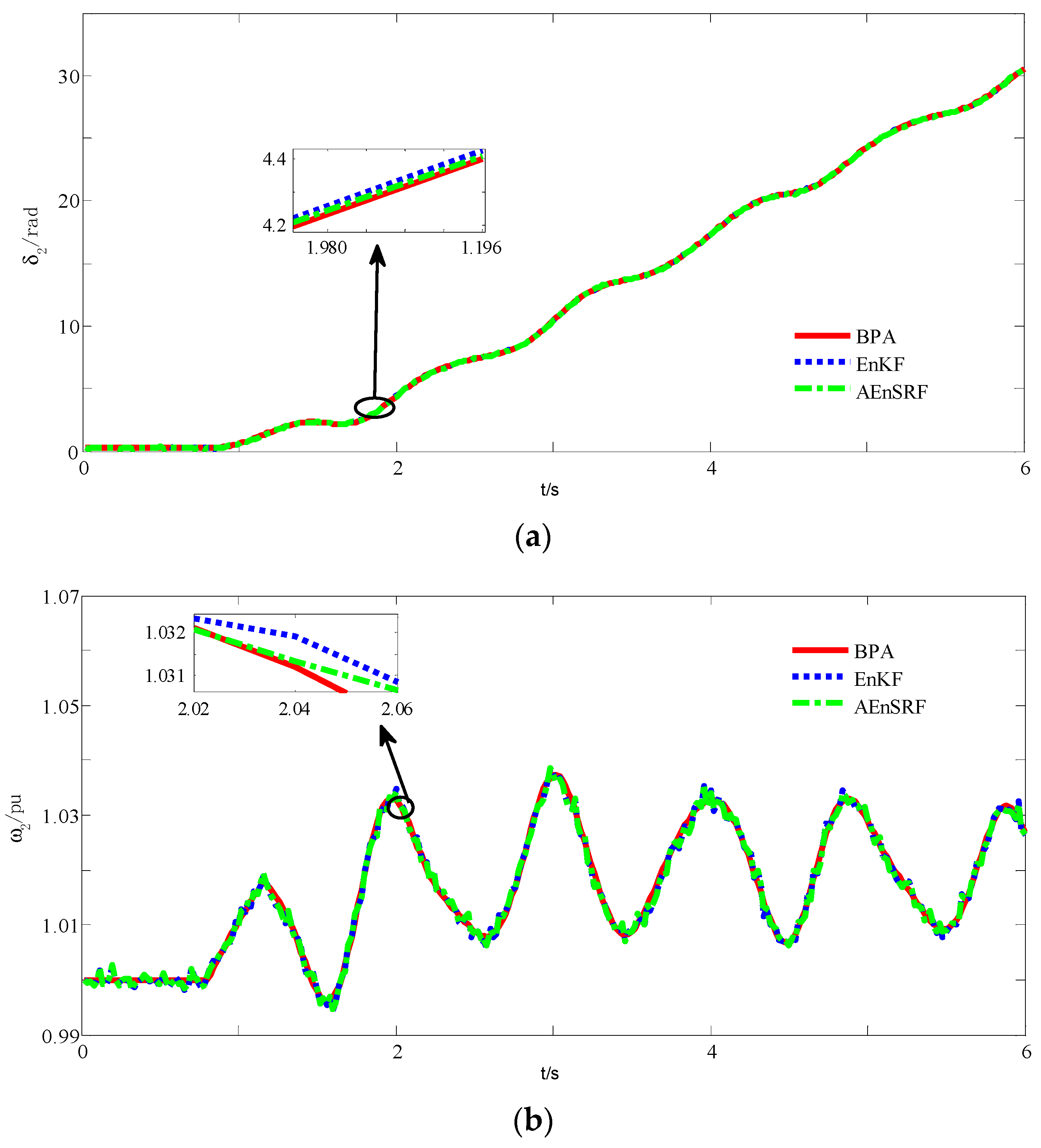
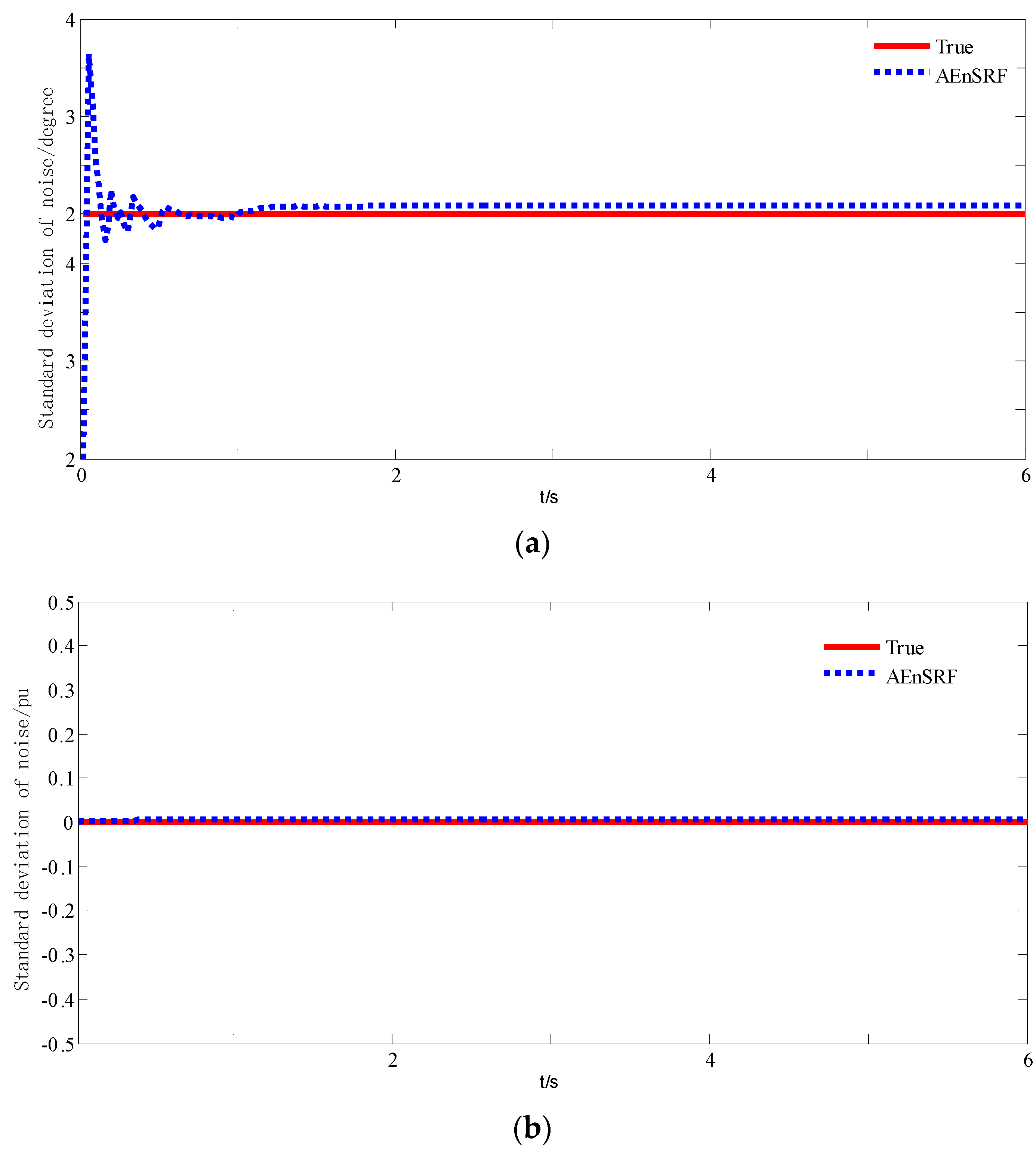
4.1. Basic Test Analysis

The IEEE-9 bus system is firstly taken as the test system in this paper. The single-line diagram of it is given in Figure 2. The classical second-order model of generator considering governor is adopted in simulation. The inertia time constants of G1, G2, and G3 are respectively 47.28, 12.8, 6.02 s; and the damping coefficient is set to 2. The initial values of generator state variables and control variables are set to the values of the system’s stable operation before fault occurred. Suppose that in the IEEE 9 bus system, three-phase short-circuit fault occurs at the beginning of branch 4–8 at 0.8 s. After 0.36 s, the switch on both sides of branch jumps off and the fault is removed. The whole simulation time is 6 s.

The real values of power angle and angular velocity of generator are obtained by Bonneville Power Administration (BPA) simulation software, and the measured values are obtained by adding the real values to the random noise where its mean value obeys normal distribution with zero standard deviation. In this paper, the DSE algorithm is implemented in Matlab. The initial values of the estimated generator state variables are set to stable operation value, and the initial state error covariance matrix is set to unit matrix.

In order to further compare the difference of filtering results of each algorithm, the root mean square error (RMSE) is used

$$RMSE=\sqrt{\frac{1}{n}{\displaystyle \sum _{k=1}^n{({\widehat{X}}_{k|k}-X_k)}^2}}$$

(66)

where $n$ is the sampling period.

The process noise variance matrix and the measurement noise variance matrix of the generator are selected as the corresponding values in [10,11]. Figure 3 is a comparison of the filtering results of G1 by utilizing the EnKF and EnSRF algorithms under normal noise.

Table 1. The RMSE results of EnKF and EnSRF.

Generator Number	Algorithm	$\mathit{\delta }$/rad	$\mathit{\omega }$/pu
G1	EnKF	0.0345	9.7396 $\times {10}^{-4}$
	AEnSRF	0.0329	9.1950 $\times {10}^{-4}$
G2	EnKF	0.0346	10.000 $\times {10}^{-4}$
	AEnSRF	0.0330	9.6680 $\times {10}^{-4}$
G3	EnKF	0.0354	11.000 $\times {10}^{-4}$
	AEnSRF	0.0344	10.000 $\times {10}^{-4}$

gives the RMSE results of EnKF and EnSRF algorithms.

As it might be noted from Figure 3 and Table 1, EnKF and AEnSRF both show good filtering effect without deviation of measurement noise. Because the observation value in AEnSRF does not introduce disturbance, the problem of underestimation in EnKF filtering is avoided. The filtering-precision of AEnSRF is improved comparing with EnKF.

Figure 4 is a sketch of the noise estimator tracking the measured noise in AEnSRF without deviation from the measured noise.

From the simulation, we can see that in the process of tracking power angle measurement noise by AEnSRF, the standard deviation of 0.14 s is stable at 1.9 degrees, and the angular velocity is too small (almost 0). Combining with Figure 4, it can be remarked that AEnSRF can track the measured noise more accurately.

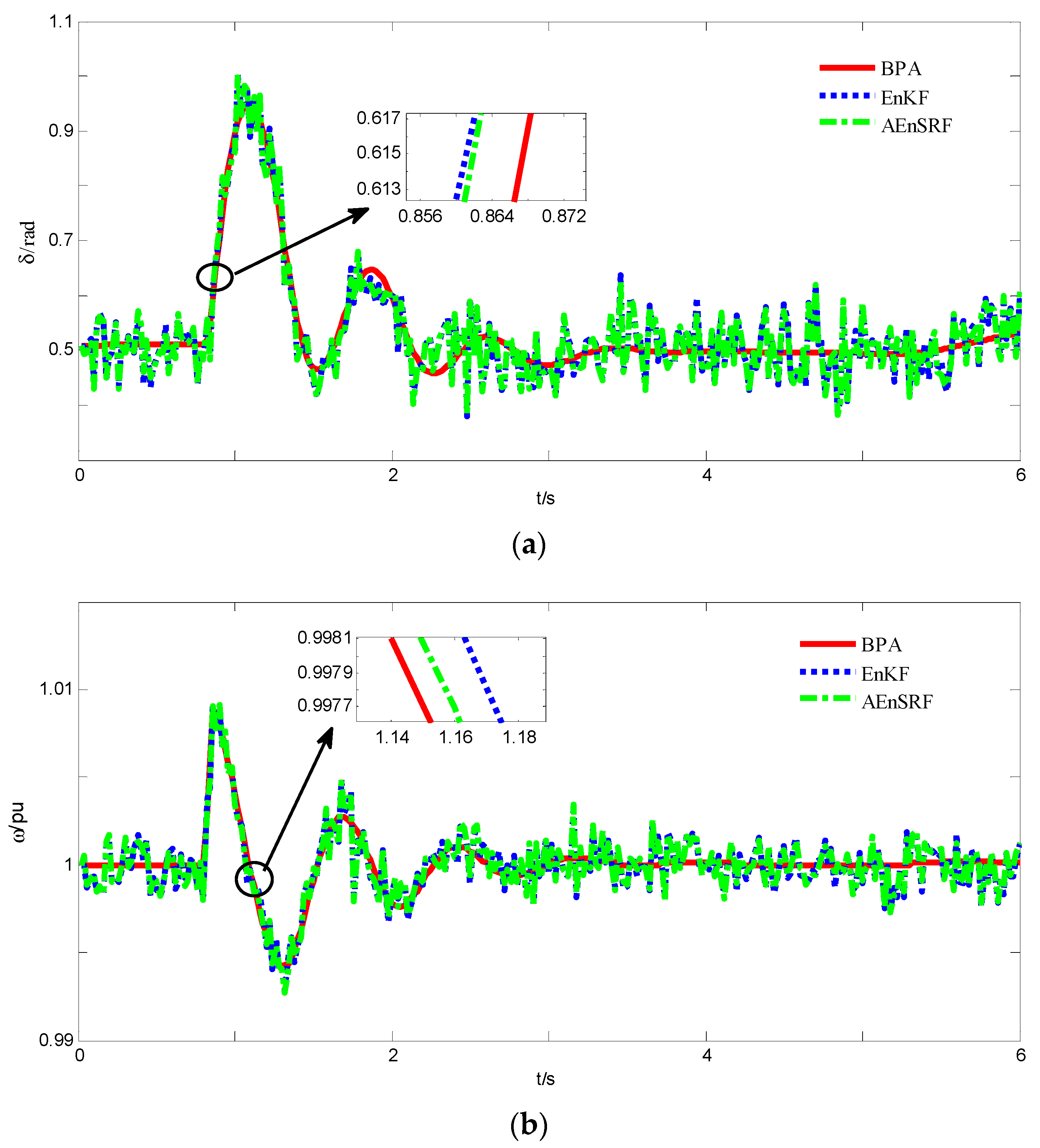
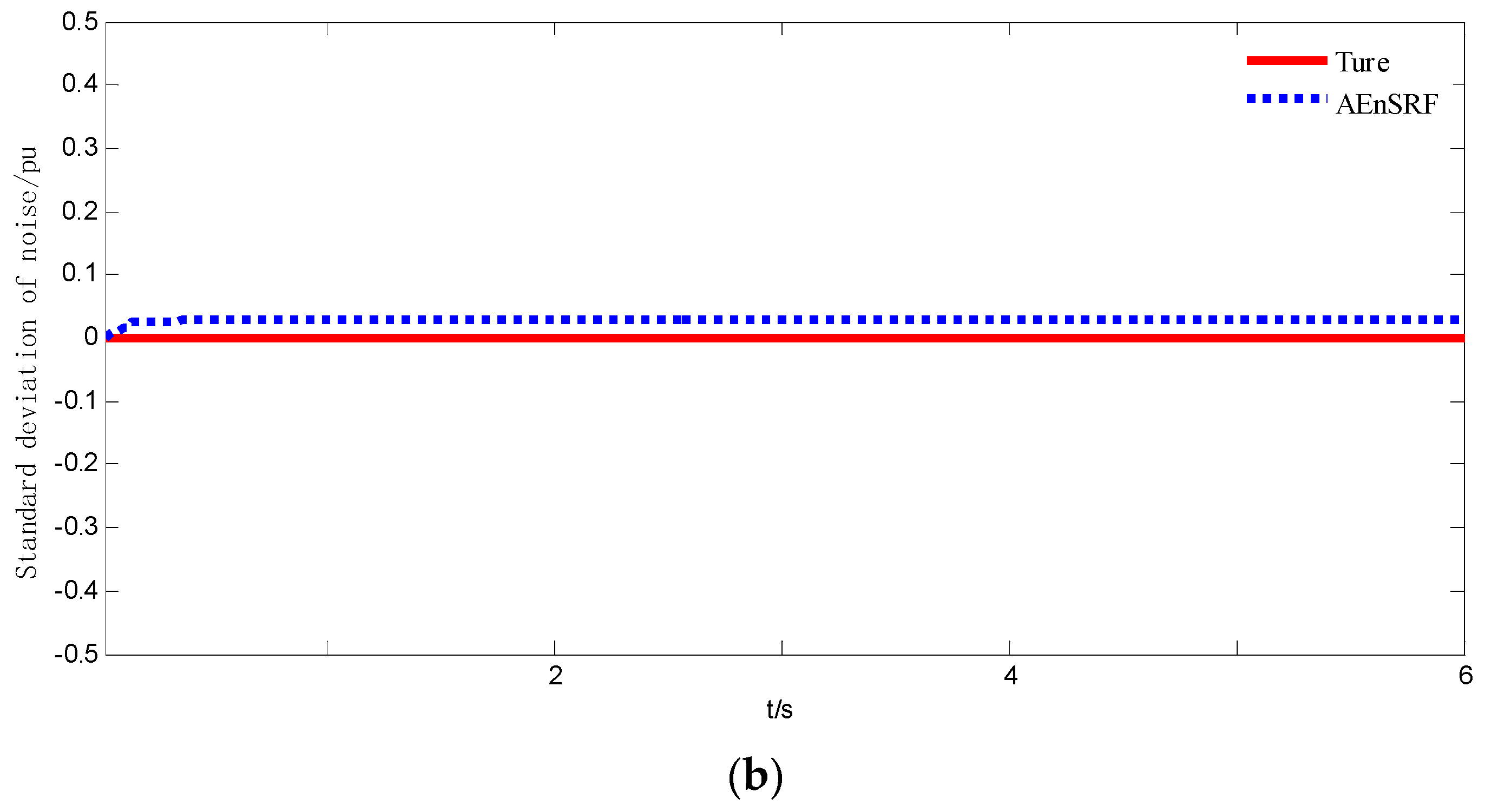
4.2. Noise Measurement and Analysis on the IEEE 9-Bus System

In this subsection, G2 is taken as an example to test the estimation effect of AEnSRF on generator state as well as the tracking of measurement noise when it is biased. Assuming that the actual value of the standard deviation of power angle measurement noise is 3 degrees, the value is set as 2 degrees in the filtering program to detect the tracking effect of AEnSRF on power angle measurement noise.

Figure 5 depicts the comparison results of G2 by utilizing EnKF and AEnSRF algorithms, respectively. It can be obviously noted from Figure 5 that both of them can show good estimation results under the consideration of measurement noise deviation condition.

The simulation results of G2 show that under AEnSRF algorithm, the RMSE of power angle estimation is 0.0516, the RMSE of electric angular velocity estimation is 0.0011. Under EnKF algorithm, the RMSE of power angle estimation is 0.0536 and the RMSE of electric angular velocity estimation is 0.0012. By comparing both algorithms, AEnSRF has higher filtering-precision.

Figure 6 is the simulation diagram of AEnSRF tracking curve for measurement noise when there is a deviation in measurement noise. As it can be noticed from this figure, when the power angle measurement noise is biased, the Sage–Husa noise estimator with on-line real-time estimation noise is introduced by AEnSRF, which makes the estimated standard deviation of power angle measurement noise stabilize around 3 degrees at about 1.1 s.

4.3. Noise Measurement and Analysis on a Real Power System

For further verification of the proposed algorithm’s effectiveness, simulation tests are also carried out on a real power grid system. One generator outgoing circuit has a short-circuit fault, and the generator parameters are based on the actual data. The initial value of the state variable is the steady value, and the initial error covariance matrix is the unit matrix. Assuming that the actual value of the standard deviation of power angle measurement noise is 2.5 degrees, the value is set to 2 degrees in the filtering program.

Comparing EnKF with the proposed method, Figure 7 and Figure 8 show the simulation results of DSE of generator in the presence of measurement noise deviation. The simulation results of G2 illustrate that under the AEnSRF, the RMSE of power angle estimation is 0.0435, the RMSE of electric angular velocity estimation is 0.0010. Under the EnKF, the RMSE of power angle estimation is 0.0438 and the RMSE of electric angular velocity estimation is 0.0013.

Comparing with EnKF, AEnSRF has higher filtering-precision. In AEnSRF, the noise estimator tracks the power angle measurement noise at 0.3 s and stabilizes at about 2.5 degrees. This shows that AEnSRF has a good tracking effect on measurement noise.

5. Conclusions

In this paper, a novel DSE method was proposed based on the EnSRF; a simplified Sage–Husa adaptive Kalman filter with relatively simple principle and good practicability was introduced. In the proposed AEnSRF method, set members were utilized to approximate the posterior distribution of the real state without random disturbance to the measured values. Comparing with EnKF, AEnSRF could enhance the accuracy of filtering. At the same time, Sage–Husa noise estimator was added between the prediction and correction steps to estimate the measurement noise online and in real time, which effectively avoided the problem that the filtering-precision was reduced or even divergent due to the deviation of the measurement noise.

References

1. Wang, Y.; Sun, Y.; Dinavahi, V.; Wang, K.; Nan, D. Robust dynamic state estimation of power system with model uncertainties based on adaptive unscented H infinity filter. IET Gener. Transm. Distrib. 2019, 13, 2455–2463. [Google Scholar] [CrossRef]
2. De La Ree, J.; Centeno, V.; Thorp, J.S.; Phadke, A.G. Synchronized phasor measurement applications in power systems. IEEE Trans. Smart Grid 2010, 1, 20–27. [Google Scholar] [CrossRef]
3. Wang, Y.; Sun, Y.; Dinavahi, V. Robust forecasting-aided state estimation for power system against uncertainties. IEEE Trans. Power Syst. 2019. [Google Scholar] [CrossRef]
4. Singh, H.; Alvarado, L.; Liu, W. Constrained LAV state estimation using penalty functions. IEEE Trans. Power Syst. 2002, 12, 383–388. [Google Scholar] [CrossRef]
5. Mili, L.; Cheniae, M.; Rousseeuw, P. Robust state estimation of electric power systems. IEEE Trans. Circuits Syst. I Fundam. Theory Appl. 2002, 41, 349–358. [Google Scholar] [CrossRef]
6. Ghahremani, E.; Kamwa, I. Dynamic state estimation in power system by applying the extended Kalman filter with unknown inputs to phasor measurements. IEEE Trans. Power Syst. 2011, 26, 2556–2566. [Google Scholar] [CrossRef]
7. Wang, S.; Gao, W.; Meliopoulos, A. An alternative method for power system dynamic state estimation based on unscented transform. IEEE Trans. Power Syst. 2012, 27, 942–950. [Google Scholar] [CrossRef]
8. Qi, J.; Sun, K.; Wang, J.; Liu, H. Dynamic state estimation for multi-machine power system by unscented Kalman filter with enhanced numerical stability. IEEE Trans. Smart Grid 2018, 9, 1184–1196. [Google Scholar] [CrossRef]
9. Arasaratnam, I.; Haykin, S. Cubature Kalman filters. IEEE Trans. Autom. Control 2009, 54, 1251–1269. [Google Scholar] [CrossRef]
10. Arasaratnam, I.; Haykin, S. Cubature Kalman filtering for continuous-discrete systems: Theory and simulations. IEEE Trans. Signal Process. 2010, 58, 4977–4993. [Google Scholar] [CrossRef]
11. Li, Y.; Li, J.; Qi, J.; Chen, L. Robust cubature Kalman filter for dynamic state estimation of synchronous machines under unknown measurement noise statistics. IEEE Access 2019, 7, 29139–29148. [Google Scholar] [CrossRef]
12. Ai, M.; Sun, Y.; Lv, X. Dynamic state estimation for synchronous machines based on interpolation H∞ extended Kalman filter. In Proceedings of the IEEE 33rd Youth Academic Annual Conference of Chinese Association of Automation (YAC), Nanjing, China, 18–20 May 2018. [Google Scholar]
13. Esmaeil, G.; Innocent, K. Online state estimation of a synchronous generator using unscented Kalman filter from phasor measurements units. IEEE Trans. Energy Convers. 2011, 26, 1099–1108. [Google Scholar]
14. Gopinath, G.; Shyama, P. Sensorless control of permanent magnet synchronous motor using square-root cubature Kalman filter. In Proceedings of the IEEE 8th International Power Electronics and Motion Control Conference (IPEMC-ECCE Asia), Hefei, China, 22–26 May 2016. [Google Scholar]
15. Evensen, G. Sequential data assimilation with a nonlinear quasi-geostrophic model using Monte Carlo methods to forecast error statistics. J. Geophys. Res. Ocean. 1994, 106, 10143–10162. [Google Scholar] [CrossRef]
16. Huang, R.; Diao, R.; Li, Y.; Sanchez-Gasca, J.; Huang, Z.; Thomas, B.; Etingov, P.; Kincic, S.; Wang, S.; Fan, R.; et al. Calibrating parameters of power system stability models using advanced ensemble Kalman filter. IEEE Trans. Power Syst. 2018, 33, 2895–2905. [Google Scholar] [CrossRef]
17. Lee, W.; Gim, J.; Chen, M.; Wang, S.; Li, R. Development of a real-time power system dynamic performance monitoring system. IEEE Trans. Ind. Appl. 1997, 33, 1055–1060. [Google Scholar]
18. Gillijns, S.; Mendoza, O.B.; Chandrasekar, J.; De Moor, B.L.R.; Bernstein, D.S.; Ridley, A. What is the ensemble Kalman filter and how well does it work? In Proceedings of the IEEE American Control Conference, Minneapolis, MN, USA, 14–16 June 2006. [Google Scholar]
19. Kotecha, J.; Djuric, P. Gaussian particle filtering. IEEE Trans. Signal Process. 2003, 51, 2592–2601. [Google Scholar] [CrossRef]
20. Fan, R.; Huang, R.; Diao, R. Gaussian mixture model-based ensemble Kalman filter for machine parameter calibration. IEEE Trans. Energy Convers. 2018, 33, 1597–1599. [Google Scholar] [CrossRef]
21. Fan, R.; Liu, Y.; Huang, R.; Diao, R.; Wang, S. Precise fault location on transmission lines using ensemble Kalman filter. IEEE Trans. Power Del. 2018, 33, 3252–3255. [Google Scholar] [CrossRef]
22. Burgers, G.; Peter, J.; Evensen, G. Analysis scheme in the ensemble Kalman filter. Mon. Weather Rev. 1998, 126, 1719–1724. [Google Scholar] [CrossRef]
23. Whitaker, J.S.; Hamill, T.M. Ensemble data assimilation without perturbed observations. Mon. Weather Rev. 2003, 130, 1913–1924. [Google Scholar] [CrossRef]
24. Tippett, M.K.; Anderson, J.L.; Bishop, C.H.; Hamill, T.M.; Whitaker, J.S. Ensemble square root filters. Mon. Weather Rev. 2003, 131, 1485–1490. [Google Scholar] [CrossRef]
25. Zhu, Z.; Liu, S.; Zhang, B. An improved Sage-Husa adaptive filtering algorithm. In Proceedings of the IEEE 31st Chinese Control Conference, Hefei, China, 25–27 July 2012. [Google Scholar]
26. Wang., Y.; Sun, Y.; Dinavahi, V.; Cao, S.; Hou, D. Adaptive robust cubature Kalman filter for power system dynamic state estimation against outliers. IEEE Access 2019, 7, 105872–105881. [Google Scholar] [CrossRef]
27. Deng, F.; Chen, J.; Chen, C. Adaptive unscented Kalman filter for parameter and state estimation of nonlinear high-speed objects. J. Syst. Eng. Electron. 2013, 24, 655–665. [Google Scholar] [CrossRef] [Green Version]
Figure 1. The flowchart of adaptive ensemble square root Kalman filter (AEnSRF) algorithm.
Applsci 09 05200 g001
Figure 2. The single-line diagram of IEEE-9 bus test system.
Applsci 09 05200 g002
Figure 3. Comparison of G1 state filtering results under ensemble Kalman filter (EnKF) and AEnSRF: (a) Power angle dynamic estimation curve of G1; (b) electric angular velocity dynamic estimation curve of G1.
Applsci 09 05200 g003aApplsci 09 05200 g003b
Figure 4. Measurement noise tracking curve of G1 under AEnSRF: (a) Power angle measurement noise tracking curve of G1; (b) angular velocity measurement noise tracking curve of G1.
Applsci 09 05200 g004
Figure 5. Comparisons of G2 state filtering results between EnKF and AEnSRF in the presence of measurement noise deviation: (a) Power angle dynamic estimation curve of G2; (b) electric angular velocity dynamic estimation curve of G2.
Applsci 09 05200 g005
Figure 6. Tracking curve of G2 measurement noise by AEnSRF in the case of measurement noise deviation: (a) Power angle measurement noise tracking curve of G2; (b) angular velocity measurement noise tracking curve of G2.
Applsci 09 05200 g006
Figure 7. Contrast chart of EnKF and AEnSRF for generator state filtering with deviation of measurement noise: (a) Power angle dynamic estimation curve of generator; (b) dynamic angular velocity estimation curve of generator.
Applsci 09 05200 g007
Figure 8. Tracking curve of AEnSRF for generator measurement noise with deviation of measurement noise: (a) Power angle measurement noise tracking curve of generator; (b) angular velocity measurement noise tracking curve of generator.
Applsci 09 05200 g008aApplsci 09 05200 g008b