Abstract
Using a single-point sensor, non-intrusive load monitoring (NILM) discerns the individual electrical appliances of a residential or commercial building by disaggregating the accumulated energy consumption data without accessing to the individual components. To classify devices, potential features need to be extracted from the electrical signatures. In this article, a novel features extraction method based on current shapelets is proposed. Time-series current shapelets are determined from the normalized current data recorded from different devices. In general, shapelets can be defined as the subsequences constituting the most distinguished shapes of a time-series sequence from a particular class and can be used to discern the class among many subsequences from different classes. In this work, current envelopes are determined from the original current data by locating and connecting the peak points for each sample. Then, a unique approach is proposed to extract shapelets from the starting phase (device is turned on) of the time-series current envelopes. Subsequences windowed from the starting moment to a few seconds of stable device operation are taken into account. Based on these shapelets, a multi-class classification model consisting of five different supervised algorithms is developed. The performance evaluations corroborate the efficacy of the proposed framework.
1. Introduction
The rapid growth of economic development has drastically increased electricity energy demands over the last few years. In order to meet this emerging growth, most electric utilities are upgrading their traditional power grids to more sophisticated, technically prudent and self-healing smart grid technologies [1]. It is now possible to monitor, manage and control the electricity energy demands on real time usage basis to enhance the efficiency of a power system network. For a substantial smart energy management framework, a reliable appliance load monitoring (ALM) system is important, which can ensure most risk-free and cost-effective energy consumption for the users. However, ALM can be executed by intrusive load monitoring (ILM) techniques that are relatively more accurate but require more sensing and measuring equipments and resources [1]. Another more immaculate way to execute ALM with less measuring device requirements is non-intrusive load monitoring (NILM). Non-intrusive appliance load monitoring (NIALM) or NILM determines individual energy consumption profile of different electrical appliances using a single measurement point. In the age of emerging smart grid technologies, sophisticated home energy management systems and efficacious utility infrastructures, NILM yields to be a crucial tool for reliable and inexpensive smart metering systems.
The concept of NILM was first introduced by George W. Hart [2]. NILM methods for analyzing the energy signatures are based on three primary approaches—steady-state analysis, transient-state analysis and non-traditional appliance features [1,2,3,4]. The steady-state analysis detects the changes in load identification considering stable states of devices, while the transient-state analysis focuses on the transitional states in energy consumption profile. The last approach concentrates on determining non-typical features of the electrical devices to disaggregate them. The detailed comparative study of these three NILM approaches is reported in [1,3,4].
NILM analyzes aggregate electrical load data together with appliance profile data to decompose the aggregate load into a family of appliance loads that can explain its characteristics [5]. From the inception of this concept, different methodologies have been and are being proposed to get significant improvement in reliable load monitoring and identification premises. To identify devices correctly, potential signatures extraction from the load data is necessary. Hence a novel non-intrusive load signatures extraction technique is proposed in [6], which first selects the candidate events that are likely to be associated with the appliance by using generic signatures and an event filtration step. It then applies a clustering algorithm to identify the authentic events of this appliance and in the third step, the operation cycles of appliances are estimated using an association algorithm. Another new concept of NILM techniques is presented in [7], where wavelet design and machine learning are applied. In this work, the wavelet coefficients of length-6 filter are determined employing procrustes analysis and are used to construct new wavelets to match the load signals. The newly designed wavelets are applied to a test system consisting of four loads and an improved prediction accuracy is observed comparing with the traditional wavelets based method. However, another wavelets based method reporting application of power spectrum of wavelet transform coefficients (WTCs) for load monitoring and identification is documented in [8]. Continuous wavelet transform (CWT) analysis to find feature vectors for switching voltage transients for NILM is discussed in [9], where support vector machines (SVMs) are trained by these features to identify loads. Orthogonal wavelet based NILM methodology is proposed in [10], where supervised and semi-supervised classifiers are used to automate the load disaggregation process.
Most of the efforts attempt to disaggregate loads yield low sampling frequencies and steady consumption states. To achieve a better accuracy, it is necessary to consider higher sampling frequencies and both steady states and transient states. In regard to this phenomenon, a novel event-based detector for NILM applications is reported in [11]. This method takes into account small power changes which are not usually well detected on most low-frequency systems and it is based on the application of Hilbert transform to obtain the envelope of the signal.
Microscopic characteristics collected from current and voltage measurements are employed to detect electrical devices in [12]. Another novel approach based on linear-chain conditional random fields (CRFs) combining current and real power signatures for efficient NILM solution is reported in [13]. Phase noise of individual device as a new load signature characteristic is discussed in [14]. However, a novel particle-based distribution truncation method with a duration dependent hidden semi-Markov model for NILM is presented in [15]. In [16], gated linear unit convolutional layers are used to extract information from the sequences of aggregate electricity consumption. Residual blocks are also introduced to refine the output of the neural network in where the partially overlapped output sequences are averaged to produce the final output of the model. However, a number of intricate signal processing techniques based NILM solutions are proposed in [17,18,19,20,21]. A few works on NILM applying computationally complicated deep learning techniques are documented in [22,23,24,25,26,27,28,29]. A demand side personalised recommendation system (PRS) is proposed in [30] that employs service recommendation techniques to infer residential users’ potential interests and needs on energy saving appliances. The proposed scheme starts with the application of an NILM method based on generalised particle filtering to disaggregate the end users’ household appliance utilisation profiles achieved from the smart meter data. Then, based on the NILM results, several inference rules are applied to infer the preferences and energy consumption patterns. In [31], an improved NILM technique is proposed, which comprises a shunt passive filter installed at the source side of any residential complex. The first step is to determine the harmonic impedance at the load side for different groups of loads for a single household, whereas the second step is to implement a fuzzy rule-based approach for identification of different loads at the consumer end. In [32], a statistical features based NILM solution is proposed, which applies a number of supervised classifiers on current measurements and evaluates performance comparison for device disaggregation.
From the literature review, it is yielded that different novel and sophisticated analysis methodologies are proposed till date for efficient NILM solutions. This article proposes another novel approach for features extraction from the load signatures, referred to as current shapelets. Shapelets are generally defined as interpretable time-series subsequences of a dataset, which can categorize an unlabeled sequence if it comprises an occurrence of the shapelets within a specified learning distance. The fundamental concepts of shapelets are elucidated in [33,34,35]. Shapelets are utilized by many researchers in computer science and engineering to develop robust, compact and fast classification models. However, in this work, the analysis starts with a keen observation of the normalized current data of the devices present in the controlled on/off loads library (COOLL) NILM public domain dataset [36]. A 5-point moving average filter is applied to remove high frequency spikes. Electrical devices can be turned on or off at any time instant. When a device is turned on, there happens to be a prominent change in the current value and a peak point is reached. This is true for each cycle of operation. After a few instants, the current becomes stabilized, which can be inferred as the stable phase of a device current. Current envelopes are formed by locating and connecting the local maxima at each cycle of device operation. The time window length of these envelopes is shorter than that of original current signatures, as the envelopes initiate from the moment when a device is turned on and end at a stable point of operation. From these envelopes, time-series shapelets are determined, which provide feature components to identify devices.
In COOLL public NILM dataset, there are 42 devices of different brands and power ratings. Each device has 20 instances of data sets; hence there are 840 datasets in the entire database. Current and voltage data of 6 s are recorded with a sampling frequency of 100 kHz. This work focuses on the current signatures of the devices, since the variations in current data are more prominent than those in voltage signatures. However, the devices are of major residential load types. The device types and number of each type are as follows—Drill (6), Fan (2), Grinder (2), Hair Dryer (4), Hedge Trimmer (3), Lamp (4), Paint Stripper (1), Planer (1), Router (1), Sander (3), Saw (8) and Vacuum Cleaner (7).
The developed classification model has 12 classes, which correspond to the types of device instances in COOLL database. The model comprises five supervised learning algorithms—ensemble, binary decision tree (DT), discriminant analysis, naïve Bayes and k-nearest neighbors (k-NN). 80% of the database is employed as the training data, whereas 20% is employed as the testing data. The proposed system is tested in MATLAB®. A comparative study on the classification performance of the applied algorithms is presented in this paper. The most accurate classification results of the proposed multi-class system are obtained for ensemble, in where the training accuracy is 100% and the testing accuracy is more than 95%.
The major contributions of this work are as follows.
- Determines current envelopes from the original normalized signatures.
- Introduces a concept of features extraction by determining time-series shapelets from the envelopes based on a unique searching and matching technique. This technique depends on an implicit analysis of the fundamental behavior of device current.
- Develops a multi-class classification model trained and tested by these current shapelets.
The remainder of the manuscript is organized as follows. Section 2 explains the proposed method, in where time-series shapelets are briefly explained and the implemented shapelets extraction method is described. Section 3 subsumes the experiments and results, in where the supervised learning methods are studied and different casework analyses are reported to present the performance evaluations of the developed device classification model. Section 4 briefly presents the specific contributions and future prospects of the proposed work. Finally, Section 5 concludes the article.
2. Proposed Method
The proposed NILM solution is developed utilizing time-series shapelets for device classification. The fundamental concepts of shapelets and related definitions are documented in Section 2.1. The implemented methodology for determining shapelets is articulated in Section 2.2.
2.1. Time-Series Shapelets
Time-series shapelets are defined as subsequences or snippets in a time-series dataset, which are directly interpretable and can be represented as class members in a classification problem domain [33,34,35]. Shapelets are used to classify any unlabeled time-series data sequence that contains an occurrence of the shapelets within some previously learned distance thresholds [34]. The application of shapelets is relatively a new concept in classification problem solution approaches, especially shapelets are used by many practitioners in computer science for comparatively robust, fast and compact classification performances. Shapelets are basically local features in a time-bounded sequence, which can give insights on the premises of differences between two classes. Some necessary definitions [33,34,35] to understand the state-of-the-art are provided in the following.
2.1.1. Time-Series Sequence
A time-series sequence is an ordered set of r real-valued variables. Data points are typically arranged by temporal order, which are spaced at equal time intervals.
2.1.2. Subsequence
Given a time-series sequence of length r, a subsequence is a set of contiguous data samples of length , that is , for . In a classification framework, all the subsequences of all possible lengths need to be extracted to find out the best subsequences, which can distinguish the target classes most significantly.
2.1.3. Sliding Window
All possible subsequences of length m in a time-series sequence of length r can be extracted by sliding a window of size m across , where each subsequence can be denoted as . Here p represents the starting index of the subsequence.
2.1.4. Distance
The similarity measurement of a subsequence with a time-series sequence is determined by calculating distance, as expressed in the following.
This is the actual distance between the subsequence and its best matching location in the sequence. Here i denotes the beginning of the m-length sliding window in , where the subsequence is checked for its best match. The peak value of i can be . However, in this work, a slightly modified formula to measure the distance is used. The modified formula and its significance are explained in the later Subsection.
2.2. Shapelets Extraction in This Work
In a standard practice of shapelets based classification, firstly best shapelets of any group of data, which may occur at anywhere of a time series sequence having different lengths, are found out using different searching algorithms and advanced techniques [33,34,35]. Then, these shapelets are matched with a set of long data. All possible subsequences are considered as potential candidates whose minimum distances to all training datasets are fed to the predictor for training as predictor features to rank the accuracy of the candidates. Because of this high number of candidates, runtime of shapelets determination may not be promising in many real-world applications like NILM. As a time-effective solution, in this work a unique approach is proposed to extract shapelets from the starting phase of the time-series device current signatures. It is implied that here starting position means the moment of initiating the on-state of a device. It is shown that the current dataset contains most of its useful and distinguishable informative features at the beginning of its emergence. Thus, shapelets are determined from an initial phase of the data spanning from the state of commencement to some distant position. In the proposed method, shapelets are matched with the exact starting position or very close to the starting position of the sequence. Thereby, shapelets selection from a shorter length sequence reduces the time and complexity of execution.
The proposed shapelets determination process starts with implicitly analyzing current signatures of the device instances present in COOLL database. Figure 1 presents normalized current data recorded from a particular device operation. A symmetrical alternating current having sinusoidal form repeats the same shape at the fixed interval of time even after addition of harmonics. Taking into account this fact, the time-series shapelets from the current data are determined using envelopes of the current rather than the original signature. Here, current envelopes are produced by taking the local maxima (peak) at each cycle of the data and then, those peak points are connected with each other.
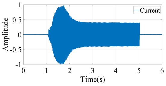
Figure 1.
Normalized current signature of a particular device in COOLL database.
Figure 2 presents the envelope and subsequence of the envelope of the current shown in Figure 1. In this figure, horizontal axis represents the index number of the envelope, where index 1 denotes the starting moment of the device. Since, only the local maxima of each cycle are considered and the fundamental line frequency here is 60 Hz, the difference between any two adjacent indexes in time is 16.67 ms. However, this index is used to represent the length, beginning of subsequences in the rest of the article.
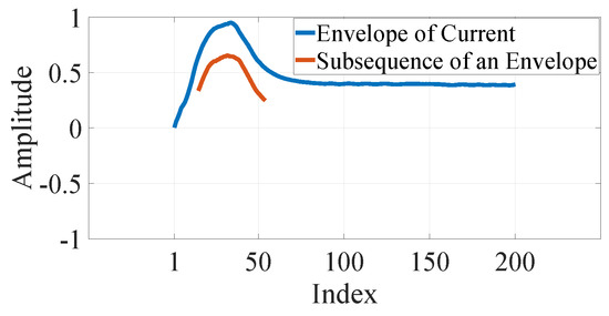
Figure 2.
Envelope and subsequence of the envelope extracted from the current shown in Figure 1.
In Figure 2, a subsequence of the envelope is shown being placed at the best matching position with the envelope. Here, the beginning index of the subsequence p is 15 and the length m is 40. In other words, it begins after ms from the starting moment of the current of the device and has a time span of ms.
Electrical devices can be turned on or off at any time instant. When a device is turned on, there happens to be a prominent change in the current value and a peak point is reached. This is true for each cycle. After a few instants, the current becomes stabilized, which can be inferred as the stable phase of a device current. Therefore, in this work, shapelets are searched and extracted from the first few seconds of a device operation instead of the entire time frame. For a shapelet, to find the best matching distances against different current envelopes, this paper proposes to restrict the movement of the sliding window within the first few seconds resulting in , where . The distance between a subsequence and its best matching location is modified in this work as follows.
Here, and . The two average terms are used to shift the active portion of time-series sequence (envelope) and the associated subsequence to the same DC level. The underlying reason behind modifying (1) to get (2) is embedded into an anticipation of device operational characteristics. Since, current data from different devices are experimented to strive for accusation from a single point sensor for NILM, it may generally happen that when a device gets started, already another device is running implying that it has already been drawing current for itself. Thereby, the current of the new device would add to the current from the already running device. Now, if the shapelet from the same type of device is matched with this current, it would hardly produce convincing results. Hence, the DC levels of both the active sequence (envelope) and subsequence are made same at first, while calculating the distance.
There is an inherent advantage of conceptualizing and applying (2) rather than (1) to measure the distance between any subsequence and its best matching location in a time-series. (2) provides the flexibility to handle high power devices with equal footing of low power devices. It can be implied that current envelopes from a high power appliance would have higher level of DC value, but since (2) is used in this work making both the subsequence and the time-series being matched at the same DC level, a high power device will not be of any difference compared to a low power device. Thereby, the analysis works fine for any power appliances.
In this work, partial shapelets or partial distance measurements in the current data are not considered. Partial shapelets are assumed as components or segments of any particular shapelet. Based on the operatives of electrical appliances, it can be asserted that after the start (turn on) of any device, the shape of a current envelope of the next few seconds holds the distinguishing feature of that particular device. Then, the question of partial shapelet may arise only if few seconds of current are not available, implying that the device is already turned off. In that case, there is no need to identify the load in real-time application, which is supposed to be turned on for such a short period of time. Another perspective of not analyzing partial segments in a shapelet relates to unusual and momentary changes in the measurement. There may be some sharp rise or fall in current for very short intervals due to the faults or glitches in the power line. It will be unwise to try to disaggregate any load based on those impulsive changes.
3. Experiments and Results
A classification model based on the shapelets from the current envelopes is developed to disaggregate the appliances and categorize them into different classes. The developed classification model has 12 classes with a training dataset constituting 80% of the entire database and a testing dataset constituting 20% of the entire database. This work investigates five supervised classification algorithms. Section 3.1 articulates the study of the applied classification methods. Section 3.2 describes the classification performance analysis.
3.1. Study of the Applied Classifiers
The study of the supervised classification algorithms is briefly reported in the following.
3.1.1. Naïve Bayes
Naïve Bayes methods are a set of supervised learning algorithms based on applying Bayes theorem with the “naïve” assumption of conditional independence between every pair of features given the value of the class variable [37]. According to [37], for a given class variable Y and dependent feature vector through Bayes theorem states that
Applying the conditional independence assumption which implies that
For all j, the relationship can be simplified as
Naïve Bayes classifiers tend to yield posterior distributions that are robust to biased class density estimates, particularly where the posterior is 0.5 (the decision boundary) [38]. Naïve Bayes classifiers assign observations to the most probable class and the algorithm can be explicitly described as follows [38]:
- Estimates the densities of the predictors within each class.
- Models posterior probabilities according to Bayes rule. For all , it can be mathematically expressed as:here Y denotes the class index of an observation, are the random predictors of an observation and represents the prior probability that a class index is k.
- Classifies an observation by estimating the posterior probability for each class, and then assigns the observation to the class yielding the maximum posterior probability.
If the predictors constitute a multinomial distribution, then the posterior probability
where is defined as the probability mass function [38]. Naïve Bayes classifiers require a small amount of training data to estimate the necessary parameters [37]. These classifiers can be extremely fast compared to more sophisticated methods, since the decoupling of the class conditional feature distributions means that each distribution can be independently estimated as a one dimensional distribution [37]. Thereby the problems associated with dimensionality can be alleviated.
3.1.2. Discriminant Analysis
Linear discriminant analysis (LDA) and quadratic discriminant analysis (QDA) are two classic methods of classification for multi-class systems having closed form solutions, which can be easily computed [37]. In this work, LDA is applied. According to [37], LDA can be mathematically formulated from probabilistic models, which characterize the class conditional distribution of a sample data for each class k. Using Bayes theorem,
here class k is selected, which maximizes this conditional probability. According to [37], for a more specific application of LDA, is modeled as a multivariate Gaussian distribution with density, which can be expressed as:
here d is the number of features and denotes the class means. For LDA, the Gaussians for each class are assumed to share the same covariance matrix: [37].
3.1.3. Ensemble
Ensemble methods combine the predictions of several base estimators built with a given learning algorithm in order to improve robustness over a single estimator [37]. There are two families of ensemble methods—averaging methods and boosting methods [37]. The basic principle of averaging methods is to develop several estimators independently and then to average their predictions [37]. In this work an averaging method named random forest (RF) classifier is applied. RF is a classifier consisting of a collection of tree-structured classifiers where denotes independent identically distributed random vectors and each tree casts a unit vote for the most popular class at input x [39]. In RF algorithm each tree in the ensemble is built from a sample drawn with replacement from the training set [37,39]. In addition, when splitting a node during the construction of the tree, the split that is chosen is no longer the best split among all features whereas the split that is picked is the best split among a random subset of the features [37,39]. As a consequence of this randomness, the bias of the forest usually slightly increases but, due to averaging, its variance also decreases, usually more than compensating for the increase in bias, hence yielding an overall better model [37,39].
According to [39], for an ensemble of classifiers and with a training set of random vectors , the margin function can be defined as:
here denotes the average number of votes at and is the indicator function. The larger the margin is, the more confidence lies in the classification. According to [39], the generalization error is determined as:
here is the probability over space. For RF classifiers, and according to [31], with the increase in tree numbers it becomes converges to
3.1.4. Binary Decision Tree
Decision trees (DTs) are a non-parametric supervised learning method which creates a model that predicts the value of a target variable by learning simple decision rules inferred from the data features [37]. The premier advantages of DTs are: they require little data preparation, they are able to handle both numerical and categorical data, the cost of predicting data is logarithmic in the number of data points used to train the tree model, and they can handle multi-output problems [37]. However, there are a few disadvantages of DTs: they can create over-complex trees that do not generalize the data effectively, they can be unstable due to small variations in the data, and they create biased trees if some classes dominate [37].
Binary DT classifier is capable of multi-class classification on a sample distribution. The detailed mathematical formulation of DT learning method is articulated in [37]. To characterize the classification criteria, if the outcome takes on values , for node m representing a region with observations and given training vectors and a label vector y, let us consider
be the proportion of class k observations in node m. Common measures of impurity are defined as—
Gini:
Entropy:
and Misclassification:
where is an impunity function and is the training data in node m [37].
3.1.5. k-NN Classifier
Neighbors-based classification is a type of instance-based learning, which does not construct a general internal model, but simply stores instances of the training data [37]. Classification is computed from a majority vote of the nearest neighbors of each point. A query point is assigned the data class, which has the most representatives within the nearest neighbors of the particular point [37]. k-nearest neighbors (k-NN) algorithm is the most common technique to implement nearest neighbors classification in where k is an integer value. However, the optimal choice of the value of k is highly data-dependent [37].
Various metrics are evaluated to determine the distance to categorize query points in a training dataset [40,41,42]. As an instance, a -by-h data sample X, which can be treated as (1-by-h) row vectors and a -by-h data sample Y, which can be treated as (1-by-h) row vectors; different distance metrics between and are defined as follows.
- Euclidean Distance
- Standardized Euclidean Distancehere V is the h-by-h diagonal matrix.
- Mahalanobis Distancehere C is the covariance matrix.
- City Block Distance
- Minkowski Distance
- Chebychev Distance
- Cosine Distance
- Correlation Distancehere and .
- Hamming Distance
- Jaccard Distance
- Spearman Distancehere and are the coordinate-wise rank vectors of and , respectively. and .
Exhaustive search algorithm is applied to find k-nearest neighbors if the following criteria are satisfied.
- Number of columns in X is more than 10.
- X is sparse.
- The distance matrix is any of—, , , , , and .
-tree search algorithm is applied to find k-nearest neighbors if the following criteria are satisfied.
- Number of columns in X is less than 10.
- X is not sparse.
- The distance matrix is any of—, , and .
The detailed analysis of k-NN and other nearest neighbors algorithms are reported in [40,41,42].
In general, classification model parameters are determined by fitting obtained data to the predicted model response. The order is an index representing the flexibility of a model- higher the order, more flexible the model would be. With an increased order, the propensity of fitting the observed data more accurately increases. On the other hand, flexibility contradicts with the certainty in the estimates and this uncertainty is measured by a higher value of variance error. However, a model with low order yields to greater system computational errors, referred to as bias errors. Therefore, it is required to maintain a tradeoff between bias error and variance error. In this research work, MATLAB® library functions are used to implement the supervised learning algorithms, which optimize bias-variance tradeoff characterization and avoid overfitting of the training dataset. In addition, regularization technique is used for preventing overfitting in a predictive model. Generally, regularization techniques specify constraints on the flexibility of a model and reduce uncertainty in the estimates, which provide better scopes for maintaining bias-variance tradeoff. There are a number of regularization algorithms in machine learning. In this work, ridge regression algorithm is used for regularization. Typically, cross-validation tests are carried out to investigate the bias-variance tradeoff. In the proposed work, cross validation losses are computed and no overfitting is observed. The detailed numeric analyses of the classification performance are reported in the next Subsection.
3.2. Performance Analysis
The device classification model trained by current shapelets is assessed to evaluate the efficacy of the proposed framework. There are five test scenarios in this analysis. Classification accuracies are calculated for the applied learning algorithms considering variations in length of shapelets m, beginning point of subsequences p and peak value of sequence index . The test scenarios are explained in the following.
3.2.1. Test Scenario-1
Figure 3 presents the computed classification (testing) accuracies of the applied algorithms for different lengths of shapelets considering p as 1, 5, 9 and 19, respectively, while keeping . Here, legends represent- Ensemble, binary decision tree (DT), discriminant analysis (DA), naïve Bayes (NB) and k-nearest neighbors (k-NN).
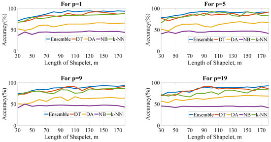
Figure 3.
Accuracy vs length of shapelets for and different values of p for different classifiers.
It is evident from Figure 3 that accuracy of any classifier is comparatively low when the length m of the shapelets is 30. As the length increases upto 90, accuracy tends to increase at first. But, after 130, there seems no significant increase in accuracy with the increase in the value of m. Therefore, it can be implied that the searching region for evaluating subsequences can be confined within 90 to 130 of m. Also, it can be noticed that ensemble classifier gives better result for most of the time.
3.2.2. Test Scenario-2
Figure 4 presents the computed classification (testing) accuracies for each learning algorithm with different p values in the horizontal axis. Here, the length of the shapelets m is variable (shown in the legends) and is kept constant as 15. The objective of this test casework is to show the trend of accuracy with respect to p for different algorithms. It is evident that there is a trend of decreasing accuracy as the value of p increases signifying that the most distinctive subsequence resides in the starting region of any device. Therefore, it is suggested that the boundary to locate the subsequences should be confined near the starting point of a device operation.
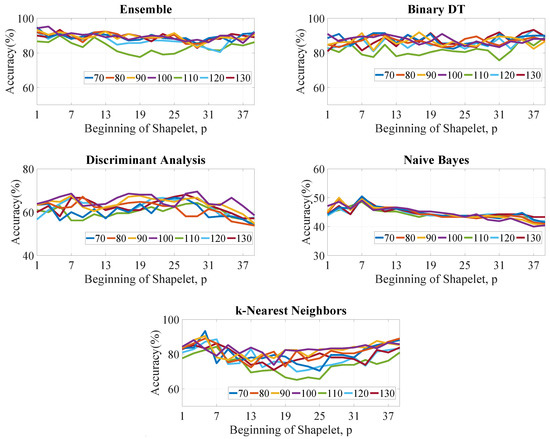
Figure 4.
Accuracy vs the beginning point p for for different classifiers considering different values of m (legends).
3.2.3. Test Scenario-3
Figure 5 presents the computed testing accuracies of ensemble and binary DT algorithms for with length of the shapelets in the horizontal axis. In this case, is selected as either 15 or 60. It can be noticed that different does not yield significantly different results. Therefore, a question may arise over the selection of value. For this selection process, analysis of accuracy obtained for ensemble algorithm for different values of p, and m is carried out here. Ensemble classifier is chosen because it provides better results than other methods.
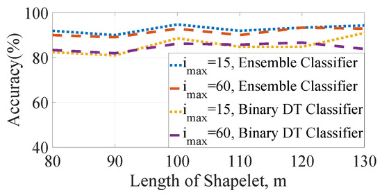
Figure 5.
Accuracy vs length of shapelets for ensemble and binary DT for and & 60.
Figure 6 presents classification accuracies of ensemble computed for different values of p and & 60 with lengths of shapelets , 90, 100, 110, 120 & 130, respectively. It can be noticed that for , the accuracy curves obtained for & 60 in each case are pretty similar. Therefore, it is suggested that should be slightly greater than or equal to 15. For the further performance evaluations in this article, is selected as 15.
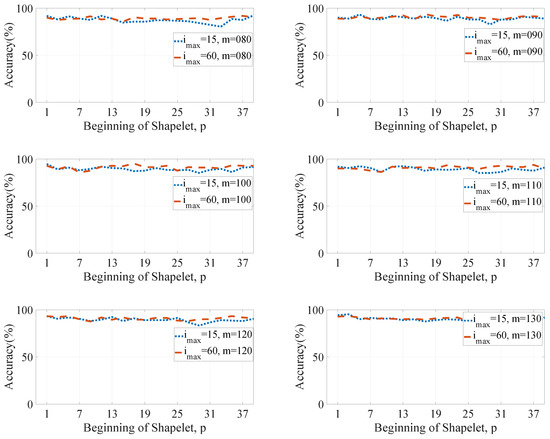
Figure 6.
Accuracy vs p values for & 60 with different values of m (ensemble).
3.2.4. Test Scenario-4
This casework is segmented into two parts—training results and testing results. Table 1 and Table 2 show the training accuracies measured for each classifier for different lengths of shapelets for , and , , respectively. From Table 1, it is evident that ensemble and k-NN identify all the devices correctly for and each length. From Table 2, it can be stated that ensemble outperforms other methods by identifying all the devices correctly for .

Table 1.
Training Accuracies (%) of the Classifiers for , .
Table 2.
Training Accuracies (%) of the Classifiers for , .
Table 3 and Table 4 show the testing results comprising accuracy values and associated 10-fold cross-validation losses for different lengths of shapelets with , and , , respectively. From Table 3, it is evident that for and , ensemble produces the best classification accuracy of more than 95% with the least cross-validation loss of . From Table 4, it can be observed that for and , the best classification accuracy of more than 94% with the least cross-validation loss of is obtained for ensemble. In Table 1, Table 2, Table 3 and Table 4, DT stands for binary DT, DA stands for discriminant analysis and NB denotes naïve Bayes algorithm.
Table 3.
Testing Accuracies (%) of the Classifiers for , .
Table 4.
Testing Accuracies (%) of the Classifiers for , .
3.2.5. Test Scenario-5
A more detailed performance analysis of the device classification model based on the current shapelets is carried out using confusion matrices calculated for the applied classifiers. From Table 1, Table 2, Table 3 and Table 4, it can be implied that the best classification results are obtained for the setup: & . Therefore, the confusion matrices for the classifiers are calculated for this setup. Table 5, Table 6, Table 7, Table 8 and Table 9 show the evaluated confusion matrix for ensemble, binary DT, discriminant analysis, naïve Bayes and k-NN, respectively.
Table 5.
Confusion Matrix for Ensemble for , , .
Table 6.
Confusion Matrix for Binary DT for , , .
Table 7.
Confusion Matrix for Discriminant Analysis for , , .
Table 8.
Confusion Matrix for Naïve Bayes for , , .
Table 9.
Confusion Matrix for k-NN for , , .
From Table 5, it can be observed that ensemble classifies drill, fan, hair dryer, hedge trimmer, lamp, planer and router perfectly. However, ensemble partially misclassifies grinder with saw, paint stripper with drill, sander with vacuum cleaner, saw with grinder & hedge trimmer and vacuum cleaner with sander. The overall performance is significantly good.
Table 6 shows that binary DT classifies drill, fan, hair dryer, lamp, paint stripper and planer perfectly. However, it partially misclassifies grinder with hedge trimmer & saw, hedge trimmer with saw, router with drill, sander with vacuum cleaner, saw with grinder, hedge trimmer & sander and vacuum cleaner with grinder, sander & saw. The overall performance is considerably good.
Table 7 presents that discriminant analysis classifies fan, paint stripper and planer perfectly. However, to some extents it partially misclassifies drill with planer, router & saw, grinder with drill, hedge trimmer & saw, hair dryer with lamp, hedge trimmer with paint stripper, saw & vacuum cleaner, lamp with hedge trimmer, router with saw, sander with grinder, saw with drill, fan, hedge trimmer, paint stripper, router & vacuum cleaner and vacuum cleaner with grinder, sander & saw. The overall performance is poor and can not be considered as an efficient NILM solution.
From Table 8, it can be noticed that naïve Bayes classifies fan, hair dryer, hedge trimmer, planer and router perfectly. However, it does not recognize drill and saw to any extent; while it partially misclassifies grinder with hedge trimmer, lamp with hair dryer, paint stripper with grinder, sander with grinder and vacuum cleaner with drill, grinder & sander. The overall performance is very poor and can not be considered for an NILM application.
From Table 9, it can be observed that k-NN classifies paint stripper, planer, sander and vacuum cleaner perfectly. However, it partially misclassifies drill with router & saw, fan with lamp, grinder with drill & saw, hair dryer with lamp, hedge trimmer with saw, lamp with hair dryer, router with drill, saw with grinder, hedge trimmer, router & sander. The overall performance is pretty good.
4. Specific Novelties & Future Prospects
The novelties of the presented NILM framework are the derivation of current shapelets from envelopes of original current signatures and development of a multi-class classification model based on these time-series subsequences. It can be highlighted that finding out the best match for a shapelet based classification approach is a strenuous task, which can cause computational tribulations in practical implications. However, in this work, simple, computationally cost efficient and robust shapelet finding and matching criteria are established by presenting analytical premises and experimental evidences. It is proposed that as any device starts at any moment, there happens to be a sharp rise in the current envelope, which initiates searching and matching work flows for shapelets. And from this time instant of sharp rise, when and how to locate the right segments to extract shapelets are explained in this article.
The future prospects of this research work are two folds. There is a potential scope to extend this research application for more sophisticated NILM databases, in where more device measurements collected from multiple residential and industrial units can be taken into account for shapelets extraction. In addition, there is a prospect to determine comparative premises of the proposed method with deep neural networks, especially architectures based on convolutional neural network (CNN) and recurrent neural network (RNN) models.
5. Conclusions
Non-intrusive load monitoring (NILM) is a significant tool of modern smart grid systems and smart load metering devices. Instead of using multiple sensors for measuring load quantities (voltage, current and power) of multiple electrical appliances, single-point sensor measurement yields more efficient and cost-effective solutions. Therefore, NILM emerges as a very important concept for recognizing individual appliances from the accumulated energy data.
This article proposes time-series current shapelets obtained from the normalized current data of devices as feature components to classify electrical appliances. The fundamental concept is to investigate the unique shape of a current at the starting phase (turn on state) of a device. The envelopes are derived from the original normalized current signatures by scaling and connecting the local maxima of the samples. Then, time-series subsequences are derived from windowed envelopes to form shapelets. A novel method to extract and analyze the characteristics of current envelopes is presented in this article. A multi-class classification model is trained by these shapelets. In this paper, five supervised learning methods are employed and a comparative analysis is carried out in terms of training accuracies, testing accuracies and cross-validation losses. Performance assessments are executed for different test scenarios. The performance evaluations affirm the efficacy of the proposed NILM solution.
Author Contributions
M.M.H. determines the current shapelets, evaluates the performance of the classifiers and revises the article. D.C. proposes the technical concept, evaluates the performance of the classification model and documents the manuscript. M.Z.R.K. supervises the work.
Funding
This research work has not received any external financial assistance.
Conflicts of Interest
Authors declare no conflict of interest.
References
- Naghibi, B.; Deilami, S. Non-Intrusive Load Monitoring and Supplementary Techniques for Home Energy Management. In Proceedings of the Australasian Universities Power Engineering Conference (AUPEC), Perth, Australia, 28 September–1 October 2014; pp. 1–5. [Google Scholar]
- Hart, G.W. Nonintrusive Appliance Load Monitoring. Proc. IEEE 1992, 80, 1870–1891. [Google Scholar] [CrossRef]
- Zhenyu, W.; Guilin, Z. Residential Appliances Identification and Monitoring by a Nonintrusive Method. IEEE Trans. Smart Grid 2012, 3, 80–92. [Google Scholar]
- Najmeddine, H.; Drissi, K.E.K.; Pasquier, C.; Faure, C.; Kerroum, K.; Jouannet, T.; Michou, M.; Diop, A. Smart metering by using “Matrix Pencil”. In Proceedings of the 9th International Conference on Environment and Electrical Engineering (EEEIC), Prague, Czech Republic, 16–19 May 2010; pp. 238–241. [Google Scholar]
- Bergman, D.C.; Jin, D.; Juen, J.P.; Tanaka, N.; Gunter, C.A.; Wright, A.K. Distributed Non-Intrusive load Monitoring. In Proceedings of the ISGT, Anaheim, CA, USA, 17–19 Jaunuary 2011; pp. 1–8. [Google Scholar]
- Dong, M.; Meira, P.C.M.; Xu, W.; Chung, C.Y. Non-Intrusive Signature Extraction for Major Residential Loads. IEEE Trans. Smart Grid 2013, 4, 1421–1430. [Google Scholar] [CrossRef]
- Gillis, J.M.; Alshareef, S.M.; Morsi, W.G. Nonintrusive Load Monitoring Using Wavelet Design and Machine Learning. IEEE Trans. Smart Grid 2016, 7, 320–328. [Google Scholar] [CrossRef]
- Chang, H.-H.; Lian, K.-L.; Su, Y.-C.; Lee, W.-J. Power-Spectrum-Based Wavelet Transform for Nonintrusive Demand Monitoring and Load Identification. IEEE Trans. Ind. Appl. 2014, 50, 2081–2089. [Google Scholar] [CrossRef]
- Duarte, C.; Delmar, P.; Goossen, K.W.; Barner, K.; Gomez-Luna, E. Non-Intrusive Load Monitoring Based on Switching Voltage Transients and Wavelet Transforms. In Proceedings of the Future of Instrumentation International Workshop (FIIW), Gatlinburg, TN, USA, 8–9 October 2012; pp. 1–4. [Google Scholar]
- Gillis, J.; Morsi, W.G. Non-Intrusive Load Monitoring Using Orthogonal Wavelet Analysis. In Proceedings of the IEEE Canadian Conference of Electrical and Computer Engineering (CCECE), Vancouver, BC, Canada, 15–18 May 2016; pp. 1–5. [Google Scholar]
- Alcalá, J.M.; Ureña, J.; Hernández, A. Event-based Detector for Non-Intrusive Load Monitoring based on the Hilbert Transform. In Proceedings of the IEEE Emerging Technology and Factory Automation, Barcelona, Spain, 16–19 September 2014; pp. 1–4. [Google Scholar]
- De Souza, W.A.; Garcia, F.D.; Marafäo, F.P.; da Silva, L.C.P.; Simöes, M.G. Load Disaggregation Using Microscopic Power Features and Pattern Recognition. Energies 2019, 12, 2641. [Google Scholar] [CrossRef]
- He, H.; Liu, Z.; Jiao, R.; Yan, G. A Novel Nonintrusive Load Monitoring Approach based on Linear-Chain Conditional Random Fields. Energies 2019, 12, 1797. [Google Scholar] [CrossRef]
- Lee, D. Phase noise as power characteristic of individual appliance for non-intrusive load monitoring. Electron. Lett. 2018, 54, 993–995. [Google Scholar] [CrossRef]
- Wong, Y.F.; Drummond, T.; Sekercioglu, Y.A. Real-time load disaggregation algorithm using particle-based distribution truncation with state occupancy model. Electron. Lett. 2014, 50, 697–699. [Google Scholar] [CrossRef]
- Chen, K.; Wang, Q.; He, Z.; Chen, K.; Hu, J.; He, J. Convolutional sequence to sequence nonintrusive load monitoring. J. Eng. 2018, 2018, 1860–1864. [Google Scholar]
- Zhao, B.; Stankovic, L.; Stankovic, V. On a Training-Less Solution for Non-Intrusive Appliance Load Monitoring Using Graph Signal Processing. IEEE Access 2016, 4, 1784–1799. [Google Scholar] [CrossRef]
- Chowdhury, D.; Hasan, M.M. Non-Intrusive Load Monitoring Using Ensemble Empirical Mode Decomposition and Random Forest Classifier. In Proceedings of the International Conference on Digital Image and Signal Processing (DISP), Oxford, UK, 29–30 April 2019; p. 1. [Google Scholar]
- Wu, X.; Han, X.; Liu, L.; Qi, B. A Load Identification Algorithm of Frequency Domain Filtering Under Current Underdetermined Separation. IEEE Access 2018, 6, 37094–37107. [Google Scholar] [CrossRef]
- Wang, A.L.; Chen, B.X.; Wang, C.G.; Hua, D. Non-intrusive load monitoring algorithm based on features of V-I trajectory. Electr. Power Syst. Res. 2018, 157, 134–144. [Google Scholar] [CrossRef]
- Bouhouras, A.; Milioudis, A.N.; Labridis, D. Development of distinct load signatures for higher efficiency of NILM algorithms. Electr. Power Syst. Res. 2014, 117, 163–171. [Google Scholar] [CrossRef]
- Tabatabaei, S.M.; Dick, S.; Xu, W. Toward Non-Intrusive Load Monitoring via Multi-Label Classification. IEEE Trans. Smart Grid 2017, 8, 26–40. [Google Scholar] [CrossRef]
- Gaur, M.; Majumdar, A. Disaggregating Transform Learning for Non-Intrusive Load Monitoring. IEEE Access 2018, 6, 46256–46265. [Google Scholar] [CrossRef]
- Kim, J.-G.; Lee, B. Appliance Classification by Power Signal Analysis Based on Multi-Feature Combination Multi-Layer LSTM. Energies 2019, 12, 2804. [Google Scholar] [CrossRef]
- Wu, Q.; Wang, F. Concatenate Convolutional Neural Networks for Non-Intrusive Load Monitoring across Complex Background. Energies 2019, 12, 1572. [Google Scholar] [CrossRef]
- Fagiani, M.; Bonfigli, R.; Principi, E.; Squartini, S.; Mandolini, L. A Non-Intrusive Load Monitoring Algorithm Based on Non-Uniform Sampling of Power Data and Deep Neural Networks. Energies 2019, 12, 1371. [Google Scholar] [CrossRef]
- Cavdar, I.H.; Faryad, V. New Design of a Supervised Energy Disaggregation Model Based on the Deep Neural Network for a Smart Grid. Energies 2019, 12, 1217. [Google Scholar] [CrossRef]
- Le, T.-T.-H.; Kim, H. Non-Intrusive Load Monitoring Based on Novel Transient Signal in Household Appliances with Low Sampling Rate. Energies 2018, 11, 3409. [Google Scholar] [CrossRef]
- Singh, S.; Majumdar, A. Deep Sparse Coding for Non-Intrusive Load Monitoring. IEEE Trans. Smart Grid 2018, 9, 4669–4678. [Google Scholar] [CrossRef]
- Luo, F.; Kong, W.; Dong, Z.Y.; Wang, S.; Zhao, J. Non-intrusive energy saving appliance recommender system for smart grid residential users. IET Gener. Transm. Distrib. 2017, 11, 1786–1793. [Google Scholar] [CrossRef]
- Ghosh, S.; Chatterjee, A.; Chatterjee, D. Improved non-intrusive identification technique of electrical appliances for a smart residential system. IET Gener. Transm. Distrib. 2019, 13, 695–702. [Google Scholar] [CrossRef]
- Hasan, M.M.; Chowdhury, D.; Hasan, A.S.M.K. Statistical Features Extraction and Performance Analysis of Supervised Classifiers for Non-Intrusive Load Monitoring. Eng. Lett. 2019, 27, 776–782. [Google Scholar]
- Ye, L.; Keogh, E. Time Series Shapelets: A New Primitive for Data Mining. In Proceedings of the 15th ACM SIGKDD International Conference on Knowledge Discovery and Data Mining, Paris, France, 28 June–1 July 2009; pp. 1–9. [Google Scholar]
- Rakthanmanon, T.; Keogh, E. Fast Shapelets: A Scalable Algorithm for Discovering Time Series Shapelets. In Proceedings of the SIAM International Conference on Data Mining, Austin, TX, USA, 2–4 May 2013; pp. 1–9. [Google Scholar]
- Lines, J.; Davis, L.M.; Hills, J.; Bagnall, A. A Shapelet Transform for Time Series Classification. In Proceedings of the 18th ACM SIGKDD International Conference on Knowledge Discovery and Data Mining, Beijing, China, 12–16 August 2012; pp. 1–9. [Google Scholar]
- Picon, T.; Meziane, M.N.; Ravier, P.; Lamarque, G.; Novello, C.; Bunetel, J.-C.L.; Raingeaud, Y. COOLL: Controlled On/Off Loads Library, a Public Dataset of High-Sampled Electrical Signals for Appliance Identification. arXiv 2016, arXiv:1611.05803. [Google Scholar]
- Pedregosa, F.; Varoquaux, G.; Gramfort, A.; Michel, V.; Thirion, B.; Grisel, O.; Blondel, M.; Prettenhofer, P.; Weiss, R.; Dubourg, V.; et al. Scikit-learn: Machine Learning in Python. J. Mach. Learn. Res. 2011, 12, 2825–2830. [Google Scholar]
- Hastie, T.; Tibshirani, R.; Friedman, J. The Elements of Statistical Learning; Springer: Berlin/Heidelberg, Germany, 2008. [Google Scholar]
- Breiman, L. Random Forests. Mach. Learn. 2001, 45, 5–32. [Google Scholar] [CrossRef]
- Hastie, T.; Tibshirani, R.; Friedman, J. The Elements of Statistical Learning; Springer: Berlin/Heidelberg, Germany, 2001. [Google Scholar]
- Mitchell, T.M. Machine Learning; McGraw-Hill: New York, NY, USA, 1997. [Google Scholar]
- Duda, R.O.; Hart, P.G.; Stork, D.E. Pattern Classification; John Wiley & Sons: Hoboken, NJ, USA, 2001. [Google Scholar]
© 2019 by the authors. Licensee MDPI, Basel, Switzerland. This article is an open access article distributed under the terms and conditions of the Creative Commons Attribution (CC BY) license (http://creativecommons.org/licenses/by/4.0/).