Channel Modelling and Estimation for Shallow Underwater Acoustic OFDM Communication via Simulation Platform


School of Information and Electronics, Beijing Institute of Technology, Beijing 100081, China
*
Author to whom correspondence should be addressed.
Appl. Sci. 2019, 9(3), 447; https://doi.org/10.3390/app9030447
Submission received: 30 December 2018
/
Revised: 19 January 2019
/
Accepted: 23 January 2019
/
Published: 28 January 2019
(This article belongs to the Special Issue Modelling, Simulation and Data Analysis in Acoustical Problems)
Abstract
:The performance of underwater acoustic (UWA) communication is heavily dependent on channel estimation, which is predominantly researched by simulating UWA channels modelled in complex and dynamic underwater environments. In UWA channels modelling, the measurement-based approach provides an accurate method. However, acquirement of environment data and simulation processes are scenario-specific and thus not cost-effective. To overcome such restraints, this article proposes a comprehensive simulation platform that combines UWA channel modelling with orthogonal frequency division multiplexing (OFDM) channel estimation, allowing users to model UWA channels for different ocean environments and simulate channel estimation with configurable input parameters. Based on the simulation platform, three independent simulations are conducted to determine the impacts of receiving depth, sea bottom boundary, and sea surface boundary on channel estimation. The simulations show that UWA channel estimation is greatly affected by underwater environments. The effect can be mainly attributed to changing acoustic rays tracing which result in fluctuating time delay and amplitude. With 10 m receiving depth and flat sea bottom, the channel estimation achieves optimal performance. Further study indicates that the sea surface has stochastic effects on channel estimation. As the significant wave height (SWH) increases, the average performance of channel estimation shows improvements.
1. Introduction
In recent years, underwater acoustic (UWA) communication has been widely employed in military affairs [1], ocean exploration [2], pollution monitoring [3], offshore oil drilling [4], etc. In view of these applications, UWA communication technology shows great potential as an area of research. Nevertheless, the nature of UWA channel (such as low available bandwidth, time-varying multipath, and the speed of sound) hinders the efficiency of communication devices [5]. Orthogonal frequency division multiplexing (OFDM), a robust method of encoding digital data on multiple carrier frequencies, is generally used in UWA time-dispersive channels and has the ability to render inter-symbol interference (ISI) negligible by embedding a cyclic prefix [6]. Furthermore, in order to suppress inter-channel interference (ICI) [7] introduced by Doppler spread in the OFDM system, the knowledge of channel impulse response (CIR) is essential, which could be acquired with the help of pilot signals [8]. Therefore, the estimation of channel is the key factor in the performance of UWA communication.
Although the estimation of UWA channel still remains a sophisticated problem due to complex underwater environments, channel modelling is an efficient way to perform preliminary evaluation and decide parameters such as estimation algorithm, pilot interval, and number of carriers for the OFDM communication device [9]. UWA channel modelling can be classified to two generic approaches: geometry-based and measurement-based [10].
Geometry-based UWA channel modelling relies on mathematical analysis in physical characteristics. Zajic [11] proposed a geometry-based model for multiple-input multiple-output (MIMO) mobile-to-mobile (M-to-M) shallow UWA channel by taking both macro- and microscattering effects into account. Qarabaqi and Stojanovic [12] developed a statistical model of UWA channels that incorporates physical aspects of acoustic propagation with the effects of inevitable random channel variations. Naderi et al. [13] constructed a stochastic channel model for wideband single-input single-output (SISO) shallow UWA channels under the assumption of rough ocean surface and bottom. These geometry-based models generally display stochastic channel responses in consideration of the time-varying characteristic of UWA channels collected through measurement campaigns. Although geometry-based channels could achieve a high level of accuracy, the physical features of the channels are limited in specific cases. For example, the probability distribution functions (PDF) of UWA channel envelope was revealed to be Rice distribution in [14], Rayleigh distribution in [15], log-normal distribution in [16], and K-distribution in [17].
The differential distributions above imply that the precise UWA channels should be modelled with real environment data. BELLHOP [18,19] is a beam tracing model that considers ocean environment properties data, such as sea surface boundary, sea bottom boundary, and sound speed profile (SSP). Utilizing the precision of BELLHOP, numerous measurement-based UWA channels were built through the model. In [20], Tomasi et al. compared real UWA channel data measured from an experiment with the channel obtained through the BELLHOP model. The result showed a great agreement in the conditions of calm ocean, which confirmed the feasibility of BELLHOP model. With strong winds, the measured channels were slightly worse than the result of the BELLHOP model. The deviation was caused by the lack of consideration on the sea surface. It also revealed the limitation of the BELLHOP model when dealing with stochastic parameters. In [21,22,23], shallow UWA channels were modelled in the eastern shore of Johor and the Taiwan Strait through the BELLHOP model and environment data were sourced from various databases. These approaches of measurement-based channel modelling provided an accurate way to analyse the channel characteristics such as transmission loss, CIR and ray tracing. However, environment data was scenario-specific and hard to acquire. In [24], Gul et al. designed a graphical user interface (GUI) with configurable parameters to model UWA channels and showed channel effect over an acoustic signal. The GUI brought much convenience to constructing environment files and visualizing simulation results. Nevertheless, the accuracy of modelling might be deteriorated as empirical data, including Munk SSP, was used in the GUI.
In this paper, three contributions are presented:
- A comprehensive simulation platform is designed to model and estimate realistic UWA channels. To maintain the accuracy of UWA channels, measured data such as SSP, sea bottom boundary, and sea surface boundary are interfaced from open databases. Therefore, the realistic UWA channels in most areas of the ocean can be modelled through BELLHOP model. Furthermore, the simulation platform is realized through MATLAB GUI, making building BELLHOP files and processing the result of simulation with configurable inputs user-friendly. In addition, the simulation platform provides a method of fixing the defect of the BELLHOP model when dealing with stochastic parameters, to simulate stochastic channels. In conclusion, the simulation platform is a powerful and efficient tool to simulate and analyse the UWA channels.
- The modelling of UWA channels is combined with OFDM channel estimation. To study the modelling of UWA channels, a great number of researchers focus on analysing the transmission loss, CIR, and ray tracing, which show the transmission characteristic of UWA channels. Furthermore, bit error rate (BER) and mean square error (MSE) are key parameters in judging the performance of channel estimation. Hence the normalized CIRs of channels are computed in UWA channel modelling part and the comparison of performance of BER and MSE is made in the OFDM channel estimation part. Based on this framework, users can analyse the estimation performance of different modelling channels, modulation schemes, and estimation algorithms to assess the implementation scheme of the UWA communication device.
- Based on the simulation platform, three simulations are conducted. Realistic UWA channels in the East China Sea are modelled to analyse the factors that could influence the performance of channel estimation. On the one hand, deterministic channels are modelled with different receiving depth and types of sea bottom to compare the performance of channel estimation. The result shows that channels with 10 m receiving depth and flat sea bottom yield optimal performance of channel estimation. On the other hand, a batch of channels is modelled with stochastic sea surface in different significant wave heights (SWH) and the result of channel estimation performance is synthesized. Overall, the channels with high SWH have a good average performance.
The rest of this article is structured as follows. In Section 2, the article provides a brief overview of channel estimation in OFDM communication system. The implementation of simulation platform is demonstrated in Section 3. In Section 4, the effects of receiving depth, sea bottom boundary, and sea surface boundary on UWA channel estimation are analysed by modelling and comparison. Finally, a concise conclusion is made in Section 5.
2. Channel Estimation in OFDM
The main principle of OFDM is to transmit data stream in low rate through numerous orthogonal subcarriers simultaneously [25]. Figure 1 shows a typical end-to-end configuration of OFDM communication system. The transmitted data is modulated on N subcarriers and passed through the UWA channels.
The CIR of UWA channel can be expressed as [26],
where L is the length of channel and is the coefficient of lth tap. The L can be calculated by where is the maximum delay of the channel and is the length of an OFDM symbol.
Now we suppose the guard interval (CP) length is no shorter than the maximum delay of UWA channel, which means the current received OFDM symbol is not affected by the previous symbol. Then the received signal processed by FFT can be expressed as,
where , , , and denote the matrix of received symbol, transmitted symbol, channel frequency response, and noise in frequency domain, respectively. It can also be presented as,
In the channel estimation problem of OFDM system, the matrix of transmitted pilot symbol and the matrix of received pilot symbol are usually given and the estimate of channel frequency response needs to be figured out.
Least square (LS), minimum mean square error (MMSE), and linear minimum mean square error (LMMSE) are the most traditional algorithms used in OFDM channel estimation. LS algorithm focuses on finding the estimate to minimize the value of following cost function,
MMSE algorithm aims at finding the estimate to minimize the value of mean square, and can be expressed as,
The solution to the MMSE channel estimation is [26,27],
where is the autocorrelation matrix of . N is number of subcarriers. is the variance of noise.
MMSE algorithm is much more complicated than LS algorithm because of matrix inversion. Suppose that the output of code modulation is equiprobable, then can be replaced with and the solution of LMMSE is presented as [28,29],
where is a coefficient associated with code modulation scheme and is signal-to-noise ratio. Since LMMSE algorithm has similar performance and lower complexity than MMSE algorithm, LS and LMMSE algorithms are used to estimate UWA channels in this paper.
3. Implementation of Simulation Platform
3.1. Basic Framework
Based on the GUI of MATLAB, the simulation platform is mainly composed of two parts, namely, UWA channel modelling and OFDM channel estimation. User interface of the simulation platform is illustrated in Figure 2. Figure 2a shows the interface of UWA channel modelling, which is divided into four major components. In the zone of modelling parameters, users can set the position and depth of transmitter and receiver, as well as signal frequency, number of beams, and SWH. Figures of normalized CIR and eigenrays trace are presented in the middle. The status indicator displays the consequences of script function in progress. Furthermore, the channel list is used to save or delete modelled channels. The interface of OFDM channel estimation is illustrated in Figure 2b. The parameters, such as modulation type, number of carriers, simulated channel, and algorithm, are freely set in the zone of estimation parameters. Figures of the simulation results are plotted in the lower part and can be saved with specified names if necessary.
Figure 3 shows the flow chart of using the simulation platform in this paper. When conducting a simulation, first, users should enter proper channel parameters and click ‘Generate Channel’ button repeatedly until enough channels are saved in the list. Then, parameters of OFDM channel estimation and UWA channels need to be configured. For deterministic channels, a UWA channel needs to be selected from the channel list. While simulating with stochastic channels, users should choose a group of channels by clicking ‘Add Channel’ button. After that, curves of BER and MSE will be plotted by clicking the ‘Generate Figure’ button. Repeating the progress of modifying parameters and plotting curve, result of performance comparison will be produced. Eventually, the simulation figures can be saved in high-resolution by clicking ‘Save Figure’ button.
The design of simulation platform puts forward a high-efficiency approach to the research on UWA channels. One of the distinct advantages lies in the reduction of workload for finding real data, building input files, and processing output data. The users using simulation platform without any previous experience in BELLHOP model or MATLAB programing can still perform simulation for research. Besides, the GUI of simulation platform makes using BELLHOP model more intuitive and provides users with immediate visual feedback about the results of the program. Moreover, based on the real environment data acquired from open databases, the simulation platform provides users a flexible way to choose parameters. In sight of the accuracy and convenience of simulation platform, users can modify position, depth, frequency, SWH, and even the number of beams to study the UWA channel. At the same time, the factors of OFDM modulation, pilot pattern, and estimation algorithms can also be analysed by changing these values. In addition, by combining UWA channel modelling with OFDM channel estimation, the simulation platform helps users analyse characteristics of UWA channel and pick the appropriate OFDM implementation scheme for UWA communication device.
3.2. Channel Modelling
The most common models for solving the problem of UWA communication are propagation models. Wave equation, derived from the equations of state, continuity, and motion, is the theoretical base for all mathematical models of acoustic propagation. The simplified wave equation is as follows,
where is the Laplacian operator. is the potential function. c is the speed of sound. t is the time.
Furthermore, there are five canonical models for solving wave equation [9]: ray theory, normal mode, multipath expansion, fast field, and parabolic equation model. Among the five models above, ray theory model is both applicable and practical in high frequency, and is therefore widely used in UWA channel simulation. Based on the theory of Gaussian beams [30], BELLHOP is one of the most effective implementations of ray model for solving the ray equations with cylindrical symmetry [31],
where and are the ray coordinates in cylindrical coordinates and is the tangent versor along the ray. With the initial conditions (, , , and . is the launching angle. is the source position. is the sound speed at the source position), the coordinates of ray can be obtained by
The BELLHOP model is designed to simulate two-dimensional acoustic ray tracing for a specific SSP in waveguides with flat or variable absorbing boundaries [18,19,32]. The program of BELLHOP offers various output options, including ray coordinates, eigenray coordinates, acoustic pressure, travel time, and amplitudes. In order to generate a valid output of UWA channels, the parameters for modelling should be set correctly in BELLHOP files (environment file, altimetry file, bathymetry file, etc.) according to the user’s guide [32].
3.3. Data Interface
This article aims at modelling realistic UWA channels through BELLHOP model, which means the simulation platform should implement the constructing of input files with real data. Although modelling in measurement-based approaches is a complex process with numerous parameters that need to be determined, there are lots of open databases available on the Internet that can be interfaced through script functions. The data flow diagram of simulation platform is illustrated in Figure 4.
In the channel modelling, users enter basic channel parameters such as position, frequency, and number of beams to the GUI. After getting the data of position, the simulation platform will be able to read real data about sea surface boundary, SSP, and sea bottom boundary from the databases. Sea surface boundary is a stochastic parameter that can be generated from the Gauss-Lagrange model. The function of Gauss-Lagrange is as follows,
where is the amplitude response and is the phase response. WafoL [33], a toolbox of MATLAB, is used to solve the function and generate Gauss-Lagrange waves. In order to make the waves closer to reality, amplitudes of Gauss-Lagrange waves should be adjusted according to real SWH, which can be obtained from altimetry satellite missions in Aviso+ [34]. The speed of sound in sea water is the basic variable of acoustic channel, which is affected by many factors such as water temperature, salinity, and depth. World Ocean Atlas 2013 (WOA2013) [35] is a data product of National Oceanic and Atmospheric Administration (NOAA) where the ocean properties can be accessed with the index of time and position. With the real data, SSP in any geographical location can be calculated by the UNESCO equation [36]. Sea bottom boundary can reflect and scatter the sound ray. According to Google Map API [37], the simulation platform gets a set of discrete depth samples in order to interpolate the sea bottom terrain.
After getting the values of sea surface boundary, SSP, and sea bottom boundary, the simulation platform will be able to construct BELLHOP files (environment file, altimetry file, bathymetry file, etc.) and calculate the eigenray coordinates, travel time and amplitudes of UWA channel. Therefore, the eigenrays tracing is plotted on the simulation platform with the coordinates. Furthermore, the CIR is calculated by accumulating travel time and amplitudes for each multipath. For the sake of convenient simulation in OFDM communication system, the CIR is normalized and saved in channel list. In OFDM channel estimation, the modelled channels are simulated with Monte Carlo method based on specific input parameters of channel estimation and the BER and MSE curves are plotted for analyses.
4. Simulations and Analysis
Control signals being transmitted from sea surface to underwater in shallow sea is one of the most commonly used applications of UWA communication. This article focuses on this application and analyses the factors in the estimation of UWA channel. There are two scenarios of shallow sea illustrated in Figure 5a with a range of 2 km from the southeast of Meizhou island in the East China Sea, which are selected to simulate on the proposed platform. Scenario A is located between 119.6590° E, 24.8385° N and 119.6689° E, 24.8541° N with an approximate flat sea bottom at the depth of about 70 m. Scenario B is located between 119.5708° E, 24.3453° N and 119.5609° E, 24.3297° N where the depth of sea bottom increases from 50 m to 80 m. The time of databases is set at noon on June 22. According to WOA2013, with an increase of sea depth, the temperature gradually decreases from 27.9 °C to 16.7 °C and the salinity slowly increases from 33.5 psu to 34.2 psu. The SSP calculated by temperature and salinity is shown in Figure 5b, varying from 1513 m/s to 1540 m/s. In addition, the average SWH can also be found in Aviso+ with a value of 1.29 m. Three simulations are set to model channels in different receiving depth, sea bottom boundaries, and sea surface boundaries, respectively, and the influence on channel estimation performance is analysed afterwards. The detailed simulation parameters are tabulated in Table 1.
4.1. Receiving Depth
When sending control signals, transmitting device is usually located below the surface of the sea while the depth of receiving device is not fixed. The first simulation is designed to model UWA channels with different receiving depths and examine the influence to OFDM channel estimation. In this simulation, the energy converter is 10 m in depth and the acoustic signal is evenly emitted from a 30-degree emission angle. The depth of receiving device is set to 10 m, 30 m, 50 m, and 70 m, respectively. In order to control the effect of sea surface and sea bottom in this simulation, UWA channels are modelled in the sea area of scenario A (flat bottom boundary) with flat sea surface boundary.
Figure 6 illustrates the eigenrays path of modelled channels during propagation. The color of lines indicates whether eigenrays hit surface boundary or bottom boundary of the sea, and basically there are four cases: The black line represents eigenray hitting both boundaries; the blue line represents eigenray hitting bottom only; the green line represents eigenray hitting surface only; and the red line represents eigenray hitting neither bottom nor surface. As can be seen in the eigenrays figure, the main eigenray type is black line. In shallower depth, the number of blue lines is greater than that in deeper depth.
Different types and lengths of eigenrays lead to different transmission losses and time delay. The normalized CIR is calculated by accumulating all eigenrays. Figure 7 shows the normalized CIRs of channel with different receiving depth. Comparing the four normalized CIRs, the normalized CIR with 10 m receiving depth is more concentrated in low time delay and has a maximum amplitude of 0.9415. Whereas the other normalized CIRs are scattered and have maximum amplitudes under 0.5.
Figure 8a shows BER performance of channels in different receiving depths. It is obvious that the performance of channel estimation in 10 m depth channel is much better than others. The gap of performance between 10 m depth channel and other channels is gradually increasing as SNR increases. With a 30 dB SNR, the gap in LS algorithm reaches around 20 dB and the gap in LMMSE algorithm reaches around 30 dB. Comparing the performance of LS and LMMSE algorithms in different channels, the difference between LS and LMMSE algorithms is larger in 10 m depth channel. MSE performance of channels in different receiving depth is illustrated in Figure 8b. The curves of LS algorithm have the same performance due to the principle of algorithm. Furthermore, the performance of MSE has similar features to that of BER in LMMSE algorithm.
4.2. Sea Bottom Boundary
Seabed terrain has some structures that result from common physical phenomena. In the shallow sea, the depth of seabed usually changes slowly and the sea bottom boundary can be considered as flat in short distances, which is modelled in previous simulation. Furthermore, the seabed may rise or fall rapidly in the littoral area and have protruding or sagged structures under specific conditions. The four special types of seabed above will be modelled in this simulation to analyse the influence of sea bottom boundary on channel estimation. The rising and falling sea boundaries are sampled from scenario B with opposite transmitting and receiving positions. The protruding and sagged sea boundaries are rare to find in real bathymetry data. Therefore, the sea bottom boundary of scenario A is adjusted to produce the boundaries artificially. In this simulation, the receiving depth is fixed at 10 m, which has been confirmed to yield the best channel estimation performance among other depths in previous simulation. The sea surface boundary is set as flat to control the stochastic effect.
Figure 9 shows the eigenrays of channels with different sea bottom boundaries. The channel with rising bottom has more eigenrays than others because rising bottom increases the length of eigenrays transmission path and disperses the eigenrays gradually in the process of transmission. The falling bottom can also disperse the eigenrays. Since falling bottom decreases the length of eigenrays transmission path, the number of eigenrays in channel with falling bottom reduces a lot. The channel with protruding bottom has shorter length of eigenray transmission path than the channel with sagged bottom as the impact of seabed terrain.
Figure 10 illustrates the normalized CIRs of channels above. Overall, the length of normalized CIRs of channels with rising and sagged bottom are larger than that of channels with falling and protruding bottom. It is obvious that the CIR of channel with rising bottom has more multipaths than that with falling bottom. Owing to the seabed terrain, the relative time delay of path with maximum amplitude in protruding channel bottom is less than that in sagged channel.
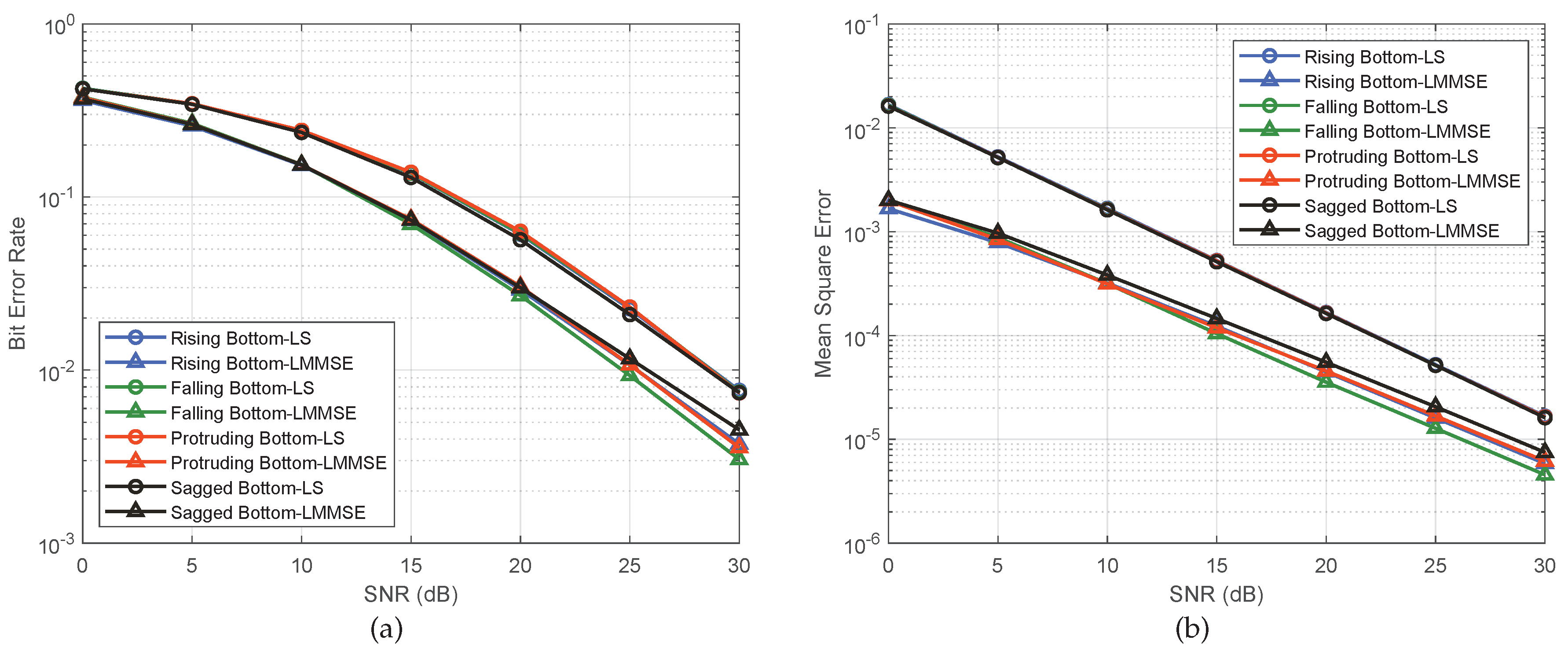
Figure 11 is plotted to compare the BER and MSE performance between the four channels. The BER performance of different channels in LS algorithm is all around 0.0075 when SNR is 30 dB. The value is similar to the worse BER value in Figure 8a, implicating that there may exist a worst-case performance bound of UWA channel estimation through LS algorithm. In addition, the BER performance of different channels in LMMSE algorithm has a few differences. The channel with falling bottom is estimated in the best BER performance while the channel with sagged bottom is estimated in the worst BER performance. The performance of MSE also has similar characteristics to that of BER in LMMSE algorithm, shown in Figure 11b.
4.3. Sea Surface Boundary
In a real ocean environment, the sea surface boundaries are usually not flat. The last simulation is designed to model UWA channels with different sea surface boundaries and analyse the impact on OFDM channel estimation. In this simulation, the receiving depth is fixed at 10 m and UWA channels are modelled in the sea area of scenario A with flat sea bottom boundary, according to the experience of previous simulations. For the sake of high complexity in stochastic channel simulation, LS algorithm is used to estimate UWA channel in this simulation.
First, four UWA channels are modelled with different sea surface boundaries, which are generated by Gauss-Lagrange wave model with measured SWH (1.29 m). Figure 12 shows the eigenrays of different sea surface boundaries. As can be seen from the figures, the stochastic wave boundaries have variable influence on reflection angle, which leads to the number of reflection changes.
Furthermore, Figure 13 shows the normalized CIRs of channels with different sea surface boundaries. In this figure, the effect of sea surface appears as the change of time delay and response amplitude. The CIRs of channels with sea surface 2, sea surface 3, and sea surface 4 are more concentrated than that with sea surface 1. Furthermore, the CIR of channel with sea surface 4 has the maximum amplitude (0.9702).
Figure 14a shows BER performance in different sea surface boundaries. Comparing with the BER performance in UWA channel with flat sea surface boundary channel in Figure 8a, the Gauss-Lagrange waves can improve or deteriorate the BER performance of OFDM channel estimation to some extent. The BER performance of channels with sea surface 1, sea surface 2 and sea surface 3 has a range of deterioration from 1.50 dB to 19.38 dB, while the BER performance of channel with sea surface 4 has an improvement of 10.86 dB.The MSE performance of the four channels has the same value as that in previous simulations, which are illustrated in Figure 14b.
From the figures above, the result of different BER value is mainly caused by the stochastic effect of sea surface on the reflection angle of interfering eigenrays. The main energy of CIRs comes from the blue eigenrays (eigenrays hitting bottom only) that are the same in the four channels. Owing to the stochastic effect of sea surface on the reflection angle of interfering eigenrays which are mainly composed of black eigenrays that stand for the eigenrays hitting both boundaries, the amplitudes and delay of interfering eigenrays are different. In the channel with sea surface 1, the interfering eigenrays have more rebounds than that in the channel with sea surface 4. As a result, the interfering eigenrays in the channel with sea surface 1 have shorter time delay and higher amplitudes, which leads to a worse channel estimation performance.
The result above reveals the stochastic effect of sea surface and explains the reason for the deviation between modelled channels and real channels in [20]. In order to further investigate the statistical effect on OFDM channel estimation, batch of channels with 0.5 m, 1.29 m, and 2 m SWH are modelled and compared in terms of BER performance.
Figure 15a shows the BER curves of channels with different SWH. The blue, green, and red curves represent the BER performance of the modelled channel with 0.5 m, 1.29 m, and 2 m SWH, respectively. For each color, there are 20 curves. When SNR is 30 dB, the worst curves of the three colors have similar BER value with the worst curves in Figure 8a and Figure 11a, which confirms the existence of worst-case performance bound of UWA channel estimation through LS algorithm. Considering the distribution characteristic of curves in different colors, the blue, green, and red curves are mainly concentrated in the high, middle, and low BER performance part of the distribution range, respectively.
Figure 15b shows the quantitative result by plotting the mean channel estimation BER curves for each value of SWH. It is obvious that the mean BER performance of stochastic channels is worse than that of channel with flat sea surface. As the SWH rises, the average performance gradually increases. When SNR is 30 dB, UWA channel with 2 m SWH is 7.95 dB better than that with 0.5 m SWH and 8.06 dB worse than that with flat sea surface. The result is mainly caused by the effect of sea surface and the worst-case performance bound. According to the analysis of Figure 12, Figure 13 and Figure 14, sea surface can affect the time delay and amplitudes of interfering eigenrays, which leads to the variation of estimation performance. As SWH rises, the variation becomes bigger and makes channel estimation more likely to get better or worse performance while the worst-case performance bound limits the performance from getting worse. Consequently, the channels with high SWH can get better average performance of channel estimation. In addition, the possibility of negative effect of sea surface is more than the positive effect, which makes the rough surface channel get worse average performance of channel estimation than the flat surface channel.
5. Conclusions
In this article, we design a comprehensive simulation platform combining UWA channel modelling with OFDM channel estimation. The simulation platform is presented in a GUI and interfaced from various databases, allowing the user to model realistic UWA channels in most areas of the ocean and estimate channels with configurable inputs. Three simulations are conducted based on the simulation platform. Realistic UWA channels in the East China Sea are modelled to study the influence of receiving depth, sea bottom boundary, and sea surface boundary on OFDM channel estimation. The simulations present that different environmental factors have specific effects on rays tracing, which result in the change of time delay and amplitudes, causing the specific effect on the performance of channel estimation. The results show that: (1) The UWA channel with 10 m receiving depth has more concentrated normalized CIR and better channel estimation performance than the other channels with deeper receiving depth. When SNR is 30 dB, the gap of performance reaches around 20 dB in LS algorithm and 30 dB in LMMSE algorithm. (2) The UWA channels with complicated sea bottom boundaries yield poor channel estimation. The BER performance of the channels in LS algorithm is around 0.0075, which is similar to the worse BER value in the first simulation. A worst-case performance bound exists in LS algorithm in which the UWA channels can hardly get worse performance of channel estimation. (3) The sea surface modelled in Gauss-Lagrange waves only affects the interfering eigenrays and has a stochastic effect on the performance of channel estimation. With the increase of SWH, the average performance gradually gets better because of the worst-case performance bound and increasing range of stochastic effect. Though the effect is stochastic, the rough surface channels get worse average performance than the flat one. When SNR is 30 dB, the 2 m SWH channels get 7.95 dB better mean BER performance than the 0.5 m SWH channels and 8.06 dB worse mean BER performance than the flat surface channel in the LS algorithm.
Author Contributions
Conceptualization, X.W. (Xiaoyu Wang) and R.J.; Formal analysis, X.W. (Xiaohua Wang) and Q.C.; Methodology, X.W. (Xiaohua Wang) and X.W. (Xinghua Wang); Resources, R.J. and W.W.; Software, X.W. (Xiaoyu Wang); Writing—original draft, X.W. (Xiaoyu Wang); Writing—review & editing, Q.C. and X.W. (Xinghua Wang).
Funding
This research received no external funding.
Conflicts of Interest
The authors declare no conflict of interest.
References
- Headrick, R.; Freitag, L. Growth of underwater communication technology in the U.S. Navy. IEEE Commun. Mag. 2009, 47, 80–82. [Google Scholar] [CrossRef]
- Baptista, A.; Howe, B.; Freire, J.; Maier, D.; Silva, C. Scientific Exploration in the Era of Ocean Observatories. Comput. Sci. Eng. 2008, 10, 53–58. [Google Scholar] [CrossRef]
- Shin, D.; Na, S.Y.; Kim, J.Y.; Baek, S.J. Fish Robots for Water Pollution Monitoring Using Ubiquitous Sensor Networks with Sonar Localization. In Proceedings of the IEEE 2007 International Conference on Convergence Information Technology (ICCIT 2007), Hydai Hotel Gyeongui, Korea, 21–23 November 2007. [Google Scholar] [CrossRef]
- Dalbro, M.; Eikeland, E.; In’t Veld, A.J.; Gjessing, S.; Lande, T.S.; Riis, H.K.; Søråsen, O. Wireless Sensor Networks for Off-shore Oil and Gas Installations. In Proceedings of the IEEE 2008 Second International Conference on Sensor Technologies and Applications (sensorcomm 2008), Cap Esterel, France, 25–32 August 2008. [Google Scholar] [CrossRef]
- Stojanovic, M.; Preisig, J. Underwater acoustic communication channels: Propagation models and statistical characterization. IEEE Commun. Mag. 2009, 47, 84–89. [Google Scholar] [CrossRef]
- Wang, X.; Ho, P.; Wu, Y. Robust channel estimation and ISI cancellation for OFDM systems with suppressed features. IEEE J. Sel. Areas Commun. 2005, 23, 963–972. [Google Scholar] [CrossRef]
- Mostofi, Y.; Cox, D.C. ICI mitigation for pilot-aided OFDM mobile systems. IEEE Trans. Wirel. Commun. 2005, 4, 765–774. [Google Scholar] [CrossRef]
- John Proakis, M.S. Digital Communications; IRWIN: Boston, MA, USA, 2007. [Google Scholar]
- Etter, P.C. Underwater Acoustic Modeling and Simulation; Spon Press (Tay & Francis Group): Boca Raton, FL, USA, 2013; pp. 351–383. [Google Scholar]
- Zajic, A. Mobile-to-Mobile Wireless Channels; Artech House Books: Norwood, MA, USA, 2013. [Google Scholar]
- Zajic, A.G. Statistical Modeling of MIMO Mobile-to-Mobile Underwater Channels. IEEE Trans. Veh. Technol. 2011, 60, 1337–1351. [Google Scholar] [CrossRef]
- Qarabaqi, P.; Stojanovic, M. Statistical Characterization and Computationally Efficient Modeling of a Class of Underwater Acoustic Communication Channels. IEEE J. Ocean. Eng. 2013, 38, 701–717. [Google Scholar] [CrossRef]
- Naderi, M.; Patzold, M.; Zajic, A.G. A geometry-based channel model for shallow underwater acoustic channels under rough surface and bottom scattering conditions. In Proceedings of the 2014 IEEE Fifth International Conference on Communications and Electronics (ICCE), Danang, Vietnam, 30 July–1 August 2014. [Google Scholar] [CrossRef]
- Radosevic, A.; Proakis, J.G.; Stojanovic, M. Statistical characterization and capacity of shallow water acoustic channels. In Proceedings of the OCEANS 2009-EUROPE, Bremen, Germany, 11–14 May 2009. [Google Scholar] [CrossRef]
- Galvin, R.; Coats, R. A stochastic underwater acoustic channel model. In Proceedings of the OCEANS 96 MTS/IEEE Conference Proceedings, The Coastal Ocean—Prospects for the 21st Century, Fort Lauderdale, FL, USA, 23–26 September 1996. [Google Scholar] [CrossRef]
- Tomasi, B.; Casari, P.; Badia, L.; Zorzi, M. A study of incremental redundancy hybrid ARQ over Markov channel models derived from experimental data. In Proceedings of the Fifth ACM International Workshop on UnderWater Networks—WUWNet’10, Woods Hole, MA, USA, 30 September–1 October 2010. [Google Scholar] [CrossRef]
- Yang, W.B.; Yang, T.C. High-frequency channel characterization for M-ary frequency-shift-keying underwater acoustic communications. J. Acoust. Soc. Am. 2006, 120, 2615–2626. [Google Scholar] [CrossRef]
- Ocean Acoustics Library, Rays. Available online: http://oalib.hlsresearch.com/ (accessed on 12 December 2018).
- Bellhop Gaussian Beam/Finite Element Beam Code. Available online: http://oalib.hlsresearch.com/Rays (accessed on 12 December 2018).
- Tomasi, B.; Zappa, G.; McCoy, K.; Casari, P.; Zorzi, M. Experimental study of the space-time properties of acoustic channels for underwater communications. In Proceedings of the OCEANS’10 IEEE SYDNEY, Sydney, Australia, 24–27 May 2010. [Google Scholar] [CrossRef]
- Jiang, R.; Cao, S.; Xue, C.; Tang, L. Modeling and analyzing of underwater acoustic channels with curvilinear boundaries in shallow ocean. In Proceedings of the 2017 IEEE International Conference on Signal Processing, Communications and Computing (ICSPCC), Xiamen, China, 22–25 October 2017. [Google Scholar] [CrossRef]
- Bahrami, N.; Khamis, N.H.H.; Baharom, A.B. Study of Underwater Channel Estimation Based on Different Node Placement in Shallow Water. IEEE Sens. J. 2016, 16, 1095–1102. [Google Scholar] [CrossRef]
- Bahrami, N.; Khamis, N.H.H.; Baharom, A.; Yahya, A. Underwater Channel Characterization to Design Wireless Sensor Network by Bellhop. Telecommun. Comput. Electron. Control 2016, 14, 110–118. [Google Scholar] [CrossRef]
- Gul, S.; Zaidi, S.S.H.; Khan, R.; Wala, A.B. Underwater acoustic channel modeling using BELLHOP ray tracing method. In Proceedings of the 2017 14th International Bhurban Conference on Applied Sciences and Technology (IBCAST), Islamabad, Pakistan, 10–14 January 2017. [Google Scholar] [CrossRef]
- Nee, R.V. Ofdm for Wireless Multimedia Communications; Artech House Inc.: Norwood, MA, USA, 1999. [Google Scholar]
- Van de Beek, J.J.; Edfors, O.; Sandell, M.; Wilson, S.; Borjesson, P. On channel estimation in OFDM systems. In Proceedings of the 1995 IEEE 45th Vehicular Technology Conference, Countdown to the Wireless Twenty-First Century, Chicago, IL, USA, 25–28 July 1995. [Google Scholar] [CrossRef]
- Sutar, M.B.; Patil, V.S. LS and MMSE estimation with different fading channels for OFDM system. In Proceedings of the 2017 International conference of Electronics, Communication and Aerospace Technology (ICECA), Coimbatore, India, 20–22 April 2017. [Google Scholar] [CrossRef]
- Aida, Z.; Ridha, B. LMMSE channel estimation for block—Pilot insertion in OFDM systems under time varying conditions. In Proceedings of the 2011 11th Mediterranean Microwave Symposium (MMS), Hammamet, Tunisia, 8–10 September 2011. [Google Scholar] [CrossRef]
- Noh, M.; Lee, Y.; Park, H. Low complexity LMMSE channel estimation for OFDM. IEE Proc. Commun. 2006, 153, 645. [Google Scholar] [CrossRef]
- Porter, M.B.; Bucker, H.P. Gaussian beam tracing for computing ocean acoustic fields. J. Acoust. Soc. Am. 1987, 82, 1349–1359. [Google Scholar] [CrossRef]
- Jensen, F.B.; Kuperman, W.A.; Porter, M.B.; Schmidt, H. Computational Ocean Acoustics, AIP Series in Modern Acoustics And Signal Processing; American Institute of Physics: New York, NY, USA, 1994; Volume 80. [Google Scholar]
- Porter, M.B. The Bellhop Manual and User’s Guide: Preliminary Draft; Heat, Light, and Sound Research, Inc.: La Jolla, CA, USA, 2011. [Google Scholar]
- Lindgren, G. Prev—A Wafo module for Analysis of Random Lagrange Waves, Mathematical Statistics; Lund University: Lund, Sweden, 2015. [Google Scholar]
- AVISO+, GRIDDED WIND/WAVE PRODUCTS. Available online: https://www.aviso.altimetry.fr/en/data/products/windwave-products/mswhmwind.html (accessed on 12 December 2018).
- World Ocean Atlas 2013. Available online: https://www.nodc.noaa.gov/OC5/woa13/woa-info.html (accessed on 12 December 2018).
- Wong, G.S.K.; Zhu, S.-M. Speed of sound in seawater as a function of salinity, temperature, and pressure. J. Acoust. Soc. Am. 1995, 97, 1732–1736. [Google Scholar] [CrossRef]
- Google Maps Platform. Available online: https://cloud.google.com/maps-platform/ (accessed on 12 December 2018).
Figure 1.
Block diagram of orthogonal frequency division multiplexing (OFDM) system transceiver.

Figure 2.
The user interface of simulation platform. (a) underwater acoustic (UWA) channel modelling. (b) OFDM channel estimation.
Figure 2.
The user interface of simulation platform. (a) underwater acoustic (UWA) channel modelling. (b) OFDM channel estimation.

Figure 3.
Flow chart of using simulation platform.

Figure 4.
Data flow diagram.

Figure 5.
(a) Geographical location of two scenarios in simulations. (b) sound speed profile (SSP) curve generated from WOA2013.
Figure 5.
(a) Geographical location of two scenarios in simulations. (b) sound speed profile (SSP) curve generated from WOA2013.

Figure 6.
Eigenrays of channel with different receiving depth. The color of lines indicates whether eigenrays hit surface boundary or bottom boundary of the sea. Receiving depth of each figure: (a) 10 m; (b) 30 m; (c) 50 m; (d) 70 m.
Figure 6.
Eigenrays of channel with different receiving depth. The color of lines indicates whether eigenrays hit surface boundary or bottom boundary of the sea. Receiving depth of each figure: (a) 10 m; (b) 30 m; (c) 50 m; (d) 70 m.

Figure 7.
Normalized channel impulse responses (CIRs) of channel with different receiving depth. Receiving depth of each figure: (a) 10 m; (b) 30 m; (c) 50 m; (d) 70 m.
Figure 7.
Normalized channel impulse responses (CIRs) of channel with different receiving depth. Receiving depth of each figure: (a) 10 m; (b) 30 m; (c) 50 m; (d) 70 m.

Figure 8.
(a) bit error rate (BER) performance of channels in different receiving depth, estimated by LS and LMMSE algorithms, respectively. (b) MSE performance of channels in different receiving depth, estimated by LS and LMMSE algorithms, respectively.
Figure 8.
(a) bit error rate (BER) performance of channels in different receiving depth, estimated by LS and LMMSE algorithms, respectively. (b) MSE performance of channels in different receiving depth, estimated by LS and LMMSE algorithms, respectively.

Figure 9.
Eigenrays of channel with different sea bottom boundaries. The color of lines indicates whether eigenrays hit surface boundary or bottom boundary of the sea. Sea bottom boundaries of each figure: (a) rising bottom; (b) falling bottom; (c) protruding bottom; (d) sagged bottom.
Figure 9.
Eigenrays of channel with different sea bottom boundaries. The color of lines indicates whether eigenrays hit surface boundary or bottom boundary of the sea. Sea bottom boundaries of each figure: (a) rising bottom; (b) falling bottom; (c) protruding bottom; (d) sagged bottom.

Figure 10.
Normalized CIRs of channel with different sea bottom boundaries. Sea bottom boundaries of each figure: (a) rising bottom; (b) falling bottom; (c) protruding bottom; (d) sagged bottom.
Figure 10.
Normalized CIRs of channel with different sea bottom boundaries. Sea bottom boundaries of each figure: (a) rising bottom; (b) falling bottom; (c) protruding bottom; (d) sagged bottom.

Figure 11.
(a) BER performance of channels in different sea bottom boundaries, estimated by LS and LMMSE algorithms, respectively. (b) MSE performance of channels in different sea bottom boundaries, estimated by LS and LMMSE algorithms, respectively.
Figure 11.
(a) BER performance of channels in different sea bottom boundaries, estimated by LS and LMMSE algorithms, respectively. (b) MSE performance of channels in different sea bottom boundaries, estimated by LS and LMMSE algorithms, respectively.

Figure 12.
Eigenrays of channel with different sea surface boundaries. The color of lines indicates whether eigenrays hit surface boundary or bottom boundary of the sea. Sea surface boundaries of each figure: (a) Sea Surface 1; (b) Sea Surface 2; (c) Sea Surface 3; (d) Sea Surface 4.
Figure 12.
Eigenrays of channel with different sea surface boundaries. The color of lines indicates whether eigenrays hit surface boundary or bottom boundary of the sea. Sea surface boundaries of each figure: (a) Sea Surface 1; (b) Sea Surface 2; (c) Sea Surface 3; (d) Sea Surface 4.

Figure 13.
Normalized CIRs of channel with different sea surface boundaries in 1.29 m SWH. Sea surface boundaries of each figure: (a) Sea Surface 1; (b) Sea Surface 2; (c) Sea Surface 3; (d) Sea Surface 4.
Figure 13.
Normalized CIRs of channel with different sea surface boundaries in 1.29 m SWH. Sea surface boundaries of each figure: (a) Sea Surface 1; (b) Sea Surface 2; (c) Sea Surface 3; (d) Sea Surface 4.

Figure 14.
(a) BER performance of channels in different sea surfaces boundaries. (b) MSE performance of channels in different sea surfaces boundaries.
Figure 14.
(a) BER performance of channels in different sea surfaces boundaries. (b) MSE performance of channels in different sea surfaces boundaries.

Figure 15.
(a) Distribution of BER curves with difference SWH. There are 20 curves for each SWH value. (b) Mean BER performance of channels in different SWH.
Figure 15.
(a) Distribution of BER curves with difference SWH. There are 20 curves for each SWH value. (b) Mean BER performance of channels in different SWH.


Table 1.
Parameters of simulations.
| Parameter Class | Parameters | Values |
|---|---|---|
| UWA Channel Modelling | Transmitting Depth | 10 m |
| Receiving Depth | 10 m, 30 m, 50 m, 70 m | |
| Significant Wave Heitht | 0 m (flat), 0.5 m, 1.29 m (measured), 2 m | |
| Sea Bottom Boundaries | flat, rising, falling, protruding, sagged | |
| Signal Frequency | 10,000 Hz | |
| Number of Beams | 1000 | |
| OFDM Channel Estimation | Modulation Scheme | 16 QAM |
| Symbol Order | Grey | |
| Algorithm | LS, LMMSE | |
| Number of Carriers | 2048 | |
| Size of FFT | 2048 | |
| Length of Cyclic Prefix | 512 | |
| Pilot Interval | 8 | |
| Number of Symbols per frame | 64 |
© 2019 by the authors. Licensee MDPI, Basel, Switzerland. This article is an open access article distributed under the terms and conditions of the Creative Commons Attribution (CC BY) license (http://creativecommons.org/licenses/by/4.0/).
Share and Cite
MDPI and ACS Style
Wang, X.; Wang, X.; Jiang, R.; Wang, W.; Chen, Q.; Wang, X. Channel Modelling and Estimation for Shallow Underwater Acoustic OFDM Communication via Simulation Platform. Appl. Sci. 2019, 9, 447. https://doi.org/10.3390/app9030447
AMA Style
Wang X, Wang X, Jiang R, Wang W, Chen Q, Wang X. Channel Modelling and Estimation for Shallow Underwater Acoustic OFDM Communication via Simulation Platform. Applied Sciences. 2019; 9(3):447. https://doi.org/10.3390/app9030447
Chicago/Turabian StyleWang, Xiaoyu, Xiaohua Wang, Rongkun Jiang, Weijiang Wang, Qu Chen, and Xinghua Wang. 2019. "Channel Modelling and Estimation for Shallow Underwater Acoustic OFDM Communication via Simulation Platform" Applied Sciences 9, no. 3: 447. https://doi.org/10.3390/app9030447
Note that from the first issue of 2016, this journal uses article numbers instead of page numbers. See further details here.