Detection of Pneumatic Conveying by Acoustic Emissions


School of energy power and mechanical engineering, North China Electric Power University, Beijing 102206, China
*
Author to whom correspondence should be addressed.
Appl. Sci. 2019, 9(3), 501; https://doi.org/10.3390/app9030501
Submission received: 17 December 2018
/
Revised: 25 January 2019
/
Accepted: 29 January 2019
/
Published: 1 February 2019
(This article belongs to the Special Issue State of the Art of Acoustic Emissions Applications)
Abstract
:Featured Application
Measurement of the pneumatic conveying parameters.
Abstract
The acoustic emission (AE) method is used in certain industries for the measurement of pneumatic conveying. Instead of the non-intrusive sensors, the comparison of two different intrusive probes in pneumatic conveying is presented in this work, and the AE signals generated by the flow for different particle flow rates and particle sizes were studied. Comparing the distribution of root mean square (RMS) values indicates that the AE signal acquired by a wire mesh probe was more reliable than that from a T-type probe. Limited intrinsic mode functions (IMFs) were extracted from the raw signals by the ensemble empirical mode decomposition (EEMD) algorithm. The characteristics of these signals were analyzed in both the time and frequency domains, and the energies of different IMFs were used to predict the particle mass flow rates, demonstrating a relative error under 10% achieved by the proposed monitoring system. Additionally, the mean squared error contribution fraction, instead of the energy fraction, can predict the particle size.
1. Introduction
Pneumatic conveying is widespread in the power, pharmaceutical, metallurgy, food, and various other industrial processes [1]. The capability of online management and measurement of pneumatic conveying is of great significance for monitoring and control of industrial processes. Considering the coal-fired power plant industry as an example, the mass flow rate and particle size of pulverized coal will directly affect combustion inside of the boiler and the carbon content of the resulting ash, significantly impacting operation efficiency and plant economy. Determining pneumatic conveying parameters, including particle size, particle mass flow rate, flow velocity, and humidity, is complicated, and with current technology, it is challenging to establish an accurate model for these conveying characteristics.
Over the course of many years, researchers have studied and developed a variety of pneumatic conveying measurement methods. Each method has certain advantages over a specific range, but also possesses notable drawbacks. Among these numerous measurement methods, the most commercially promising techniques include ultrasonic [2,3], optical [4,5], electrostatic [6,7], and capacitance [8] approaches, among others. The ultrasonic method is susceptible to temperature and is regarded as difficult to install. The optical method is mainly subject to the pollution of the sampling window. The electrostatic and capacitive method belongs to the electrical category, however, it is hard for the electrostatic sensor to be electrically shielded from the rest of the environment. The capacitance sensor lacks sufficient sensitivity for dilute flows that contains moisture. During the pneumatic conveying process, particle-particle interaction and particle-wall interaction produce particular acoustic signals, which can be detected by acoustic emission (AE) sensors. Since pneumatic conveying generates these signals, they reveal important characteristics about the conveying process. As an added benefit, acoustic emission measurements are simpler and more convenient for this application.
Some researchers investigated the monitoring of particle size by using acoustic emissions method. Leach and Rubin [9] originally introduced three important cases to illustrate the principles of the method. Nevertheless, further application of signal processing techniques on the acoustic emission signal had not been performed. Alessandro et al. [10] applied the approach to research the relationship between AE signal and particle size distribution for limited operating conditions. To this end, they developed a three-step data processing procedure, using wavelet packet decomposition to extract useful features and multivariate data analysis to decrease feature numbers used as the input of the neural network. This led to the development of a neural network to realize particle sizing. For the wavelet packet decomposition process, however, it is necessary to apply multiple adjustments. Uher and Benes [11] experimentally validated the Hertz contact theory in the measurement of particle size distribution, while their experimental results are distinct to practical industrial processes. As a consequence, a more accurate theory is necessary to establish and predict the process. Hu [12] developed an AE-based online particle sizing instrument employing the Hertz theory of contact, and the experimental results were highly consistent with theoretical expectations under limited conditions. However, for increasing solid mass flow rate, the sizing results deviated significantly due to their theoretical assumptions. Hansuld and Briens et al. [13] used the audio AE signals to monitor particle size in pharmaceutical manufacturing. The investigation demonstrated a predictive relationship between the total power spectral density and wet granule size in a 12 L beaker, with the result corresponding to dry sphere measurement. Guo [14] used audio AE signals to monitor particle size in pneumatic conveying, and after decomposition by wavelet analysis, the energy fractions of different components could predict particle size through a neural network. The result showed that relative error was within 23% when experimental particle sizes (e.g. 75/90/110/150/200 μm in the research) were in certain ranges. Additionally, the higher error range indicated that the signal processing should be improved. Among the scientific research mentioned above, only a little portion of relative researches have denoised the raw signal to extract effective signals to develop the relationship between the particle size and the AE signal. Moreover, the acoustic emission signal propagation has not been considered. The propagation process is rapid in the metal pipe. In the relative references mentioned above, the total signal introduced into the sensors is a complex mixture of signals generated by the whole system, making it difficult to detect local characteristics of the particle size.
Some researchers have applied the acoustic emission to the research on particle mass flow rate monitoring in the multiphase flow. Cao [15] decomposed the AE signal by utilizing the seven scales wavelet decomposition method and proposed a model of particle mass flow rate to explore the quantitative relationship between the AE energy, superficial gas velocity and particle mass flow rate. The model is under strict assumption of low speed flow conditions and uniform particle distribution. Nevertheless, particle size distribution was described by the Rosin-Rammler distribution instead of uniform particle distribution. It means that the model developed by Cao was useful in limited situation. Wei [16] developed a regression model between AE energy and particle mass flow rate by using the wavelet packet decomposition and partial least square method. Chen [17] developed an acoustic emission monitoring system to detect the sand mass flow rate and some other parameters. The relationship between the sand mass flow rate and power spectrum amplitude is linearity. His research focused on liquid-solid phases systems instead of pneumatic conveying. Wang [18] studied the relationship of the signal frequency, area of the power spectrum estimation and solid particle size and mass flow rate. The combination of AE signal and power spectrum estimation to detect parameters of pneumatic conveying is feasible and effective. However, the effects of multiple impacts of the same particle were ignored. Through the literature mentioned above, it is apparent that the researchers did not consider the mixture of the signal problem adequately. Involving in the signal processing, the wavelet packet decomposition is used widely. However, the selection of wavelet function and decomposition level is a complex process, which needs manual selection in many situations.
In this paper, acoustic emission signals collected by different probes, subjected to different particle mass flow rates with different particle sizes, were studied. Compared with the wavelet packet decomposition, the ensemble empirical mode decomposition (EEMD) is a more self-adaptive algorithm. The ensemble empirical mode decomposition method was used to decompose the signal, and the effective signal is extracted to establish a specifying relationship between AE signal and mass flow rate, and the relationship of the signal and particle size is built as well.
2. Theoretical Model
Solid particle collisions with the probe generate transient elastic stress waves that propagate away from the point of impact. These waves can be detected by a piezoelectric transducer located a certain distance from the collision site.
According to the Hertz contact theory, the impact frequency relates to the duration of the collision. Hou [19] deduced the frequency of the resulting acoustic signal, assuming that the particle is spherical and that the impact is a completely elastic collision. Accordingly, the frequency can be approximated by:
where is the elastic modulus parameter, and E and σ are the Young’s modulus and the Poisson ratio, respectively; subscripts 1 and 2 refer to the material of the particle’s bulk and its surface, respectively; , , and represent the particle’s density, radius, and approach velocity, respectively. With a certain particle velocity and known material properties, the particle size can be related to the signal frequency, and the particle size distribution can be described by the Rosin-Rammler function. From the equation, it is obvious that the larger the particle size, the smaller the corresponding frequency. Therefore, when the particles in pneumatic conveying collide with the probe or the tube wall, there will be different resulting frequency distributions due to different particle sizes.
Based on the research of Cody [20], He [21] deduced the acoustic energy driven by contact between the particle and wall. The energy can be approximately by:
where η is the transformation efficiency from collision pressure to acoustic pressure; t is the time interval; m is the mass of the particle; and is the particle concentration dispersed within the air volume. and represent the considered interaction area where dispersed particles collide with the wall and the percentage of particles impacting it at an angle of , respectively.
In a real system, the AE signal traveling from sensor to the computer is dependent not only upon this theoretical analysis, but also upon wave propagation effects and the system’s response to surface vibrations. The complete AE signal can be expressed as [22]:
where V(t) represents the measured AE voltage signal, and S(t), G(t), and R(t) are the original acoustic signal, wave propagation function, and the system response, respectively, where the symbol * denotes convolution. The wave propagation medium and the system response function are non-linear and time variant; therefore, it is difficult to develop a direct relationship between the AE signal and pneumatic conveying without signal processing.
3. Ensemble Empirical Mode Decomposition
With the development of modern digital signal processing technology, signal analysis has become an important tool for the study of pneumatic conveying characteristics. Huang et al. [23] proposed an empirical mode decomposition (EMD) method, which is based on the step-wise decomposition of the non-linear non-stationary signal itself. As mentioned above, in real world monitoring of pneumatic conveying, particle size is uncertain, which possess a challenge when defining an effective frequency range. Thus, the EEMD algorithm is suitable for signal decomposition since it utilizes the raw signal, and the EMD method has good adaptability. Each order of the intrinsic mode function (IMF) should satisfy the following two conditions:
- In the entire data sequence, the number of extreme points and the number of zero-crossings should be equal or differ at most by one;
- The mean value of the envelopes determined by the local maxima and local minima at any given data point should be zero.
However, the EMD method can misrepresent the envelope due to the addition of the boundary value, and the local fluctuation can result in mode confusion. Considering these EMD disadvantages, Wu [24] proposed an improvement to the ensemble empirical mode decomposition method, adding a Gaussian-white-noise background to the signal. After several decompositions, the additional noise is eliminated and only the signal remains. The EEMD algorithm decomposition steps are as follows:
- Add white noise to the raw data x(t):where nm(t) is the white noise, and X(t) represents the data (with noise) for the mth trial.
- Decompose the noise-added data X(t) into several IMFs (total number I);
- Repeat steps (1) and (2) several times, each time adding independent random white noise, until the trial number reaches a pre-determined value, m = M, M is the number of trials;
- Calculate the ensemble mean of the M trials for each IMF:
- Finally, decompose the raw data into several IMFs: and a residual component r:
The accuracy of the EEMD method depends on both the chosen amplitude for the added white noise and the number of specified trials. A small amplitude for the added noise will have no influence on the raw signals, whereas a high amplitude will mask the raw signal.
The number of Gaussian white noise to the EEMD obeys the statistical law [25]:
where is the amplitude of the white noise. Generally, the value of is 0.2, and the value of M is 100. In order to ensure that the algorithm converges quickly and results in efficient detection, should not be too small.
Finally, the raw signal x(t) can be decomposed as follows:
4. Experimental System
This section describes the materials required to apply this methodology experimentally, including test materials, a laboratory-scale pneumatic conveying system, and a data acquisition system.
4.1. Test Materials and System
4.1.1. Test Materials
For health and safety considerations, dry glass beads with a density of 2500 kg/m³ were selected as the test material. Baking the glass beads in an electric oven at 100 °C for about 4 h ensured that the beads were dry, which was necessary to reduce the humidity effect on the generated AE signals. Furthermore, drying prevented aggregation to stabilize the size of the glass beads. As a preliminary trial, four particle sizes were chosen, 550 μm, 250 μm, 180 μm, and 150 μm.
4.1.2. System Set-Up
A laboratory-scale flow-loop pneumatic conveying system was developed. Figure 1 shows the system schematic, consisting of several sections of stainless steel pipe or plexiglas pipe.
4.1.3. Particle Feeding System
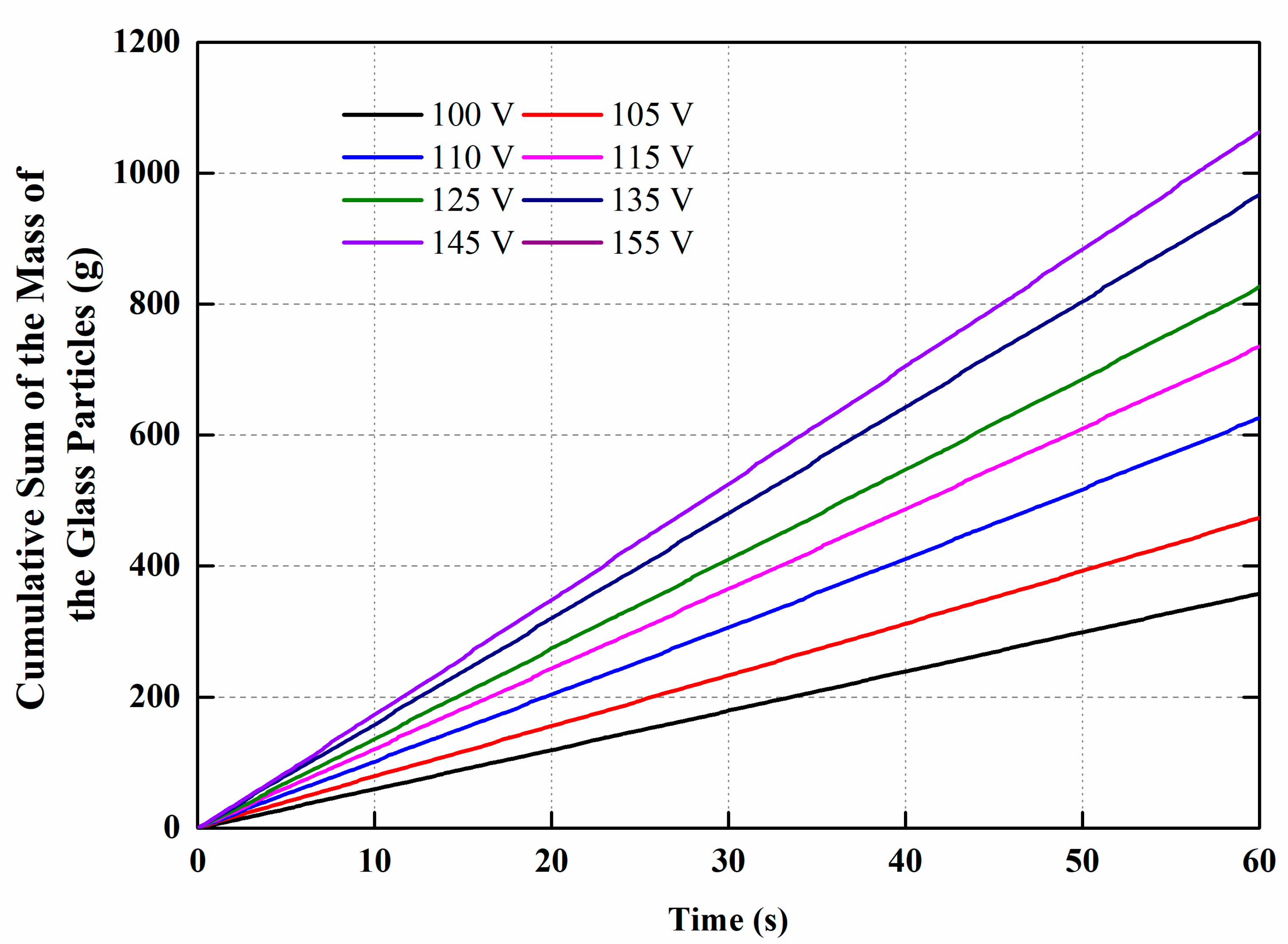
The feeding system consists of two parts: The first is the vibrating feeder, adjusted by a voltage control, and the second part is a hopper above the vibrating feeder. The two components are installed at fixed position to make sure the feeding rate remains constant at a certain voltage. Before the experiments, tests were carried out to investigate the consistency and calibration of the particle flow rates; the results under different control voltage, presented in Figure 2, show that the particle mass flow rates from the vibrating feeder are relatively consistent over a 1 min span.
4.1.4. Piping and Air Conveying System
The piping system was constructed using standard steel pipe with a 50 mm nominal bore, and the horizontal pipes were divided into four parts. The first section is a T-type tee structure that connects the vertical branch with the feeder as the solid inlet; one side is the air inlet, and the other connects to the second section by a flange. The second segment is a plexiglas pipe 1700 mm in length, which functions as a visual monitor to ensure that the particles do not accumulate at the bottom of the pipe. Additionally, there are two holes in the pipe wall for installation of the pitot tube flowmeter and the T-type probe. The Plexiglas pipe then connects with the third section by another flange. There is a special structure in this connection that installs the mesh probe between the two sides of the flange. The third part is a stainless steel pipe (1200 mm in length) that connects with the filter section through a hose, and the filter section connects with the draft fan by a hose as well. The draft fan is manufactured by the Beijing Draft Fan Corporation, Beijing, China, 2014.
Together with the particle feeding system, these instruments allow for independent adjustment of both the bead mass flow rates and concentration
4.2. Data Acquisition System
The measurement and data acquisition (DAQ) system comprises two SR 150M AE sensors (Soundwel Technology Co., Ltd., Beijing, China, 2010) with a 60 kHz–400 kHz bandwidth, two preamplifiers (Soundwel Technology Co., Ltd., Beijing, China, 2010) with 20/40/60 dB adjustable gain, a high-speed DAQ board (four channels, Soundwel Technology Co., Ltd., Beijing, China, 2010), and an industrial control computer.
4.3. Experimental Programs
This research briefly covers three main investigations:
- The effect of different probe types on AE generation;
- The relationship between particle mass flow rate and the AE signal;
- The relationship between particle size and the AE signal.
In all of these experiments, the flow velocity was measured by a pitot tube flowmeter inserted into the piping system. The sampling frequency is 1 MHz and the number of data points for the AE signal is 16,384, with a corresponding sampling time of 16.384 ms. To reduce the influence of the air velocity on the generated AE signals, the flow velocity was set at 21 m/s, as a constant parameter. The particle feeding rates were varied from 6 g/s to 16 g/s with an increment of 2 g/s, and the volumetric particle concentrations for pneumatic conveying at different feeding rates are summarized in Table 1. Each test condition was repeated four times, corresponding to 200 AE samples.
5. Results and Discussion
This section presents and discusses the data acquired by the AE signal acquisition system for the experimental parameters mentioned above.
5.1. Effect of Different Signal Acquisition Methods
To realize an on-line measurement system, data processing time should be short. While the experiments were conducted for fixed conditions, the movement of particles was still disordered. Therefore, the obtained data should be representative of smaller data volumes, as required by a real-time system. Two different probe types were compared. The first one was of the T-type, shown in Figure 3, and the second was the wire-mesh type (Figure 4). When the T-type probe was installed in the system, since the sensitive area is concentrated, only part of the particles would have contact with the T-type probe. Together with the uncertainty of the flow type, the uncertainty of particle impact would increase and unpredictable. The wire-mesh probe does not pose this same challenge. Without increasing the occupation of the cross-sectional area, the wire mesh covers the entire cross-sectional area, while not significantly affecting the pipe’s cross-sectional volume. Thus, the wire-mesh probe can be effectively increasing the number of particle impacts.
Figure 5 presents typical raw AE signals acquired simultaneously by two AE sensors attached on both the T-type and wire-mesh probes. This signal corresponds to a particle mass flow rate of 16 g/s and a particle size of 550 μm. The peak amplitude of the AE signal obtained by the T-type probe is larger than that recorded by the wire-mesh probe. Figure 6 presents the samples retrieved from the raw AE signals, for both probes, and each graph column was collected at the same time. All data in Figure. 6 were extracted randomly from the entire raw signal. One can see that the signals for the T-type fluctuate more than those from the wire-mesh probe. Figure 7a shows the root mean square (RMS) of AE signal for the two probe types. Even though the signal peak-amplitude for the T-type probe is higher, the RMS value for the wire-mesh probe is slightly greater than for the T-type probe. Figure 7b shows that the relative error for the wire-mesh probe deviates less from the zero line, which means that the randomly selected signals acquired by the wire-mesh probe are more representative of the sample. Therefore, it can be concluded that the AE signal is more stable and representative for the wire-mesh probe than for the T-type probe. Figure 8 plots the RMS average values (for all four repeated tests) of the AE signals with respect to particle mass flow rates.
It is worth noting that as mentioned, the AE signal RMS obtained by the wire-mesh probe is higher than for the T-type probe, and this value gap increases with a growing particle mass flow rate.
5.2. Relationship Between Particle Mass Flow Rate/Size and The Ae Signal
In this section, the influences of particle mass flow rate and size were investigated. As discussed, the AE signals obtained by the wire-mesh probe are more reliable and representative than the signals obtained by the T-type probe. Therefore, the data used in this section results from the wire-mesh probe sensor.
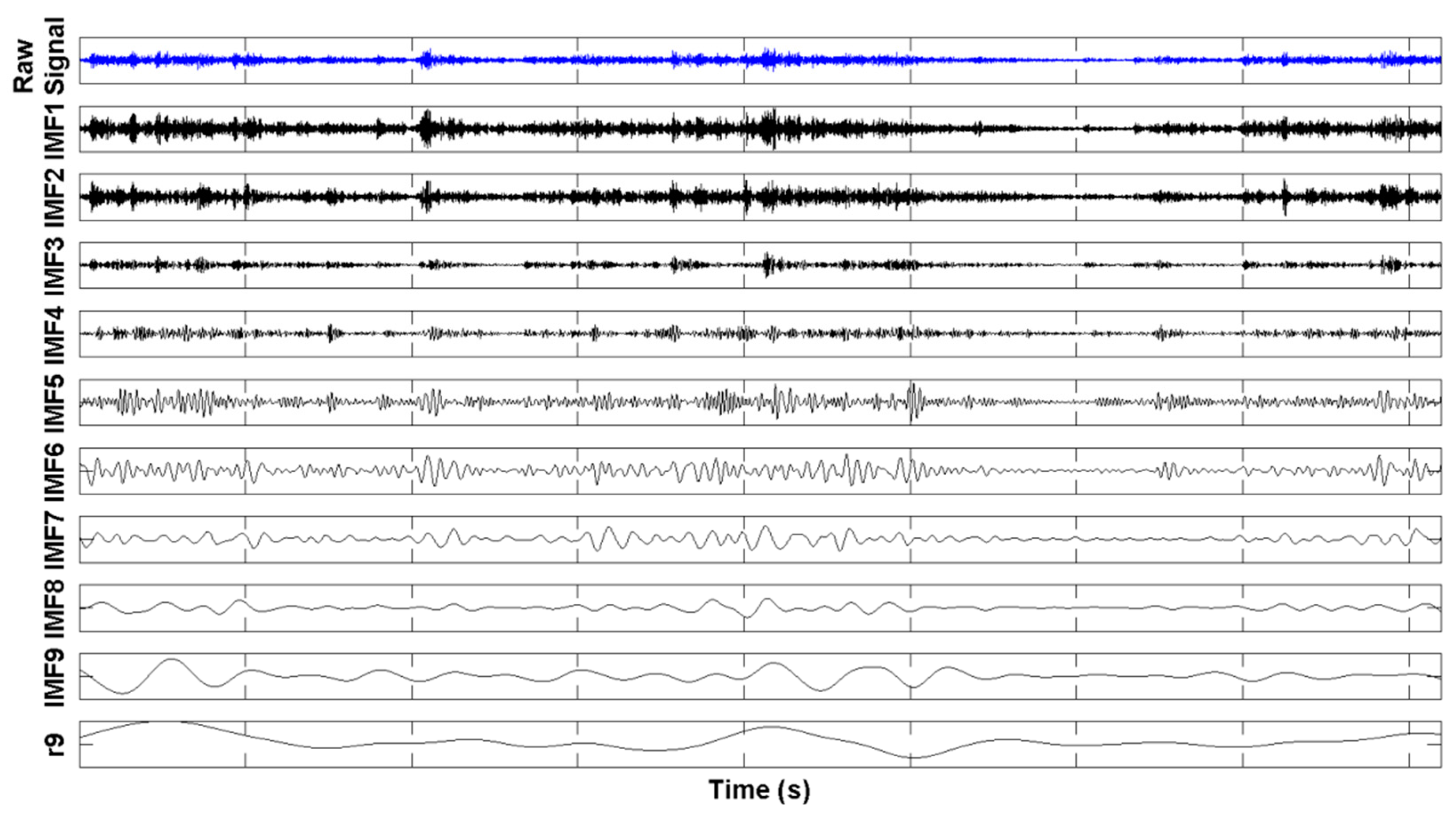
First, the AE signals under a particle mass flow rate of 14 g/s and a particle size of 150 μm were analyzed. It can be seen from Figure 9 that nine IMF components, together with a residual r9, were generated from the AE signal. In the time domain, the amplitude of all IMF components decreases by several orders of magnitude from the highest value in IMF1 to the lowest in IMF9. In the frequency domain, the same trend was observed, displayed in Figure 10, i.e., IMF1 has the highest instantaneous frequency and IMF9 has the lowest.
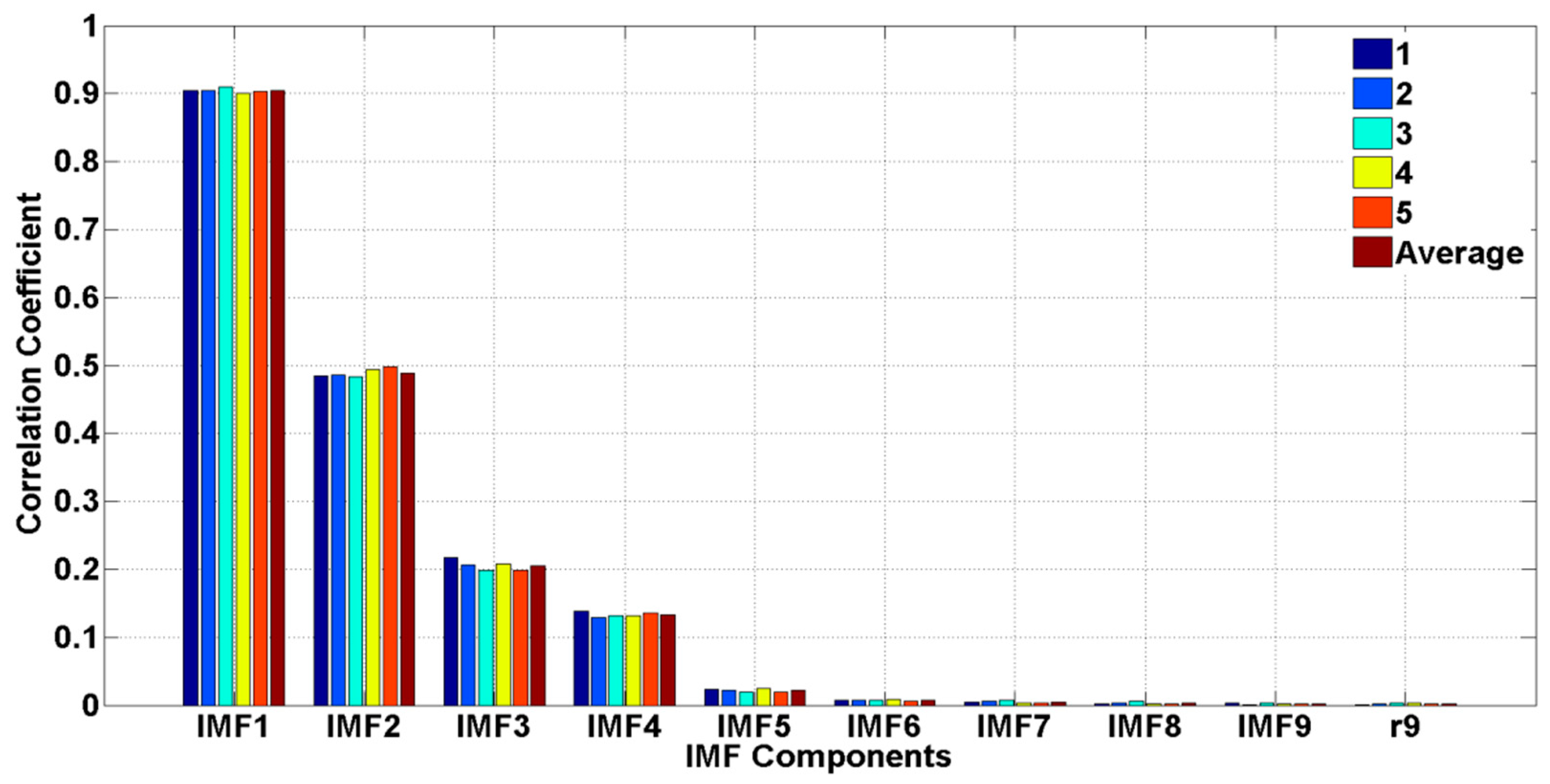
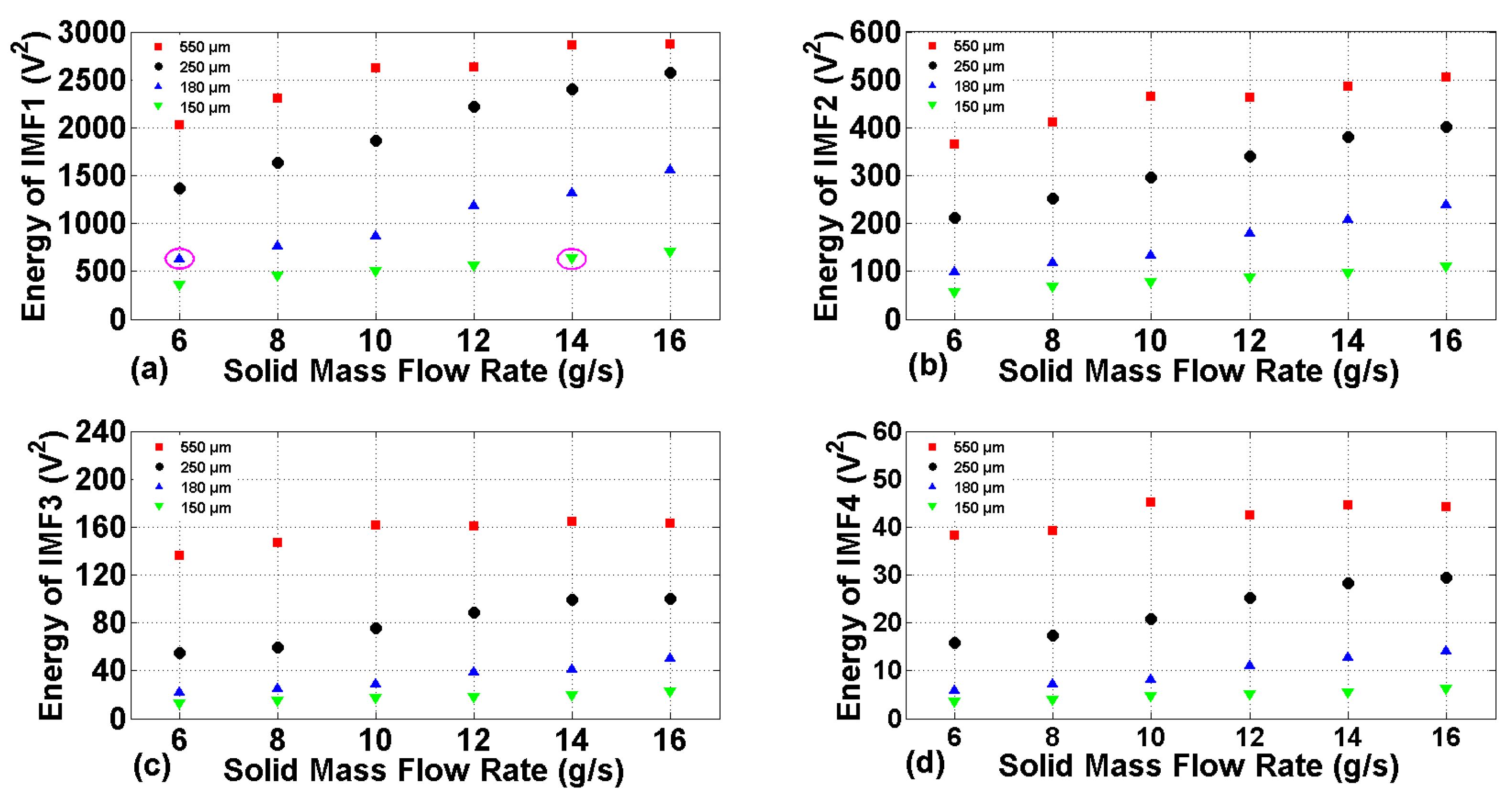
To reduce the influence of random error, five random AE signal samples were selected and decomposed. In order to select useful features from the IMF components, the correlation coefficients between different IMF components and the raw AE signal were computed, given in Figure 11 showing that the correlation coefficients for IMF1 to IMF4 are above 0.1. This means that all these four components have the potential to represent the raw sample signals to show a relationship between the AE signal and pneumatic conveying parameters. The relationship between the energies magnitudes for different IMFs, corresponding to the wire-mesh probe and the particle mass flow rate, is presented in Figure 12.
It can be concluded that given the same particle size, with an increasing particle mass flow rate, the energy of IMFs will gradually increase. This can be explained, under certain conditions, since the increase in particle mass flow rate boosts the number of effective interactions, it causes an energy increase in the IMFs. Additionally, under the same airflow and particle mass flow rate, an increase in particle size results in rising IMF energy as well. This phenomenon is due to the high kinetic energy of single particles.
To analyze the relationship between the features and particle flow rate, a linear-fitted line for the energies of the IMFs under given particle size is computed, and a parameter termed as the average relative deviation from linearity, δ, is introduced and defined as:
where is the experimental energy under different mass flow rates; is the corresponding value for the fitted line, given the same condition represented by ; and M is the number of particle mass flow rate conditions. δ can illustrate the performance of the line fitting, and Figure 13 shows the average relative deviation for different IMF components. Apparently, all δ-values are under 0.1 (10%), meaning that they are all acceptable for an industrial process. Considering the four particle sizes, IMF3 or IMF4 may be best suited to develop the relationship for particle mass flow rate measurement in industrial processes.
After determining a fitting process, additional experimental conditions sought to validate the approach, and the results are presented in Table 2. After analysis by the EEMD method, all of the results were compared with the described fitting function, and the resulting relative deviations are displayed in Table 3. One can note that all of the relative deviations are under 10%. In view of these additional data points, it is clear that the energies for IMF3 and IMF4 have the best linear relationship with particle mass flow rates for different particle sizes, which is useful in characterizing flow rate change.
In Figure 12a, there are two magenta ovals to specify two data points that, while representing different conditions, nearly share the same energy value. To consider this further, Table 4 presents the IMF energies for the two different conditions. The first row represents a particle mass flow rate of 6 g/s and a particle size of 180 μm; the second row corresponds to 14 g/s and 150 μm, respectively. This side-by-side comparison validates the value similarity between the two IMF components, which shows a case where distinguishing the two could result in an incorrect judgment. Therefore, at least two parameters are required to avoid incorrect judgment.
In this paper, the mean-squared error contribution fraction (MSECF) for different IMFs is defined as:
which indicates the importance of the IMF components to the raw AE signal. N is the sampling number (set as N = 16384); is the mean-squared error; and m is the number of the IMF component.
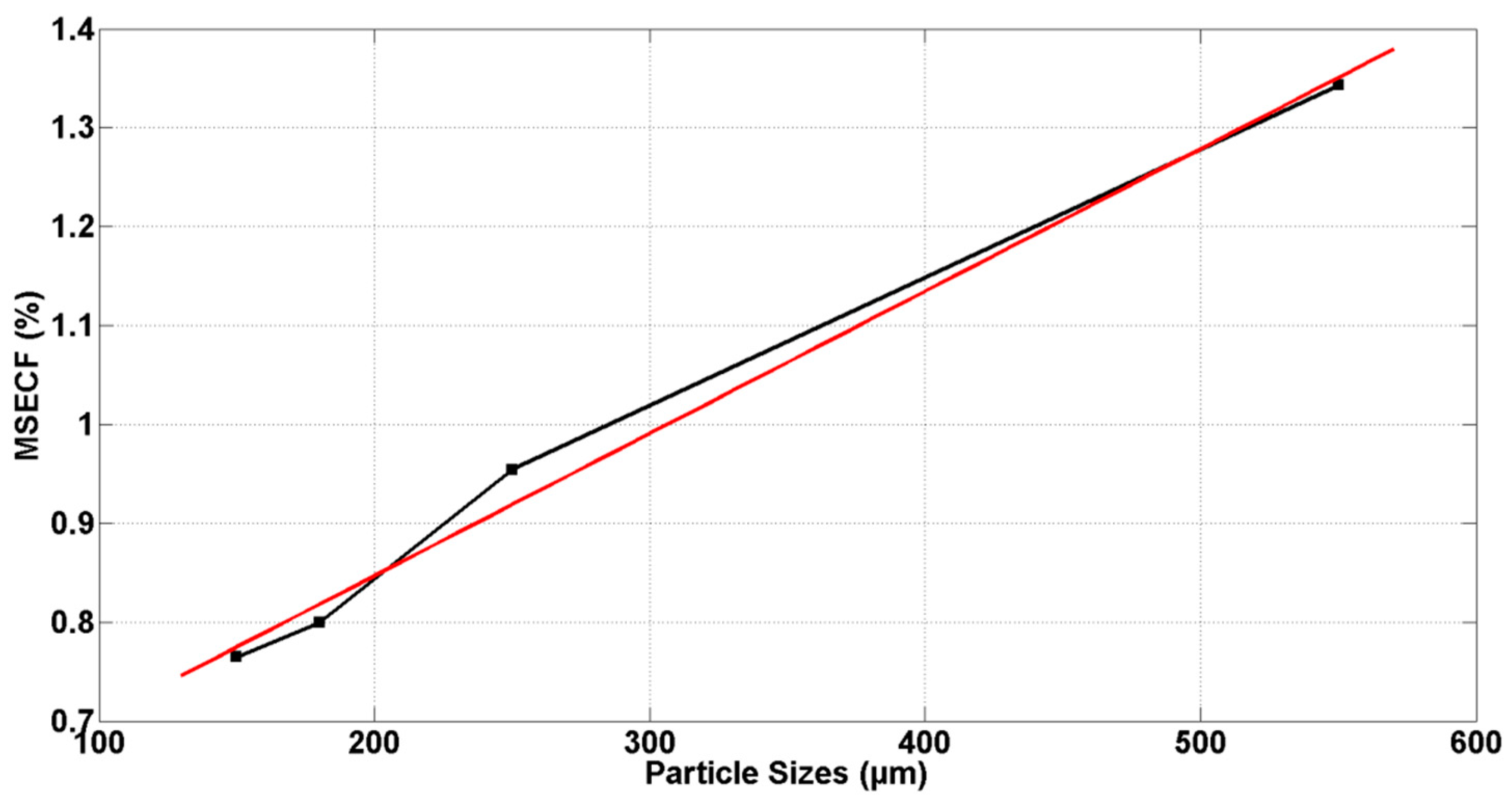
Figure 14 presents the MSECF for different IMF components. As the particle size increases, according to the formula 1, the dominant frequency of the AE signal gradually decrease, which result in a gradual decrease in the MSECF of the high frequency components. This can explain why the MSECF of the IMF1 would have a reversely performance compared with other IMF components, and the curves for IMF4 indicate the four particle sizes clearly. Therefore, the MSECF may perform better when distinguishing particle size. The linear fit for the average MSECF respective of particle size is presented in Figure 15, with the fitting equation:
In this fitting function, y is the MSECF value, and x represent the particle flow rate. The adjusted R-Squared of the curve is 0.98745, which indicates a good fit.
6. Conclusions
This paper develops two intrusive probes to collect the AE signals in pneumatic conveying, compares the AE signals characteristics of the two probes and analyze the relationship between the signals and particle flow rate or particle size. The conclusions are as follows:
- Comparison of the RMS values of AE signals illustrates that the acoustic emission signal acquired by a wire mesh is more reliable than the T-type probe.
- After the signals decomposed by the EEMD algorithm, the IMF1 to IMF4 have the potential to represent the raw sample signals to show a relationship between the AE signal and pneumatic conveying parameters.
- By comparing the average relative deviation, it is obvious that the energies of the IMF3 or IMF4 can be used to develop a linear relationship with particle flow rate.
- Instead of the energies of the IMF components, the MSECF of IMF4 have a good performance to distinguish particle size.
Author Contributions
Conceptualization, L.A. and W.L.; Methodology, W.L. and G.S.; Software, W.L. and Y.J.; Validation, W.L. and Y.J.; Formal Analysis, W.L. and Y.J.; Investigation, W.L. and S.Z.; Resources, S.Z.; Data Curation, W.L. and Y.J.; Writing-Original Draft Preparation, W.L. and Y.J.; Writing-Review & Editing, G.S.; Visualization, L.A. and G.S.; Supervision, L.A. and G.S.; Project Administration, G.S.; Funding Acquisition, G.S. and W.L.
Funding
This research was funded by the Fundamental Research Funds for the Central Universities (grant number 2015XS83 and 2017ZZD001) and National Key R&D Program of China (2018YFB0604305-05).
Conflicts of Interest
The authors declare no conflict of interest.
References
- David, M. A review of pneumatic conveying systems. In Pneumatic Conveying Design Guide, 3rd ed.; Elsevier Ltd.: Chatswood, NSW, Australia, 2016; pp. 59–80. [Google Scholar]
- Millen, M.J.; Sowerby, B.D.; Coghill, P.J.; Tickner, J.R.; Kingsley, R.; Grima, C. Plant tests of an on-line multiple-pipe pulverised coal mass flow measuring system. Flow Meas. Instrum. 2000, 11, 153–158. [Google Scholar] [CrossRef]
- Allashi, R.S.; Challis, R.E. Ultrasonic particle sizing in aqueous suspensions of solid particles of unknown density. J. Acoust. Soc. Am. 2015, 138, 1023–1029. [Google Scholar] [CrossRef] [PubMed] [Green Version]
- Keep, T.; Noble, S.D. Optical flow profiling method for visualization and evaluation of flow disturbances in agricultural pneumatic conveyance systems. Comput. Electron. Agric. 2015, 118, 159–166. [Google Scholar] [CrossRef]
- Wang, W.; Guan, Q.; Wu, Y.; Yang, H.; Zhang, J.; Lu, J. Experimental study on the solid velocity in horizontal dilute phase pneumatic conveying of fine powders. Powder Technol. 2011, 212, 403–409. [Google Scholar]
- Shao, J.; Krabicka, J.; Yan, Y. Velocity measurement of pneumatically conveyed particles using intrusive electrostatic sensors. IEEE Trans. Instrum. Meas. 2010, 59, 1477–1484. [Google Scholar] [CrossRef]
- Wang, C.; Zhang, J.Y.; Zheng, W.; Gao, W.; Jia, L. Signal decoupling and analysis from inner flush-mounted electrostatic sensor for detecting pneumatic conveying particles. Powder Technol. 2017, 305, 197–205. [Google Scholar] [CrossRef]
- Zhou, W.T.; Jiang, Y.; Liu, S.; Zhao, Q.; Long, T.; Li, Z. Detection of gas-solid two-phase flow based on CFD and capacitance method. Appl. Sci. 2018, 8, 1367. [Google Scholar] [CrossRef]
- Leach, M.F.; Rubin, G.A.; Williams, J.C. Particle size determination from acoustic emissions. Powder Technol. 1977, 16, 153–158. [Google Scholar] [CrossRef]
- Alessandro, B.; Cristalli, C.; Morlacchi, R.; Pomponi, E. Acoustic emissions for particle sizing of powders through signal processing techniques. Mech. Syst. Signal Process. 2011, 25, 901–916. [Google Scholar]
- Miroslav, U.; Peter, B. Measurement of particle size distribution by the use of acoustic emission method. In Proceedings of the Instrumentation and Measurement Technology Conference, Graz, Australia, 13–16 May 2012; pp. 1194–1198. [Google Scholar]
- Hu, Y.H.; Qian, X.C.; Huang, X.B. Online continuous measurement of the size distribution of pneumatically conveyed particles by acoustic emission methods. Flow Meas. Instrum. 2014, 40, 163–168. [Google Scholar] [CrossRef]
- Hansuld, E.M.; Briens, L.; Mccann, J.A.; Sayani, A. Audible acoustics in high-shear wet granulation: Application of frequency filtering. Int. J. Pharm. 2009, 378, 37–44. [Google Scholar] [CrossRef] [PubMed]
- Guo, M.; Yan, Y.; Hu, Y.H.; Sun, D.; Qian, X.; Han, X. On-line measurement of the size distribution of particles in a gas–solid two-phase flow through acoustic sensing and advanced signal analysis. Flow Meas. Instrum. 2014, 40, 169–177. [Google Scholar] [CrossRef]
- Cao, Y.J.; Wang, J.D.; Yang, Y.R. Multi-scale analysis of acoustic emissions and measurement of particle mass flowrate in pipeline. Chin. J. Chem. Eng. 2007, 58, 1404–1410. [Google Scholar]
- Wei, G.Y.; Zhou, Y.; Liao, Z.; Wang, J.; Yang, Y. Detection of particle mass flowrate in high-speed fluidization based on acoustic emission technology. Acta Pet. Sin. 2011, 27, 773–779. [Google Scholar]
- Chen, C. Research on Flow Detection of Oil-Sand Phases Based on Acoustic Emission Technology. Master’s Thesis, College of Petroleum Engineering, China University of Petroleum, Shandong, China, 2013. [Google Scholar]
- Wang, Z.C.; Yuan, X.J.; Wang, Y.M.; Li, H.G. Gas-solid two-phase mass flow rate and particle size measurement based on acoustic emission. Instrum. Tech. Sens. 2017, 7, 93–96. [Google Scholar]
- Hou, L.X. Study on Acoustic Emission Measurement and Multi-Scale Structure of Fluidized Bed Polymerizer. Ph.D. Dissertation, Department of Chemical Engineering, Zhejiang University, Zhejiang, China, 2005. [Google Scholar]
- Cody, G.D.; Bellows, R.J.; Goldfarb, D.J. A novel non-intrusive probe of particle motion and gas generation in the feed injection zone of the feed riser of a fluidized bed catalytic cracking unit. Powder Technol. 2000, 110, 128–142. [Google Scholar] [CrossRef]
- He, L.; Zhou, Y.; Huang, Z.; Lungu, M.; Yang, Y. Acoustic analysis of particle–wall interaction and detection of particle mass flow rate in vertical pneumatic conveying. Ind. Eng. Chem. Res. 2014, 53, 9938–9948. [Google Scholar] [CrossRef]
- Buttle, D.J.; Scruby, C.B. Characterization of particle impact by quantitative acoustic emission. Wear 1990, 137, 63–97. [Google Scholar] [CrossRef]
- Huang, N.E.; Shen, Z.; Long, S.R.; Wu, M.C.; Shih, H.H.; Zheng, Q.; Yen, N.C.; Tung, C.C.; Liu, H.H. The empirical mode decomposition and the hilbert spectrum for nonlinear and non-stationary time series analysis. Proc. Math. Phys. Eng. Sci. 1998, 454, 903–995. [Google Scholar] [CrossRef]
- Wu, Z.H.; Huang, N.E. Ensemble empirical mode decomposition: A noise-assisted data analysis method. Adv. Adapt. Data Anal. 2011, 1, 1–41. [Google Scholar] [CrossRef]
- Shi, S.C.; Shan, P.W. Signal processing method based on ensemble empirical mode decomposition. Mod. Electron. Tech. 2011, 34, 88–94. [Google Scholar]
Figure 1.
The schematic for the pneumatic conveying system.

Figure 2.
Consistency tests for the particle flow rates.

Figure 3.
Parameters of the T-type probe (dimensions in mm).
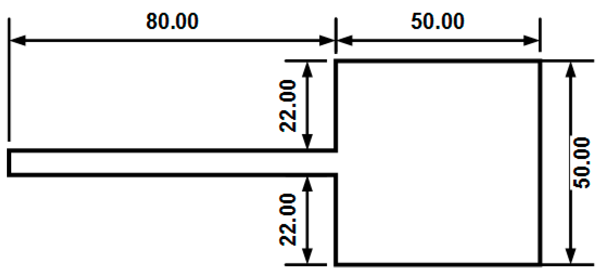
Figure 4.
Flange mounted wire-mesh probe (dimensions in mm).
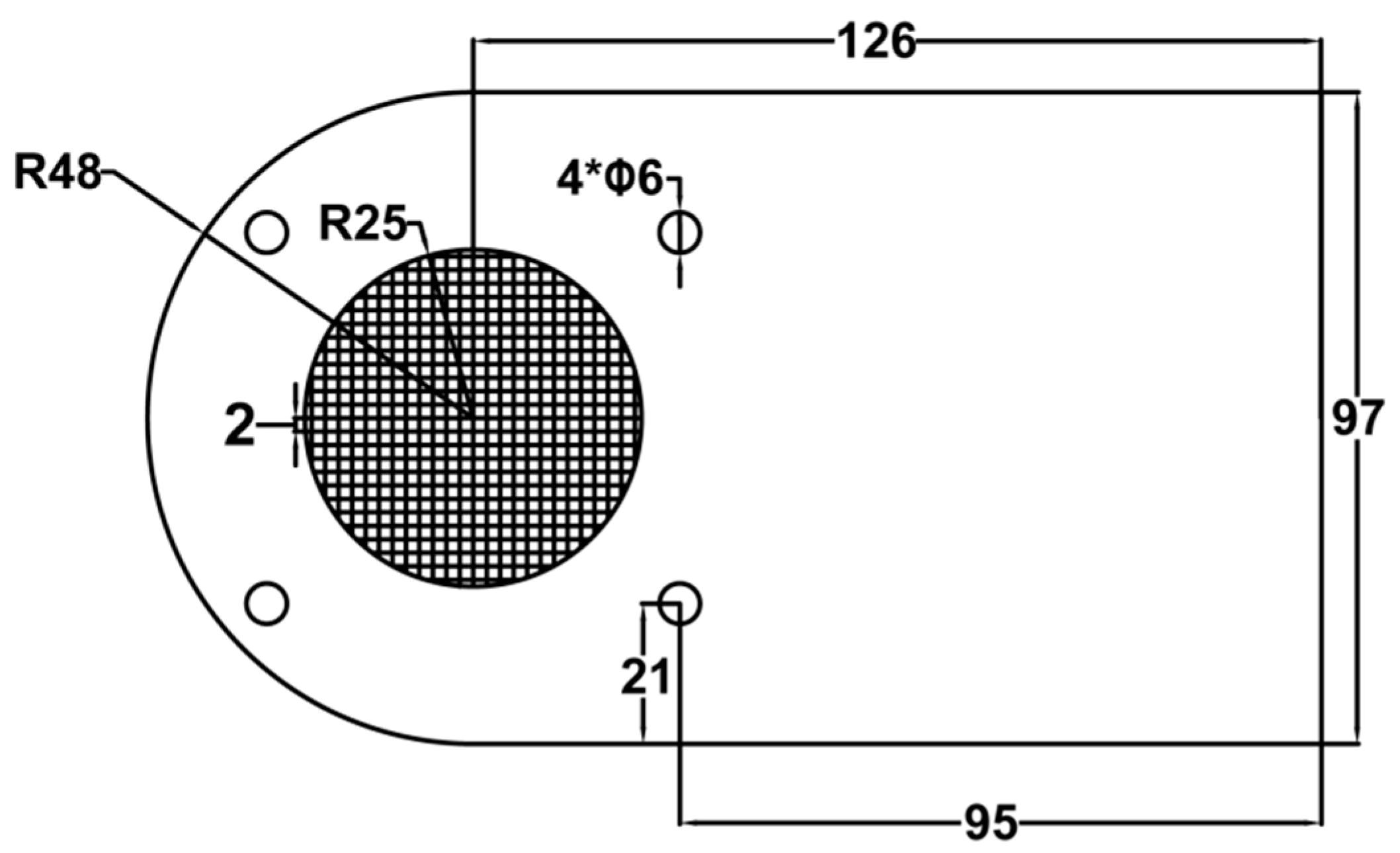
Figure 5.
Raw acoustic emission (AE) signals obtained by the T-type probe and wire-mesh probe.
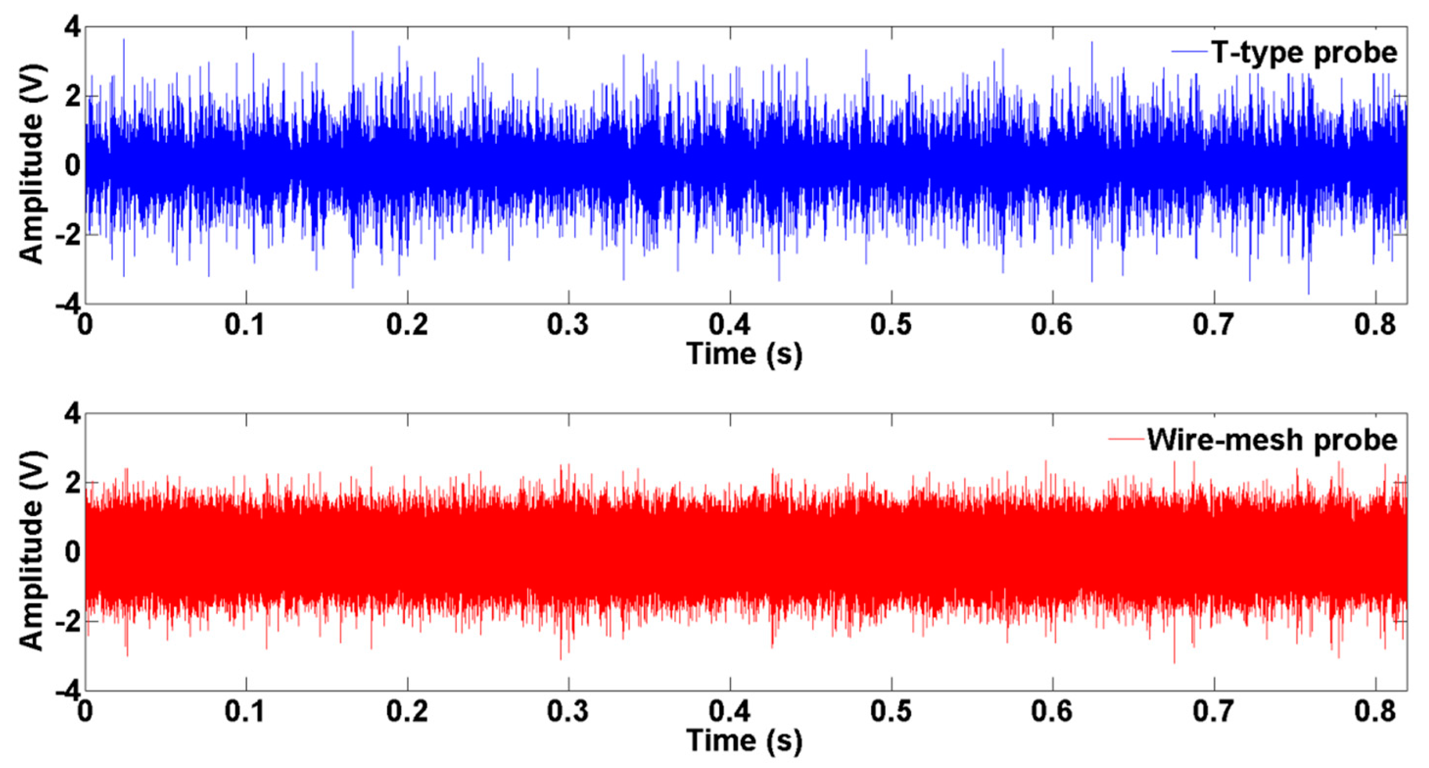
Figure 6.
Raw AE signals selected at random and divided into samples.
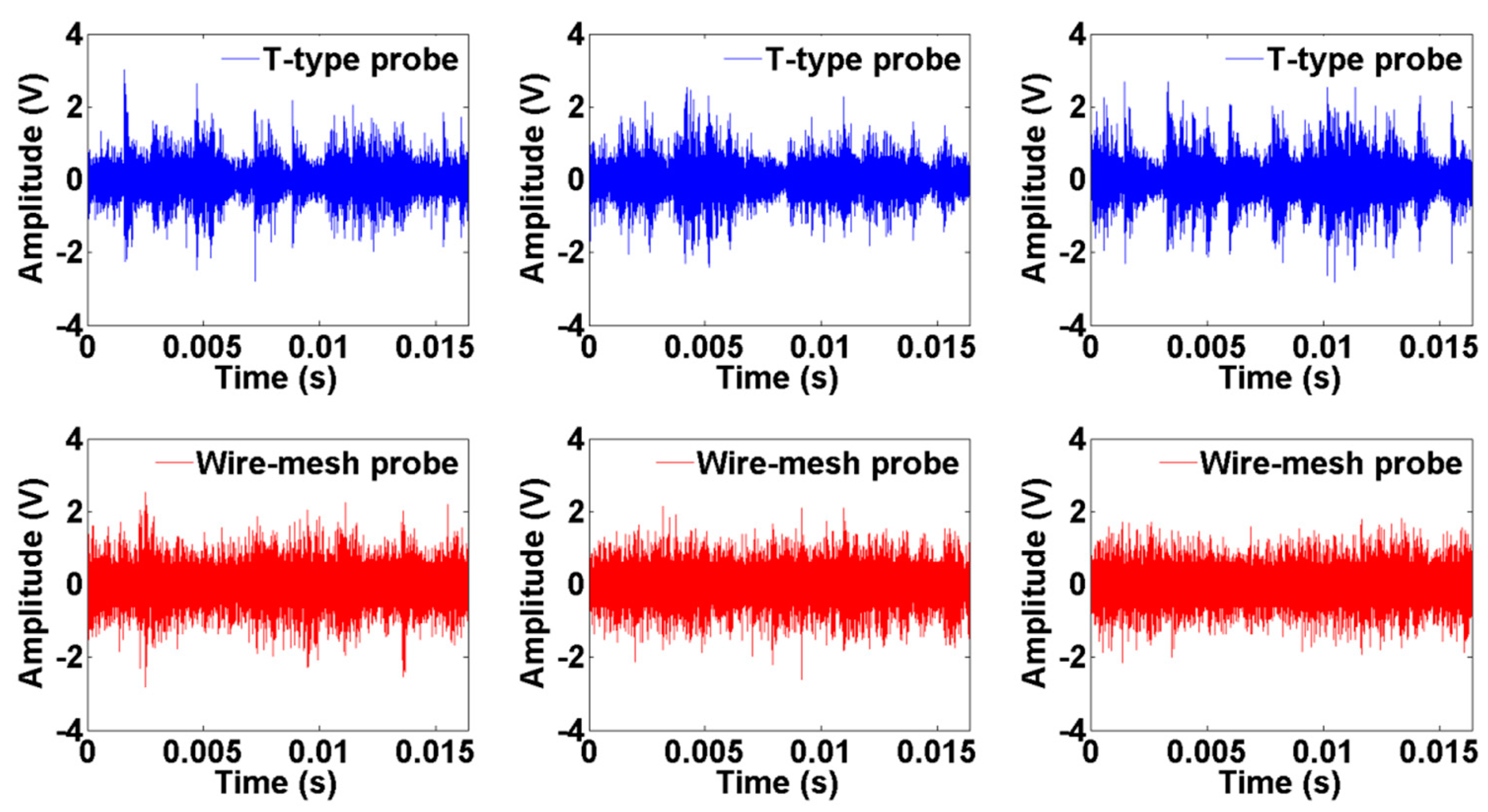
Figure 7.
(a) The root mean square (RMS) distribution and (b) the relative error for each probe type.
Figure 7.
(a) The root mean square (RMS) distribution and (b) the relative error for each probe type.
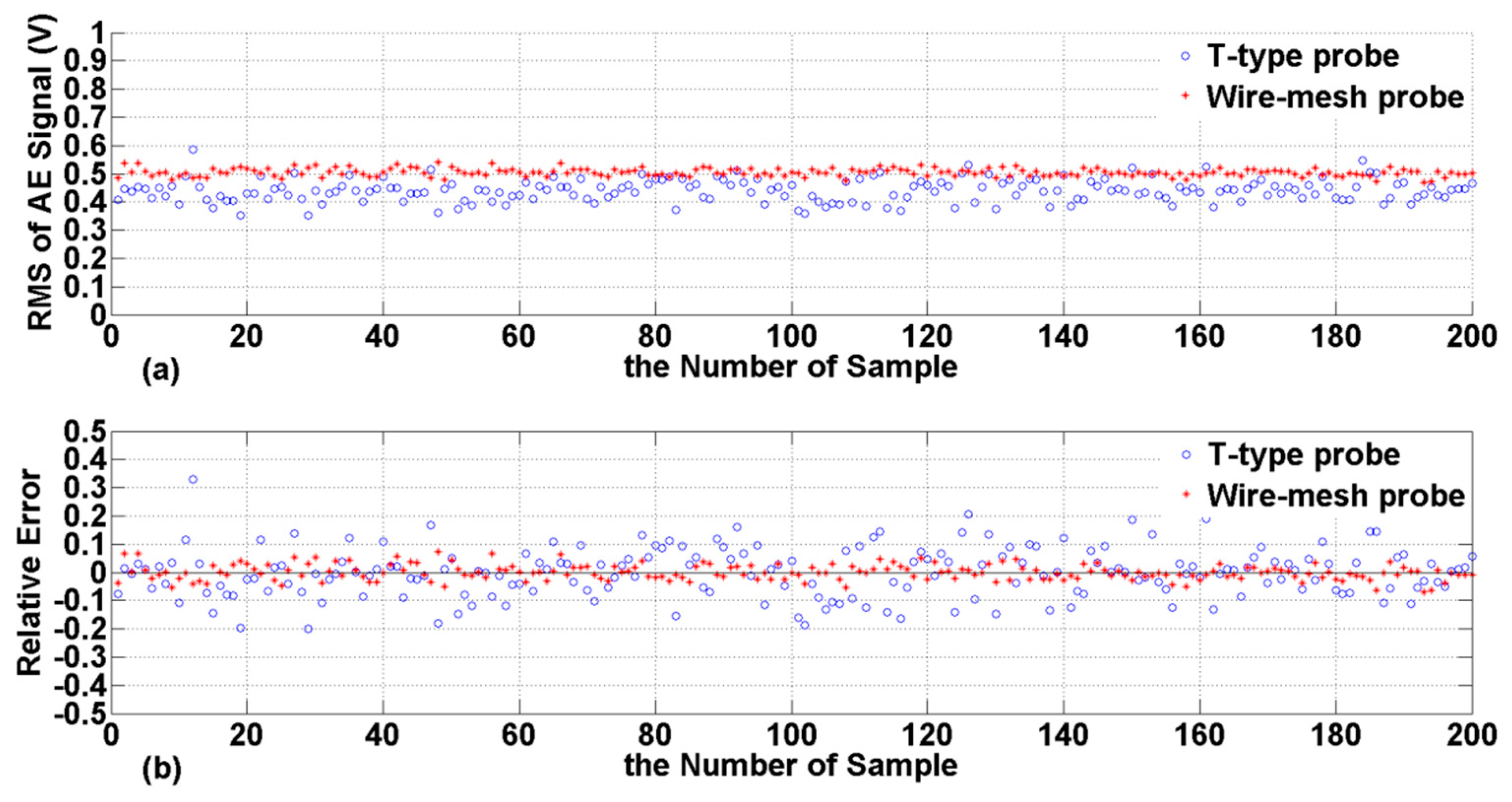
Figure 8.
The RMS average values of the AE signals with respect to particle mass flow rate at four different particle sizes.
Figure 8.
The RMS average values of the AE signals with respect to particle mass flow rate at four different particle sizes.

Figure 9.
The raw signal and the ensemble empirical mode decomposition (EEMD) signal results in time domain.
Figure 9.
The raw signal and the ensemble empirical mode decomposition (EEMD) signal results in time domain.

Figure 10.
Raw signal and a portion of the intrinsic mode functions (IMFs) in the frequency domain.
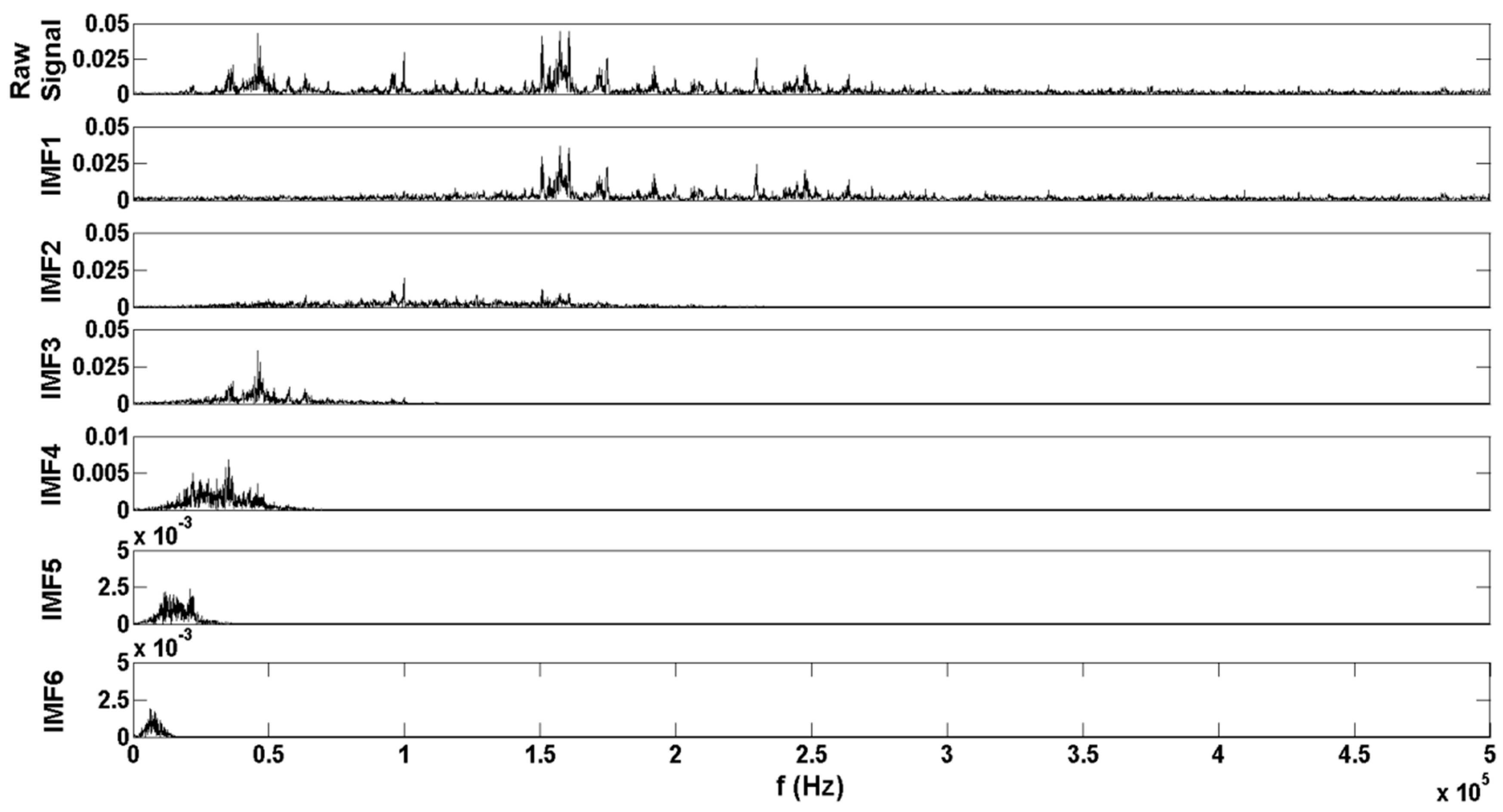
Figure 11.
Correlation coefficients between the IMF components and the raw AE signal.

Figure 12.
Relationship between IMF energy and particle mass flow rate for different particle sizes.
Figure 12.
Relationship between IMF energy and particle mass flow rate for different particle sizes.

Figure 13.
Average relative deviation from linearity for the IMF features given different particle sizes.
Figure 13.
Average relative deviation from linearity for the IMF features given different particle sizes.
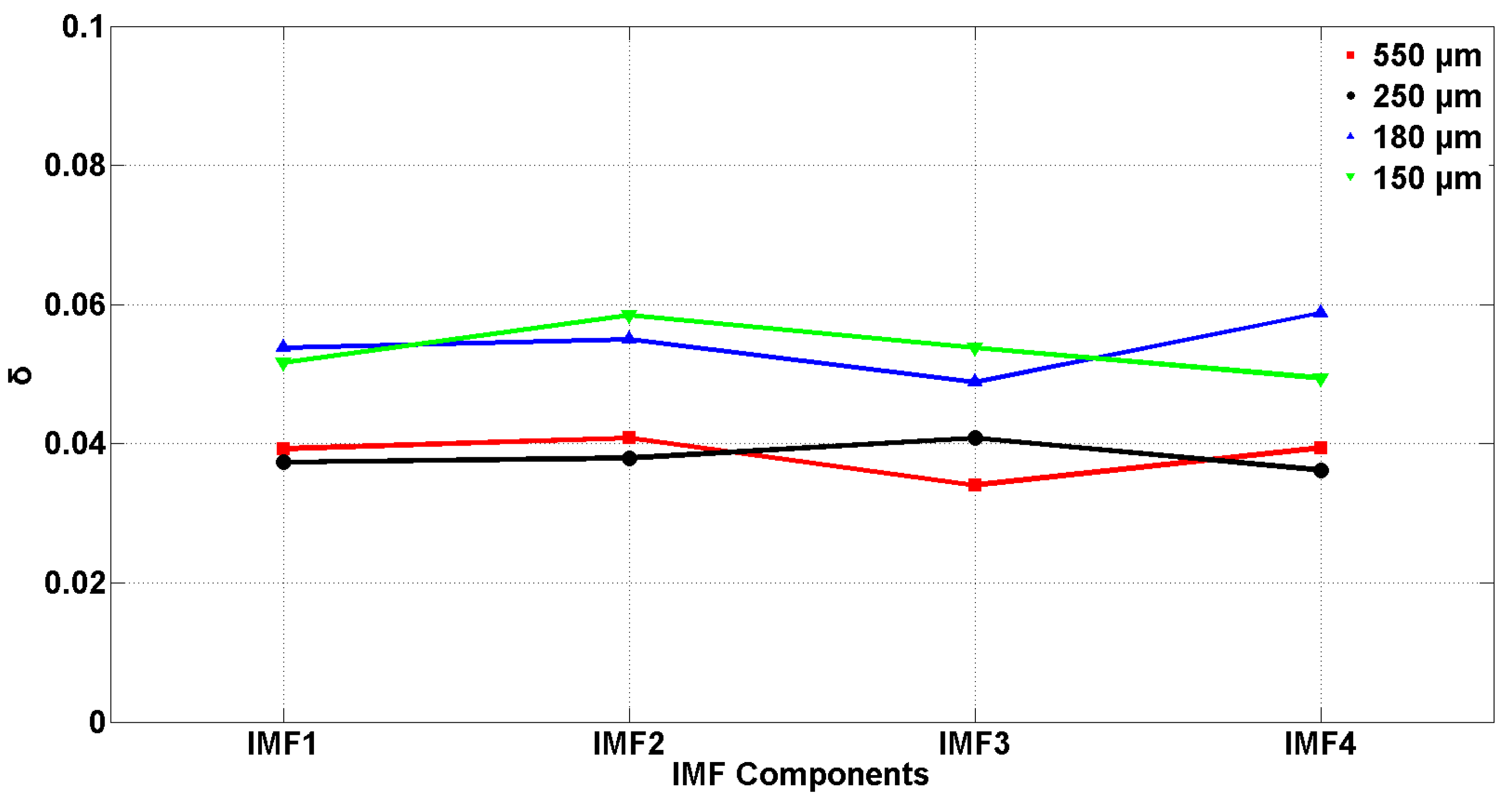
Figure 14.
Relationship between the mean-squared error contribution fraction (MSECF) for the IMFs and the particle flow rate for different particle sizes.
Figure 14.
Relationship between the mean-squared error contribution fraction (MSECF) for the IMFs and the particle flow rate for different particle sizes.

Figure 15.
Relationship between the MSECF of IMF4 and particle size with a linear fit.

Table 1.
Experimental test conditions.
| Conveying Velocity (m/s) | Particle Mass Flow Rate (g/s) | Particle Loading (%) | Particle Size (μm) |
|---|---|---|---|
| 21 | 6 to 16 with an increment of 2 | 0.006–0.016 | 550/250/180/150 |
Table 2.
Additional experiment conditions for validation.
| Conveying Velocity (m/s) | Particle Mass Flow Rate (g/s) | Particle Loading (%) | Particle Size (μm) |
|---|---|---|---|
| 21 | 18/20 | 0.018/0.02 | 550/250/180/150 |
Table 3.
Relative deviation for the validation experiments.
| Particle Mass Flow Rate (g/s) | IMF Number | 550 μm | 250 μm | 180 μm | 150 μm |
|---|---|---|---|---|---|
| 18 | IMF1 | 2.041 | 0.424 | 4.300 | 3.399 |
| IMF2 | 2.677 | 0.392 | 5.895 | 4.483 | |
| IMF3 | 2.161 | 1.726 | 4.063 | 3.176 | |
| IMF4 | 2.704 | 0.387 | 3.839 | 2.256 | |
| 20 | IMF1 | 0.580 | 5.874 | 3.784 | 4.522 |
| IMF2 | 2.474 | 6.552 | 4.852 | 4.405 | |
| IMF3 | 3.439 | 3.587 | 1.909 | 3.802 | |
| IMF4 | 1.454 | 5.532 | 4.051 | 3.620 |
Table 4.
intrinsic mode function (IMF) energy for different conditions.
| Sample Number | IMF1 | IMF2 | IMF3 | IMF4 | IMF5 | IMF6 | IMF7 | IMF8 | IMF9 |
|---|---|---|---|---|---|---|---|---|---|
| 1 | 630.921 | 98.471 | 21.726 | 5.857 | 0.725 | 0.305 | 0.186 | 0.079 | 0.050 |
| 2 | 637.792 | 97.377 | 19.765 | 5.552 | 0.775 | 0.316 | 0.163 | 0.094 | 0.053 |
© 2019 by the authors. Licensee MDPI, Basel, Switzerland. This article is an open access article distributed under the terms and conditions of the Creative Commons Attribution (CC BY) license (http://creativecommons.org/licenses/by/4.0/).
Share and Cite
MDPI and ACS Style
An, L.; Liu, W.; Ji, Y.; Shen, G.; Zhang, S. Detection of Pneumatic Conveying by Acoustic Emissions. Appl. Sci. 2019, 9, 501. https://doi.org/10.3390/app9030501
AMA Style
An L, Liu W, Ji Y, Shen G, Zhang S. Detection of Pneumatic Conveying by Acoustic Emissions. Applied Sciences. 2019; 9(3):501. https://doi.org/10.3390/app9030501
Chicago/Turabian StyleAn, Liansuo, Weilong Liu, Yongce Ji, Guoqing Shen, and Shiping Zhang. 2019. "Detection of Pneumatic Conveying by Acoustic Emissions" Applied Sciences 9, no. 3: 501. https://doi.org/10.3390/app9030501
Note that from the first issue of 2016, this journal uses article numbers instead of page numbers. See further details here.