3D U-Net for Skull Stripping in Brain MRI


1
Department of Electrical and Electronics Engineering, Hanyang University, Ansan 15588, Korea
2
Department of Mechatronics Engineering, Hanyang University, Ansan 15588, Korea
3
School of Electrical Engineering, Hanyang University, Ansan 15588, Korea
*
Author to whom correspondence should be addressed.
Appl. Sci. 2019, 9(3), 569; https://doi.org/10.3390/app9030569
Submission received: 11 December 2018
/
Revised: 1 February 2019
/
Accepted: 2 February 2019
/
Published: 8 February 2019
(This article belongs to the Special Issue Deep Learning and Big Data in Healthcare)
Abstract
:Skull stripping in brain magnetic resonance imaging (MRI) is an essential step to analyze images of the brain. Although manual segmentation has the highest accuracy, it is a time-consuming task. Therefore, various automatic segmentation algorithms of the brain in MRI have been devised and proposed previously. However, there is still no method that solves the entire brain extraction problem satisfactorily for diverse datasets in a generic and robust way. To address these shortcomings of existing methods, we propose the use of a 3D-UNet for skull stripping in brain MRI. The 3D-UNet was recently proposed and has been widely used for volumetric segmentation in medical images due to its outstanding performance. It is an extended version of the previously proposed 2D-UNet, which is based on a deep learning network, specifically, the convolutional neural network. We evaluated 3D-UNet skull-stripping using a publicly available brain MRI dataset and compared the results with three existing methods (BSE, ROBEX, and Kleesiek’s method; BSE and ROBEX are two conventional methods, and Kleesiek’s method is based on deep learning). The 3D-UNet outperforms two typical methods and shows comparable results with the specific deep learning-based algorithm, exhibiting a mean Dice coefficient of 0.9903, a sensitivity of 0.9853, and a specificity of 0.9953.

1. Introduction
Brain extraction from a volumetric dataset, T1-weighted (T1W) magnetic resonance images (MRIs) in general, is called skull stripping [1]. This is important preprocessing and is typically an initial step of most brain MRI studies e.g., cortical surface reconstruction [2], brain volumetric measurement [3], tissue identification [4], brain parts identification [5], multiple sclerosis analysis [6], assessing schizophrenia [7], Alzheimer’s disease [8]. Brain MRIs exhibit superior soft tissue contrast that is not normally found in other imaging protocols, such as computed tomography (CT) or X-rays. Automatic skull stripping is a difficult task because of the obscure brain boundaries, low contrast MRIs, and absence of intensity standardization [9]. Moreover, entire brain extraction becomes more challenging when MRI datasets with a pathological disorder are used [10].
After the pioneering results of Krizhevsky et al. [11], deep learning, particularly convolutional neural network (CNN)-based algorithms, has become a commonly used algorithmic approach to resolve medical imaging problems and challenges [12]. CNN-based algorithms are trained with known labeled data to learn the underlying mathematical description required for object or region detection, classification, and segmentation [13]. Generally, these algorithms require a vast amount of properly labeled data to train from scratch. However, biomedical image data is usually not sufficient for this challenge. Problems often worsen because labeling data requires a substantial manual effort from a brain anatomy expert in order to accomplish this tedious task [14]. Moreover, manual delineation of the brain from MRI is known to alter, even among trained individuals, and be affected by both intra- and inter-rater variabilities. For skull stripping in brain MRIs, manual segmentation of the brain is often considered to be the “ground truth” or “gold standard” and is frequently employed to validate other semi-automatic and automatic approaches. However, manual skull stripping, although doable, is an extremely time-consuming task. It also requires an urbane knowledge of brain anatomy and is laborious to perform on a large scale. Therefore, it is neither adequate nor efficient.
Many approaches considering the problem of skull-stripping in brain MRIs have been proposed over the last two decades and are continually being developed to tackle these problems and limitations. However, every technique has a constraint owing to the enormous variability of brain MRI datasets and standard. These approaches can be broadly divided into two categories: (1) Classical or conventional approaches; and (2) CNN-based or deep learning-based approaches. Classical algorithms can be further classified into the following distinct groups: Thresholding with mathematical morphology [15,16,17], deformable surface modal based [18,19,20], template or atlas-based [21,22,23], and hybrid approaches [9,24,25]. A comprehensive survey of all the existing conventional skull-stripping methods can be seen in [26].
Mathematical morphology-based algorithms exploit thresholding, edge detection, and a series of erosion and dilation operations to isolate the skull and the brain region. For instance, Brummer et al. [27] proposed a skull-stripping algorithm based on histogram-thresholding followed by morphological operations. Park and Lee [28] devised an algorithm based on a two-dimensional (2D) region growing for brain T1W MRIs. Somasundaram and Kalaiselvi [29,30] developed brain extraction algorithm (BEA) for T1W and T2-weighted (T2W) brain MRIs using morphological operations, diffusion, and connected component analysis. Shattuck et al. devised an algorithm called the Brain Surface Extractor (BSE) [31] that uses anisotropic diffusion filtering, edge detection, and a series of morphological operations to recognize the brain. BSE is extremely fast and generates highly explicit whole brain segmentation. The main drawback of this technique is that it generally requires parameter tuning to work on a particular dataset. In summary, morphological operations are highly dependent on the size and shape of the structuring element that directly influences the brain extraction results of these algorithms.
The brain extraction tool (BET) [32] is the most prevalent algorithm based on deformable surface modal-based methods. It applies locally adopted model forces to fit the surface of the brain employing a deformable model. The BET failed to segment the brain region in the inferior axial slices (slices with neck) when the center of gravity of the volume lie outside the brain. Zhuang et al. [33] proposed a model-based level set (MLS) algorithm to separate intracranial tissues and skull encircling the brain. These techniques fail to segment the brain in noisy and low-contrast MRI datasets. Generally, deformable surface modal-based methods have the potential to yield more accurate and precise skull stripping in brain MRI than approaches using mathematical morphology, edge, and thresholding.
Template or atlas-based approaches depend on a fitting template or atlas on the brain MRIs to isolate them from non-brain tissues. These methods can separate the brain from the skull when there is no well-defined relationship between the brain region and pixel intensity present in the brain MRIs. Dale et al. [21] described a brain extraction step as a preprocessing in a cortical surface reconstruction process using a tessellated ellipsoidal template. Leung et al. [23] presented a method called “Brain MAPS” that produces a brain segmentation utilizing a template library and atlas registration. Similarly, Eskildsen et al. [34] developed BEaST, a brain extraction method, based on nonlocal segmentation and a multi-resolution framework. Other recent algorithms include those mentioned in [35,36]. The accuracy of template or atlas-based approaches depends on the quality of brain mask and registration in each atlas. Furthermore, these methods are generally computationally intensive.
Hybrid approaches combine the advantages of two or more methods to increase the accuracy and precision of skull-stripping in brain MRIs. ROBEX (Robust Brain Extraction) [9] is a well-known learning-based algorithm that incorporates a discriminative (random forest) and a generative model (point distribution) with the graph cuts for skull stripping. Unfortunately, hybrid approaches often involve extensive training to learn the peculiar brain features to accurately skull strip the brain MRIs. Therefore, brain extraction remains a rate-limiting and tedious step in the brain MRIs analysis pipeline.
Recently, CNNs and deep learning-based techniques have achieved excellent performance in biomedical 2D image segmentation, with an accuracy close to human performance [37,38,39]. After successful application of CNNs on 2D biomedical images, efforts had been made on 3D biomedical volumetric data, specifically on the brain MRI [10,40]. Auto-Context CNN (Auto-Net) [41], Active Shape Model and CNN (ASM-CNN) [42], and complementary segmentation networks (CompNet) [43] are the most recently published works on brain segmentation. F. Milletari et al. [40] presented CNN with Hough voting approach that enables fully automatic localization and segmentation of a region of interest for 3D segmentation of the deep brain region. J. Kleesiek et al. [10] firstly proposed an end-to-end approach for brain extraction and skull stripping based on 3D CNN and achieved good performance. Their architecture can handle many forms including contrast-enhanced scans. Although Kleesiek’s method is the first CNN for the problem and showed state-of-the-art performance, the network is not deep. Note that the depth of network is not a problem for this specific task at hand, but it can be a problem when generalizing this network for other tasks. Generally, the shallow depth has a limited learning capability because shallow layers cannot integrate features from various levels of abstraction. Despite the immense variety of algorithms and techniques published on skull stripping, there is no consensus among the research community regarding the best method, due to obscure brain boundaries, low-contrast brain MRIs, and the absence of an intensity standardization.
In this paper, we propose the use of 3D U-Net [44], a deep network architecture designed for semantic segmentation, for skull-stripping in brain MRIs. 3D-UNet has been recently proposed and widely used for volumetric segmentation. As 2D-UNet cannot fully utilize 3D spatial information, the resulting image for the third axis is not good if the 2D-UNet is used for a 3D problem [44]. Therefore, 3D-UNet is more appropriate for skull stripping than 2D-UNet. The architecture of 3D-UNet comprises a contracting path, an expanding path, and precise localization for the good use of features in multiscale. Thus, it integrates localization and context information. 3D-UNet also uses concatenation to combine the features at high resolution with the up-sampled output to obtain local characteristics. We describe how to implement the 3D-UNet for skull-stripping in brain MRI, and how to get sufficient data for training. Then, we applied it to real publicly available brain MRI datasets and compared the brain extraction results with the three state-of-the-art widely used skull-stripping methods. Two are from classical approaches (BSE and ROBEX) and one is a CNN-based method (Kleesiek’s method) for evaluation.
2. Materials and Methods
2.1. Datasets
The performance of 3D-UNet and the other methods (BSE and ROBEX) have been evaluated on a brain MRI dataset: “Neurofeedback Skull-stripped (NFBS) repository” that is publicly available [45]. There are 125 scans of 77 females and 48 males in the 21–45 age range (average: 31 years) with a variety of clinical and subclinical psychiatric symptoms. Each subject data comprises of skull-stripped T1-weighted images along with the manually corrected gold standard. The size of the individual scan is 256 × 256 × 192 and each voxel size is 1 × 1 × 1 mm3. The first two dimensions of each scan represent the individual size of a 2D slice and the third dimension indicates the total number of slices present in the scan. Initial skull-striped brain mask from T1W MRIs have been obtained using the semi-automated skull stripping software BEaST [34]. The results were checked by visual inspection and manual correction was made to the worst results using a Free-view Visualization Tool [46]. These corrected brain masks were incorporated into the BEaST library and the process was iterated until satisfactory brain masks were available for the whole image (slices). Experts and the research community have differing opinions on the standard of what to include or exclude in the brain [9]. The brain ground truth standard used for this dataset follows from the paper of Eskildsen et al. [34]. Brain tissues consist of the cerebrum, cerebellum, brainstem, internal vessels, and arteries along with the cerebrospinal fluid (CSF) in ventricles, internal cisterns, and deep sulci. Skin, skull, eyes, dura mater, external blood vessels, and nerves are included in non-brain tissues.
2.2. Volume Sampling
Volume sampling is an essential process for training the CNN. The reason for this is that more training data in the form of subvolumes is required than the number of images available. This is a big problem in biomedical images where limited image data is available. To avoid this problem, we followed the procedure as described by [47], for subvolume choice in the training data. The size of each scan in the NFBS dataset is 256 × 256 × 192 voxels. Subvolumes of size 64 × 64 × 64 voxels have been chosen. Gaussian distribution with the mean at the center of the volume (center of the brain) and a diagonal covariance of σi = 40, i ∈ [1,2,3] was utilized. After several iterations and experiments using different numbers of subvolumes in training, it was found that 1000 subvolumes are sufficient for a precise and accurate segmentation of the brain.
2.3. Network Architecture
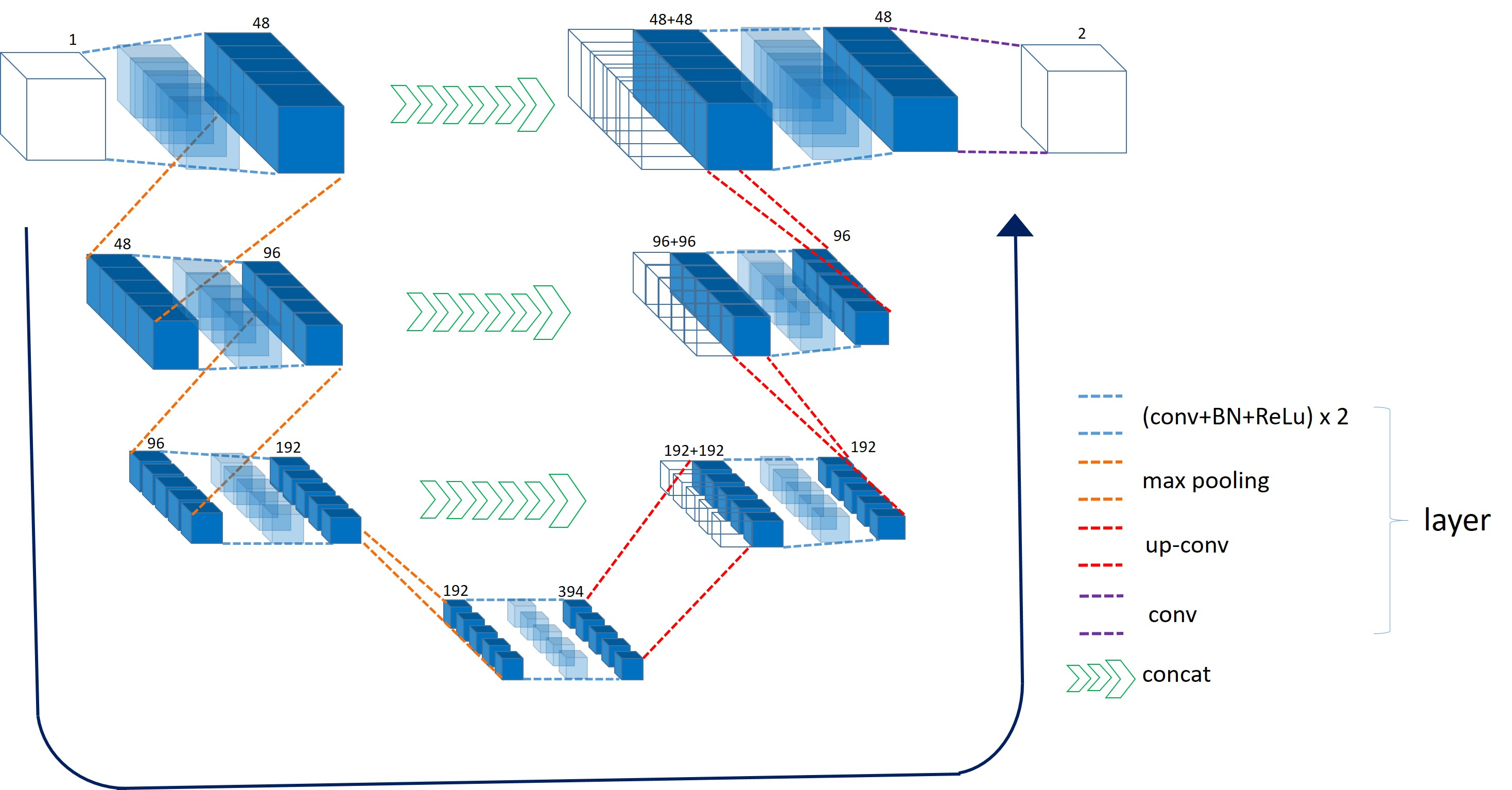
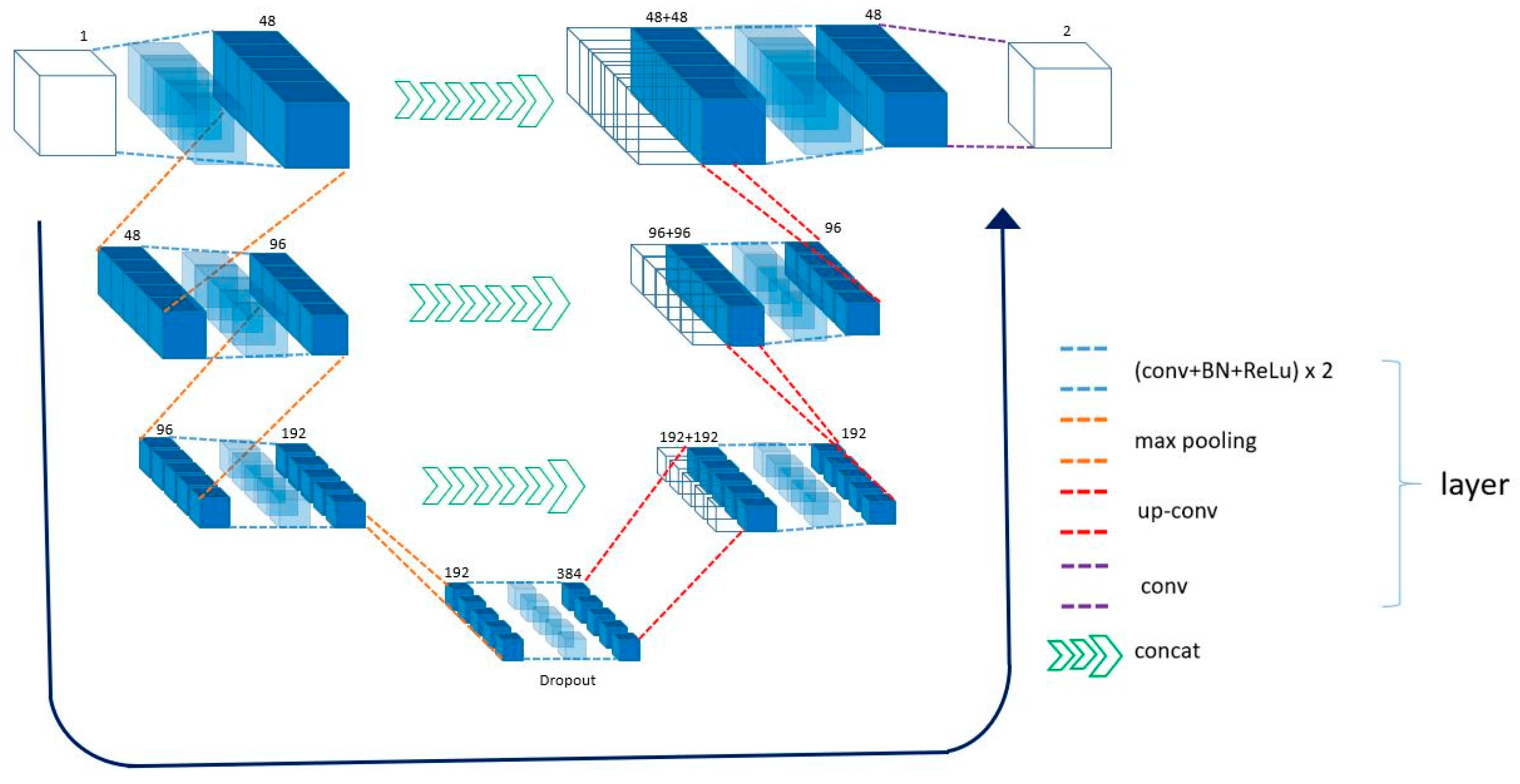
The complete network architecture is illustrated in Figure 1. There are two main parts of the network. The first part is the contracting encoder (left side in Figure 1), which extracts global features. It consists of convolution block and max pooling. A convolution block consists of convolution, batch normalization [48], and a rectified linear unit (ReLu). This was repeated two times. Batch normalization (BN) is used for faster convergence. BN is the normalization of the activation function value or the output value of the convolution. When BN is used, it is not influenced by a parameter scale during weight propagation. Thus, the learning rate that controls how much we adjust the weights can be increased, enabling rapid learning. In our training, the decay value of the BN was set to 0.9. The convolution filter size was 3 × 3 × 3 voxels. The max pooling employed for downsampling, has the size of 3 × 3 × 3 voxels with a stride of 2 in each dimension. Although max pooling has the advantage of reducing computational volume and adding robustness to noise, it has the disadvantage of losing important information. After many experiments, we found that three max pooling operations (in each dimension) are the most appropriate.
The number of feature channels is doubled after each downsampling. The dropout layer follows the fourth convolutional block. Dropout is a regularization technique to avoid overfitting [49]. Overfitting refers to the case where the model fits very well with the training dataset but does not perform well with test dataset. The reason for this is that the model is excessively optimized and fit for the training dataset. Therefore, it only works for the training dataset. The dropout technique intentionally drops out some units in the network in the training process to reduce the overfitting. Dropout improves performance by virtually creating many models and executing predictions. Learning by one model may inevitably lead to overfitting. However, if multiple models are trained and predictions with each model are made, then the risk of overfitting can be reduced. Dropout is good for training, but it generally takes more training time. Therefore, we applied dropout once at the fourth layer because the most concentrated features appear after the fourth layer.
The second part is the decoder (right in Figure 1) called expanding path in which each step consists of up convolution, concatenation with the respective cropped feature map from the encoder part, and the two convolution blocks. In CNNs, the convolution layer reduces the size of the feature map through convolution. Up convolution, however, increases the size of the feature map. It works in a way that it makes zero-padding around each pixel followed by convolution on the padded image. The final convolution filter size is 1 × 1 × 1. It is designed to get the desired class number from 64 features.
2.4. Training
Adam optimizer of the TensorFlow framework was employed for network training [50]. A variant of popular nonparametric non-uniform intensity normalization (N3) algorithm [51] was used for bias field correction. The algorithm works quite well when the brain mask is available. Therefore, we apply the method to the input sample (see Table 1 for details). The network output was generated by using the softmax and cross-entropy that are both standard in machine learning. The output of SoftMax function is compared with the ground truth labels using weighted cross-entropy loss. First, we assign k pairs of the training images (X) and labels (Y) as . Then, we flatten into a one-dimensional (1D) vector. Similarly, are also flattened into 1D vector., where i, j are the voxel and the image order, respectively. For each image, the posterior probability of voxel i with label l computed by the SoftMax classifier can be written:
where is the CNN computation function, is the patch of the voxel i and is the class number.
The output value of the SoftMax function is a real number between 0 and 1, and the sum of the all the values is 1. The weighted cross-entropy loss function is written as follows:
Since the cross-entropy between the actual distribution q and the estimated distribution p is and the actual distribution is 1 for ground truth, and 0 otherwise.
Weights are initialized using truncated normal distribution. The standard deviation of the random values was set to 0.1. Out of 125 scans, 105 scans were randomly selected for training the network and the remaining 20 scans for testing. We ran about 420,000 training iterations on two NVIDIA 1080Ti GPUs (NVIDIA Corp., Santa Clara, CA, USA, 2018), which took approximately two days.
3. Experimental Results and Discussion
The implementation of some popular and prevalent skull-stripping methods is publicly available. We considered two classical non-deep learning methods, i.e., BSE [31] and ROBEX [9], and one deep learning based method, i.e., Kleesiek’s method [10], for comparison with the presented algorithm. BSE uses anisotropic diffusion filtering, edge detection, and a series of morphological operation to recognize the brain. BSE is extremely fast and generates highly explicit whole brain segmentation. BSE in the BrainSuite16a1 [52] package have been chosen with the default parameters (diffusion iteration = 3, diffusion constant = 25, edge constant = 0.64, erosion Size 1) for skull stripping. ROBEX is a learning-based brain extraction system in which a discriminative (random forest) and a generative model (point distribution) are combined to achieve skull stripping. The contour of the brain is further refined by graph cuts. It shows improved performance without any parameter tuning. ROBEX1.2 package available at [53] was used for this comparison. The Kleesiek’s method is to use a specifically designed deep learning network for skull stripping [10]. Note that we also considered BET [32] for comparison but the results were worst on this dataset. Thus, we have not included it in this comparison.
3.1. Evaluation Metrics
For quantitative evaluation of automatically extracted brain with the ground truth, three overlap metrics were computed, i.e., Dice coefficient, sensitivity, and specificity. The adopted metrics evaluate various performance characteristics between the extracted brain by the algorithms and the manual annotation (ground truth) brain segmentation. Sensitivity and specificity were used to measure the rate of classification (or misclassification) of the brain. The compromise between specificity and sensitivity metrics is a Dice coefficient; it assesses the tradeoff between the incorrect and the correct voxel segmentations.Dice coefficient measures the overlap between the ground truth and segmentation results obtained from the algorithm. It can be defined by using the notion of true positive (TP), false positive (FP), and false negative (FN) as:
where TP = Pixels correctly classified as a brain in ground truth and by algorithm; FP = Pixels not classified as a brain in ground truth but classified as brain by the algorithm; TN = Pixels not classified as a brain in ground truth and by algorithm; FN = Pixels classified as a brain in ground truth, but not classified as brain by the algorithm.
Table 2 and Table 3 show Dice score for all the 20 test scans for proposed (3D-UNet), BSE, ROBEX and Kleesiek’s method, respectively. The value of Dice coefficient varies from 0 (disjoint or complete disagree) to 1(for complete overlap or agreement).
Sensitivity is also known as TP rate. It measures the proportion or percentage of the TPs that are correctly classified as the brain. Mathematically, it can be written as:
Specificity is also known as TN rate. It measures the proportion or percentage of the TNs that are correctly classified as non-brain. Mathematically, it can be written as:
3.2. Quantitative Results
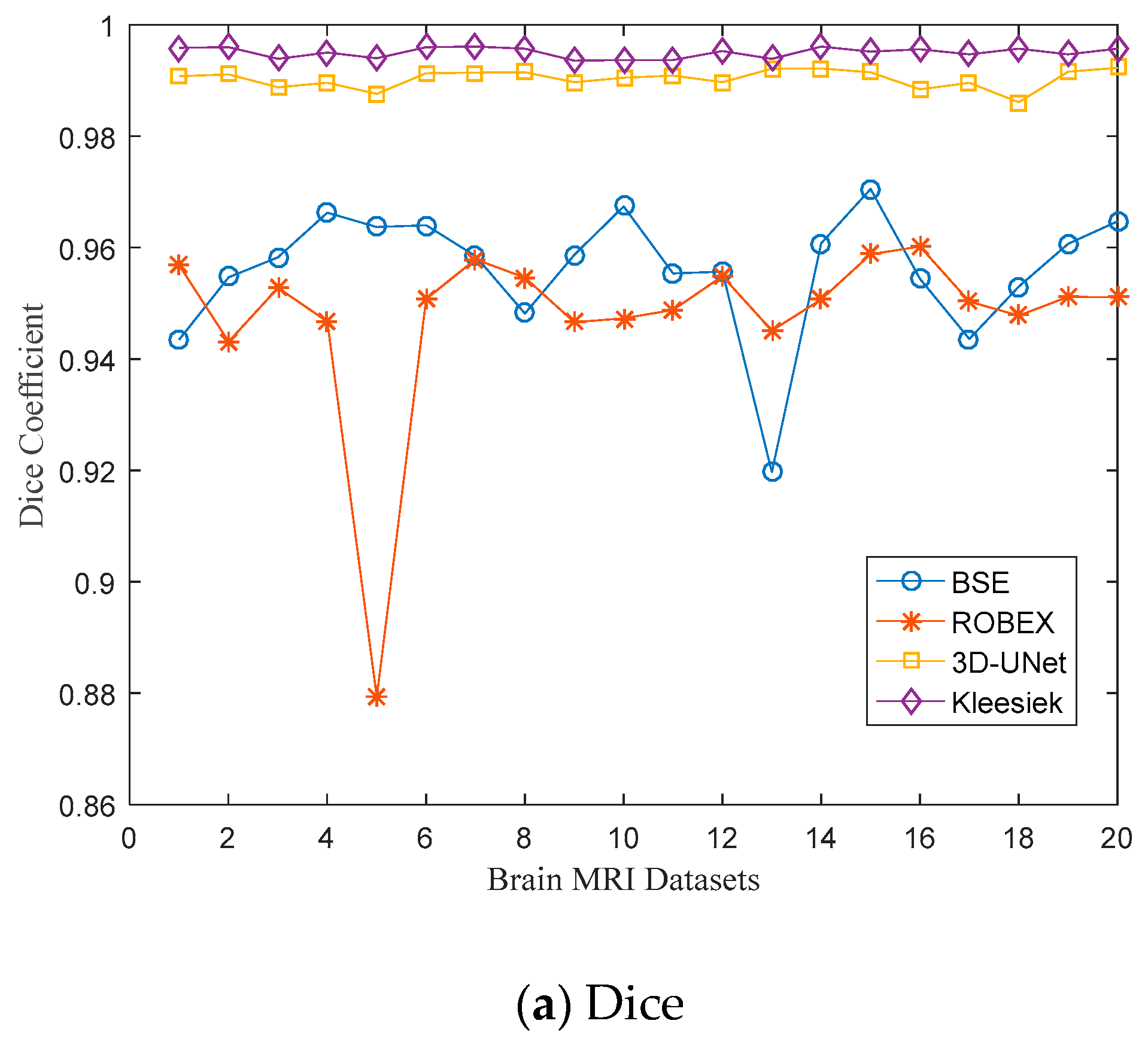
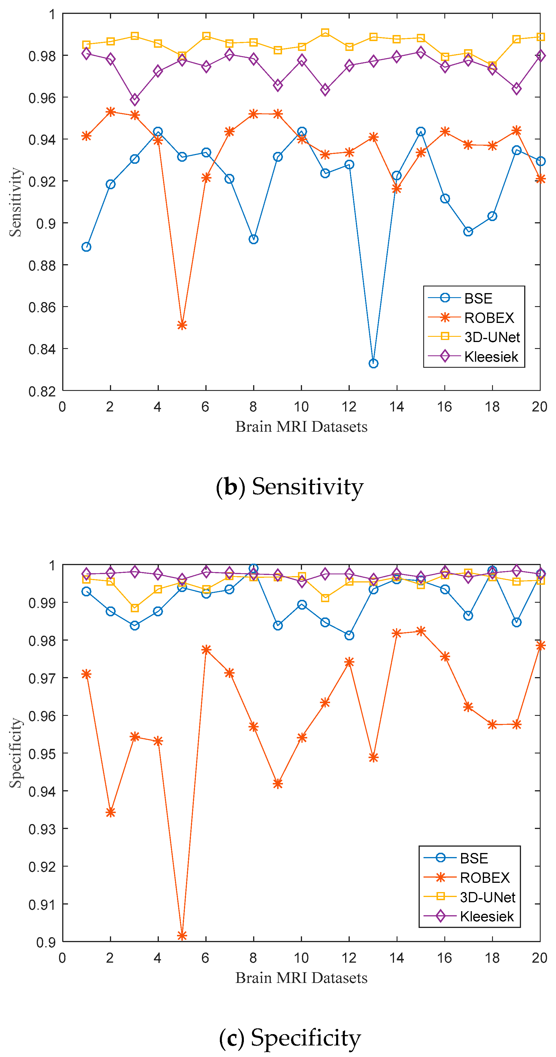
Table 2 summarizes the overall analysis for each evaluated metric i.e., Dice, sensitivity, and specificity, respectively. The plot of these measurements for the individual test scan is illustrated in Figure 2. Performance of the 3D-UNet method was excellent with respect to Dice, sensitivity, and specificity, across all the test datasets; the conventional methods (BSE and ROBEX) generally performed well (i.e., > 0.9 on Dice coefficient, sensitivity, and specificity). BSE shows a better Dice score as compared to ROBEX, particularly, the Dice score for scan 5 is substantially different (0.8793) as depicted in Figure 2a. The overall sensitivity values of ROBEX for test scans is relatively greater than BSE. This indicates that ROBEX classified the brain tissues more accurately and segmented most of the brain because the sensitivity assesses how much brain tissue is included in the brain segmentation.
On the other hand, the specificity scores of BSE is much better than the ROBEX. This represents that BSE segmented the non-brain tissues more correctly and excluded most of the non-brain region compared to ROBEX. Moreover, BSE and ROBEX failed to correctly segment the brain in the initial slices of the brain MRI volume. The Dice score in the slices (40–45% of the total slices contains brain tissues) for both the competitor algorithms is less than 0.90 (on average) as displayed in Figure 3. In contrary, the 3D-UNet shows a consistent performance in all the slices either from the start or at the end of the brain MRI volume. Figure 3 portrayed the slice-by-slice Dice score comparison of the individual algorithm with 3D-UNet.
The overall quantitative performance of the 3D-UNet with ROBEX and BSE is shown in Table 2. Best values (results) in the respective category are emboldened. Figure 2 demonstrates corresponding plots for each algorithm, including all the test brain MRI scans. The proposed algorithm achieved the highest average Dice, sensitivity, and specificity score with a significant difference when compared with BSE and ROBEX. Sensitivity value for BSE is smaller than the other methods and indicates that it has excluded several brain tissues than the other methods. Specificity value for ROBEX is substantially small for test dataset (scan 5) and implies that it has included more non-brain tissues than the other methods. Table 3 shows the comparison results of Kleesiek’s method and 3D-UNet. Both deep learning-based methods show excellent performance compared to classical methods. Kleesiek’s method seems to be a little superior in terms of dice coefficient and specificity. The sensitivity value of 3D-UNet was a little better as compared to Kleesiek’s algorithm. In conclusion, the results of both the CNNs-based methods are comparable and outperformed the classical best skull stripping algorithms.
3.3. Qualitative Results.
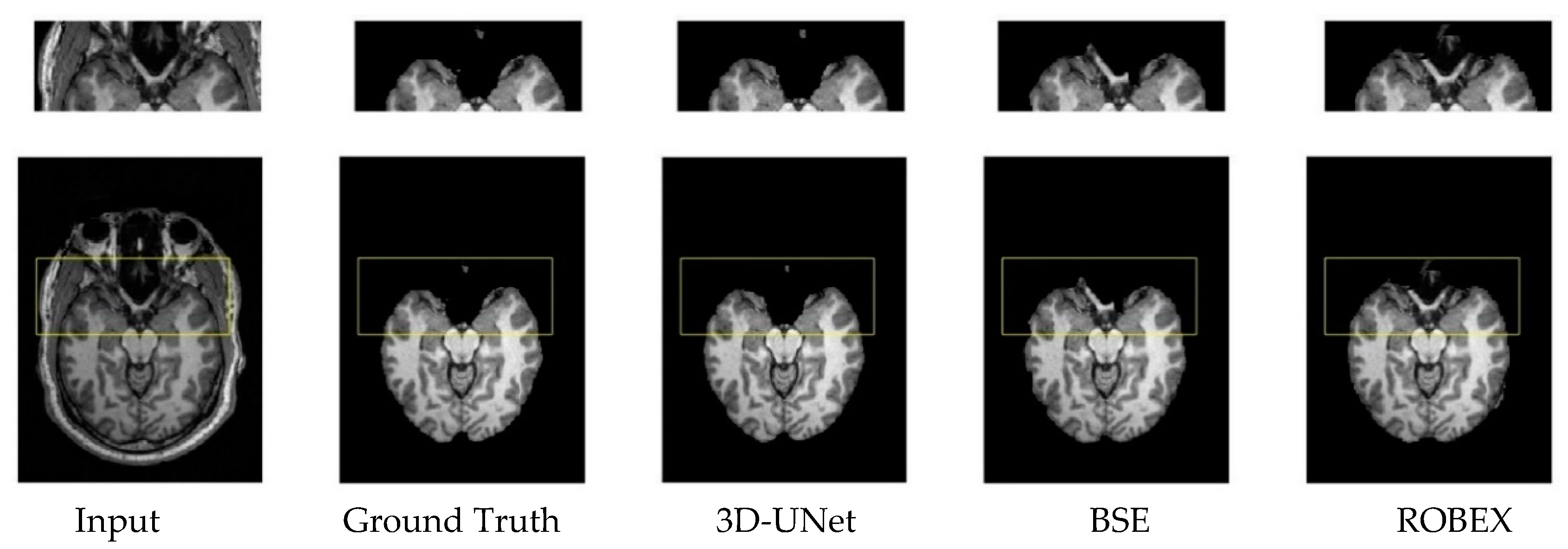
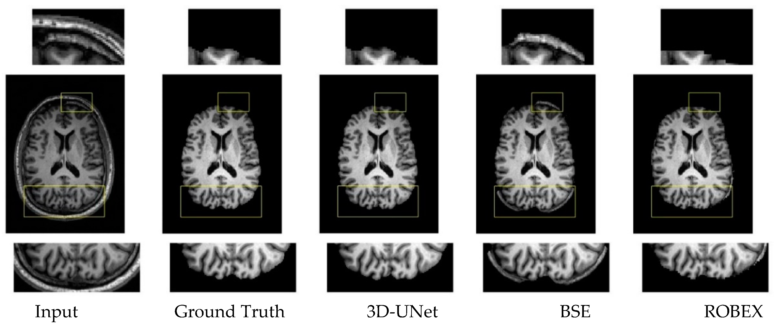
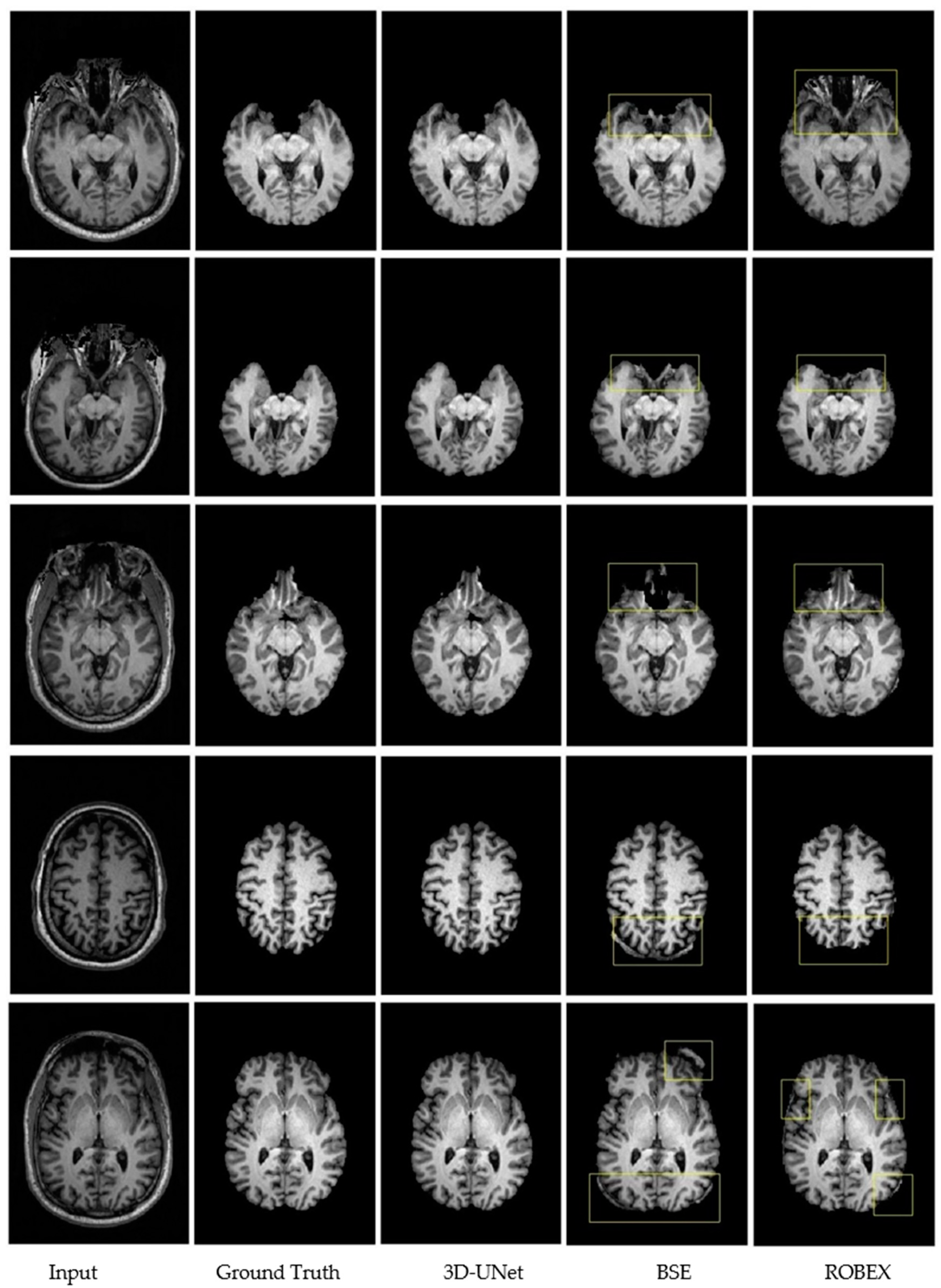
For the qualitative performance of the proposed method and comparison with other algorithms, some orthogonal slices from the test data are depicted in Figure 4–7. The first and second column of the figure displays input and ground truth orthogonal slices, from different scans, respectively. Last three columns show brain extraction results from the 3D-UNet, BSE, and ROBEX, respectively. One important aspect of both the algorithms (ROBEX and BSE) is that their segmentation in the inferior (eyes images) and superior slices are not good, and show mediocre performance as shown in Figure 4 and Figure 5. The failure region (under or over-segmentation of the brain) have been indicated with a rectangle and displayed in a zoom view. The 3D-UNet produces more accurate and smooth generation of brain compared to BSE and ROBEX.
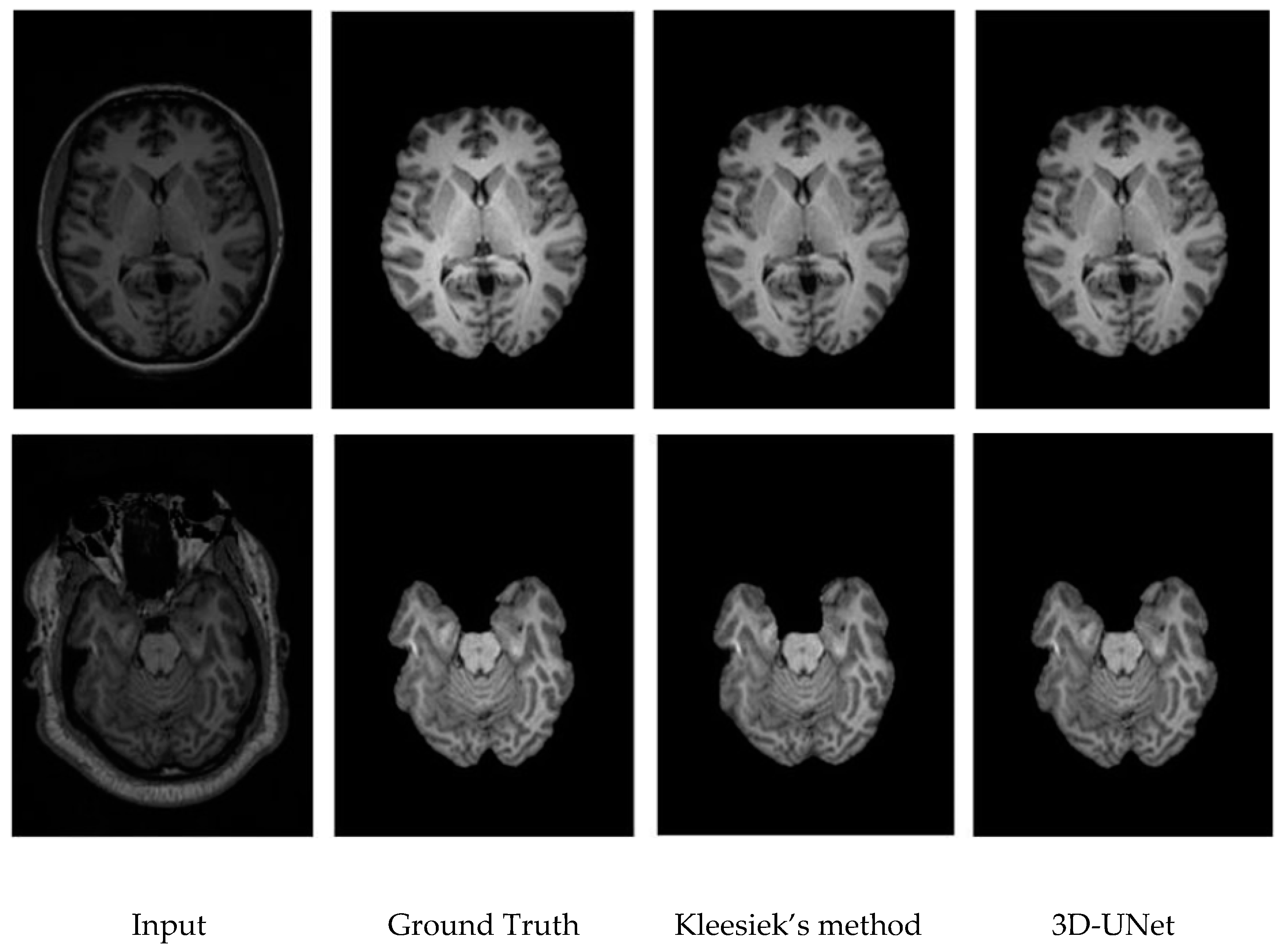
ROBEX shows improved performance without any parameter tuning. One disadvantage of the ROBEX is that it smooths gyri and sulci (contour of the brain) excessively that lead to the inclusion of non-brain tissue dura and/or gray matter loss, as represented in Figure 4. BSE also failed when no significant difference was present between the intensities of the brain and non-brain edges. Furthermore, the skull-stripping results of both the algorithms are not consistent. ROBEX had a high sensitivity but poor Dice coefficient (overlap) and specificity. Similarly, BSE had greater score of specificity but low sensitivity and Dice coefficient values. On the other hand, the brain extraction results of both CNN-based algorithms are excellent and consistent in either case, i.e., the brain slices with eyes or without eyes, as shown in Figure 6. BSE is the fastest among the compared algorithms. It took only a 3.5(±0.4) s for the whole brain extraction. 3D-UNet and ROBEX spent 228(±0.5) s and 73.8(±1.6) s, respectively. 3D-UNet takes more time in skull-stripping due to deep CNNs structure, but its good performance and results are worth considering, and using it for skull-stripping. Figure 7 shows one result example of qualitative comparison of 3D U-Net and Kleesiek’s methods. Both deep learning-based methods perform outstandingly well, showing little difference with ground truth.
4. Conclusions
We proposed the use of 3D-UNet, an end-to-end deep learning-based segmentation algorithm for skull stripping. The method is fully automatic and has shown successful skull-stripping in real MRI datasets of the brain. The presented method has been compared with the two most popular conventional and one deep learning based methods. 3D-UNet outperformed the classical methods in terms of its Dice coefficient, sensitivity and specificity. It also shows comparable results with a specifically designed deep network for the problem. In future, we will deal with brain MRIs for pathological disorders. Although the presented deep learning-based technique is a little slow compared to existing non-deep learning algorithms, its excellent performance is worth considering and using for skull stripping. Optimization of the network to make it faster also remains a future work.
Author Contributions
H.H. proposed the idea, and implemented it. H.Z.U.R. contributed to the comparative analysis and wrote the manuscript. S.L. supervised the study and the manuscript-writing process, and made suggestions in manuscript correction and improvements.
Funding
This work was funded by the Korean Government under Grant No. 2015R1C1A1A01056013 (MSIT), Grant No. 2012M3A6A3055694 (MSIT), and 20001856 (MOTIE).
Acknowledgments
We thank the Ministry of Science and ICT (MSIT) and the Ministry of Trade, Industry and Energy (MOTIE) of the Korean Government for the financial support. We also thank the Higher Education Commission (HEC) of Pakistan for HRDI-UESTPs.
Conflicts of Interest
The authors declare no conflict of interest.
References
- Uhlich, M.; Greiner, R.; Hoehn, B.; Woghiren, M.; Diaz, I.; Ivanova, T.; Murtha, A. Improved Brain Tumor Segmentation via Registration-Based Brain Extraction. Forecasting 2018, 1, 59–69. [Google Scholar] [CrossRef]
- Tosun, D.; Rettmann, M.E.; Naiman, D.Q.; Resnick, S.M.; Kraut, M.A.; Prince, J.L. Cortical reconstruction using implicit surface evolution: Accuracy and precision analysis. Neuroimage 2006, 29, 838–852. [Google Scholar] [CrossRef] [PubMed]
- Kalkers, N.F.; Ameziane, N.; Bot, J.C.J.; Minneboo, A.; Polman, C.H.; Barkhof, F. Longitudinal brain volume measurement in multiple sclerosis—Rate of brain atrophy is independent of the disease subtype. Arch. Neurol. 2002, 59, 1572–1576. [Google Scholar] [CrossRef] [PubMed]
- Wang, L.; Chen, Y.; Pan, X.; Hong, X.; Xia, D. Level set segmentation of brain magnetic resonance images based on local Gaussian distribution fitting energy. J. Neurosci. Methods 2010, 188, 316–325. [Google Scholar] [CrossRef] [PubMed]
- Zhao, L.; Ruotsalainen, U.; Hirvonen, J.; Hietala, J.; Tohka, J. Automatic cerebral and cerebellar hemisphere segmentation in 3D MRI: Adaptive disconnection algorithm. Med. Image Anal. 2010, 14, 360–372. [Google Scholar] [CrossRef] [PubMed]
- Zhou, F.; Zhuang, Y.; Gong, H.; Zhan, J.; Grossman, M.; Wang, Z. Resting State Brain Entropy Alterations in Relapsing Remitting Multiple Sclerosis. PLoS ONE 2016, 11, e0146080. [Google Scholar] [CrossRef] [PubMed]
- Tanskanen, P.; Veijola, J.M.; Piippo, U.K.; Haapea, M.; Miettunen, J.A.; Pyhtinen, J.; Bullmore, E.T.; Jones, P.B.; Isohanni, M.K. Hippocampus and amygdala volumes in schizophrenia and other psychoses in the Northern Finland 1966 birth cohort. Schizophr. Res. 2005, 75, 283–294. [Google Scholar] [CrossRef]
- Rusinek, H.; de Leon, M.J.; George, A.E.; Stylopoulos, L.A.; Chandra, R.; Smith, G.; Rand, T.; Mourino, M.; Kowalski, H. Alzheimer disease: Measuring loss of cerebral gray matter with MR imaging. Radiology 1991, 178, 109–114. [Google Scholar] [CrossRef]
- Iglesias, J.E.; Liu, C.Y.; Thompson, P.M.; Tu, Z. Robust brain extraction across datasets and comparison with publicly available methods. IEEE Trans. Med. Imaging 2011, 30, 1617–1634. [Google Scholar] [CrossRef]
- Kleesiek, J.; Urban, G.; Hubert, A.; Schwarz, D.; Maier-Hein, K.; Bendszus, M.; Biller, A. Deep MRI brain extraction: A 3D convolutional neural network for skull stripping. Neuroimage 2016, 129, 460–469. [Google Scholar] [CrossRef]
- Krizhevsky, A.; Sutskever, I.; Hinton, G.E. ImageNet classification with deep convolutional neural networks. In Proceedings of the 25th International Conference on Neural Information Processing Systems, Lake Tahoe, NV, USA, 3–6 December 2012; Volume 1, pp. 1097–1105. [Google Scholar]
- Litjens, G.; Kooi, T.; Bejnordi, B.E.; Setio, A.A.A.; Ciompi, F.; Ghafoorian, M.; van der Laak, J.; van Ginneken, B.; Sanchez, C.I. A survey on deep learning in medical image analysis. Med. Image Anal. 2017, 42, 60–88. [Google Scholar] [CrossRef] [PubMed]
- LeCun, Y.; Bengio, Y.; Hinton, G. Deep learning. Nature 2015, 521, 436–444. [Google Scholar] [CrossRef] [PubMed]
- Greenspan, H.; van Ginneken, B.; Summers, R.M. Guest Editorial Deep Learning in Medical Imaging: Overview and Future Promise of an Exciting New Technique. IEEE Trans. Med. Imag. 2016, 35, 1153–1159. [Google Scholar] [CrossRef]
- Dawant, B.M.; Hartmann, S.L.; Thirion, J.P.; Maes, F.; Vandermeulen, D.; Demaerel, P. Automatic 3-D segmentation of internal structures of the head in MR images using a combination of similarity and free-form transformations: Part I, methodology and validation on normal subjects. IEEE Trans. Med. Imag. 1999, 18, 909–916. [Google Scholar] [CrossRef]
- Grau, V.; Mewes, A.U.J.; Alcaniz, M.; Kikinis, R.; Warfield, S.K. Improved watershed transform for medical image segmentation using prior information. IEEE Trans. Med. Imag. 2004, 23, 447–458. [Google Scholar] [CrossRef] [PubMed]
- Shan, Z.Y.; Yue, G.H.; Liu, J.Z. Automated histogram-based brain segmentation in T1-weighted three-dimensional magnetic resonance head images. Neuroimage 2002, 17, 1587–1598. [Google Scholar] [CrossRef] [PubMed]
- Aboutanos, G.B.; Nikanne, J.; Watkins, N.; Dawant, B.M. Model creation and deformation for the automatic segmentation of the brain in MR images. IEEE Trans. Biomed. Eng. 1999, 46, 1346–1356. [Google Scholar] [CrossRef] [PubMed]
- Suri, J.S. Two-dimensional fast magnetic resonance brain segmentation. IEEE. Eng. Med. Biol. Mag. 2001, 20, 84–95. [Google Scholar] [CrossRef] [PubMed]
- Merisaari, H.; Parkkola, R.; Alhoniemi, E.; Teras, M.; Lehtonen, L.; Haataja, L.; Lapinleimu, H.; Nevalainen, O.S. Gaussian mixture model-based segmentation of MR images taken from premature infant brains. J. Neurosci. Methods 2009, 182, 110–122. [Google Scholar] [CrossRef] [PubMed]
- Dale, A.M.; Fischl, B.; Sereno, M.I. Cortical surface-based analysis. I. Segmentation and surface reconstruction. Neuroimage 1999, 9, 179–194. [Google Scholar] [CrossRef] [PubMed]
- Kobashi, S.; Fujimoto, Y.; Ogawa, M.; Ando, K.; Ishikura, R.; Kondo, K.; Hirota, S.; Hata, Y. Fuzzy-ASM Based Automated Skull Stripping Method from Infantile Brain MR Images. In Proceedings of the 2007 IEEE International Conference on Granular Computing (GRC 2007), San Jose, CA, USA, 2–4 November 2007; p. 632. [Google Scholar]
- Leung, K.K.; Barnes, J.; Modat, M.; Ridgway, G.R.; Bartlett, J.W.; Fox, N.C.; Ourselin, S.; Initia, A.D.N. Brain MAPS: An automated, accurate and robust brain extraction technique using a template library. Neuroimage 2011, 55, 1091–1108. [Google Scholar] [CrossRef] [PubMed]
- Atkins, M.S.; Mackiewich, B.T. Fully automatic segmentation of the brain in MRI. IEEE Trans. Med. Imag. 1998, 17, 98–107. [Google Scholar] [CrossRef] [PubMed]
- Rehm, K.; Schaper, K.; Anderson, J.; Woods, R.; Stoltzner, S.; Rottenberg, D. Putting our heads together: A consensus approach to brain/non-brain segmentation in T1-weighted MR volumes. Neuroimage 2004, 22, 1262–1270. [Google Scholar] [CrossRef]
- Kalavathi, P.; Prasath, V.S. Methods on skull stripping of MRI head scan images—A review. J. Digit. Imag. 2016, 29, 365–379. [Google Scholar] [CrossRef] [PubMed]
- Brummer, M.E.; Mersereau, R.M.; Eisner, R.L.; Lewine, R.J. Automatic detection of brain contours in MRI data sets. IEEE Trans. Med. Imaging 1993, 12, 153–166. [Google Scholar] [CrossRef] [PubMed]
- Park, J.G.; Lee, C. Skull stripping based on region growing for magnetic resonance brain images. Neuroimage 2009, 47, 1394–1407. [Google Scholar] [CrossRef]
- Somasundaram, K.; Kalaiselvi, T. Fully automatic brain extraction algorithm for axial T2-weighted magnetic resonance images. Comput. Biol. Med. 2010, 40, 811–822. [Google Scholar] [CrossRef]
- Somasundaram, K.; Kalaiselvi, T. Automatic brain extraction methods for T1 magnetic resonance images using region labeling and morphological operations. Comput. Biol. Med. 2011, 41, 716–725. [Google Scholar] [CrossRef]
- Shattuck, D.W.; Sandor-Leahy, S.R.; Schaper, K.A.; Rottenberg, D.A.; Leahy, R.M. Magnetic resonance image tissue classification using a partial volume model. Neuroimage 2001, 13, 856–876. [Google Scholar] [CrossRef]
- Smith, S.M. Fast robust automated brain extraction. Hum. Brain Mapp. 2002, 17, 143–155. [Google Scholar] [CrossRef]
- Zhuang, A.H.; Valentino, D.J.; Toga, A.W. Skull-stripping magnetic resonance brain images using a model-based level set. Neuroimage 2006, 32, 79–92. [Google Scholar] [CrossRef] [PubMed]
- Eskildsen, S.F.; Coupe, P.; Fonov, V.; Manjon, J.V.; Leung, K.K.; Guizard, N.; Wassef, S.N.; Ostergaard, L.R.; Collins, D.L.; Alzheimer’s Disease Neuroimaging, I. BEaST: Brain extraction based on nonlocal segmentation technique. Neuroimage 2012, 59, 2362–2373. [Google Scholar] [CrossRef] [PubMed]
- Heckemann, R.A.; Ledig, C.; Gray, K.R.; Aljabar, P.; Rueckert, D.; Hajnal, J.V.; Hammers, A. Brain Extraction Using Label Propagation and Group Agreement: Pincram. PLoS ONE 2015, 10, e0129211. [Google Scholar] [CrossRef]
- Wang, Y.; Nie, J.; Yap, P.T.; Shi, F.; Guo, L.; Shen, D. Robust deformable-surface-based skull-stripping for large-scale studies. In Proceedings of the International Conference on Medical Image Computing and Computer-Assisted Intervention, Toronto, ON, Canada, 18–22 September 2011; Volume 14, pp. 635–642. [Google Scholar]
- Hariharan, B.; Arbeláez, P.; Girshick, R.; Malik, J. Hypercolumns for object segmentation and fine-grained localization. In Proceedings of the 2015 IEEE Conference on Computer Vision and Pattern Recognition (CVPR), Boston, MA, USA, 7–12 June 2015; pp. 447–456. [Google Scholar]
- Ronneberger, O.; Fischer, P.; Brox, T. U-Net: Convolutional Networks for Biomedical Image Segmentation. In Proceedings of the International Conference on Medical image computing and computer-assisted intervention, Munich, Germany, 5–9 October 2015; pp. 234–241. [Google Scholar]
- Seyedhosseini, M.; Sajjadi, M.; Tasdizen, T. Image Segmentation with Cascaded Hierarchical Models and Logistic Disjunctive Normal Networks. In Proceedings of the 2013 IEEE International Conference on Computer Vision, Sydney, NSW, Australia, 1–8 December 2013; pp. 2168–2175. [Google Scholar]
- Milletari, F.; Ahmadi, S.A.; Kroll, C.; Plate, A.; Rozanski, V.; Maiostre, J.; Levin, J.; Dietrich, O.; Ertl-Wagner, B.; Botzel, K.; et al. Hough-CNN: Deep learning for segmentation of deep brain regions in MRI and ultrasound. Comput. Vis. Image Underst. 2017, 164, 92–102. [Google Scholar] [CrossRef]
- Salehi, S.S.M.; Erdogmus, D.; Gholipour, A. Auto-Context Convolutional Neural Network (Auto-Net) for Brain Extraction in Magnetic Resonance Imaging. IEEE Trans. Med. Imag. 2017, 36, 2319–2330. [Google Scholar] [CrossRef] [PubMed]
- Duy, N.H.M.; Duy, N.M.; Truong, M.T.N.; Bao, P.T.; Binh, N.T. Accurate brain extraction using Active Shape Model and Convolutional Neural Networks. arXiv, 2018; arXiv:1802.01268. [Google Scholar]
- Dey, R.; Hong, Y. CompNet: Complementary Segmentation Network for Brain MRI Extraction. arXiv, 2018; arXiv:1804.00521. [Google Scholar]
- Çiçek, Ö.; Abdulkadir, A.; Lienkamp, S.S.; Brox, T.; Ronneberger, O. 3D U-Net: Learning dense volumetric segmentation from sparse annotation. In Proceedings of the International Conference on Medical Image Computing and Computer-Assisted Intervention, Athens, Greece, 17–21 October 2016; pp. 424–432. [Google Scholar]
- Puccio, B.; Pooley, J.P.; Pellman, J.S.; Taverna, E.C.; Craddock, R.C. The preprocessed connectomes project repository of manually corrected skull-stripped T1-weighted anatomical MRI data. Gigascience 2016, 5, 45. [Google Scholar] [CrossRef]
- Fischl, B. FreeSurfer. Neuroimage 2012, 62, 774–781. [Google Scholar] [CrossRef]
- Fedorov, A.; Johnson, J.; Damaraju, E.; Ozerin, A.; Calhoun, V.; Plis, S. End-to-end learning of brain tissue segmentation from imperfect labeling. In Proceedings of the 2017 International Joint Conference on Neural Networks (IJCNN), Anchorage, AK, USA, 14–19 May 2017; pp. 3785–3792. [Google Scholar]
- Ioffe, S.; Szegedy, C. Batch normalization: Accelerating deep network training by reducing internal covariate shift. arXiv, 2015; preprint. arXiv:1502.03167. [Google Scholar]
- Srivastava, N.; Hinton, G.; Krizhevsky, A.; Sutskever, I.; Salakhutdinov, R. Dropout: A simple way to prevent neural networks from overfitting. J. Mach. Learn. Res. 2014, 15, 1929–1958. [Google Scholar]
- Kingma, D.P.; Ba, J. Adam: A method for stochastic optimization. arXiv, 2014; preprint. arXiv:1412.6980. [Google Scholar]
- Sled, J.G.; Zijdenbos, A.P.; Evans, A.C. A nonparametric method for automatic correction of intensity nonuniformity in MRI data. IEEE Trans. Med. Imag. 1998, 17, 87–97. [Google Scholar] [CrossRef] [PubMed]
- Shattuck, D.W.; Leahy, R.M. BrainSuite: An automated cortical surface identification tool. Med. Image Anal. 2002, 6, 129–142. [Google Scholar] [CrossRef]
- Iglesias, J.E. ROBEX 1.2. Available online: https://www.nitrc.org/projects/robex (accessed on 10 June 2018).
Figure 1.
3D U-Net architecture. Blue blocks are output from convolutional neural network (CNN), batch normalization (BN), and ReLu. Green arrows are concatenation with cropped feature map from encoder part. The number above each blue box is the number of channels. The transparent box with blue outlines (except the input/output) on the decoder is the concatenated box from the encoder.

Figure 2.
Quantitative comparison of 3D-UNet with BSE, ROBEX and Kleesiek’s method on test scans from NFBS database of brain MRIs. 3D-UNet shows more consistent results as compared to BSE and ROBEX. (a) Kleesiek’s Method shows the highest performance. BSE and ROBEX have large fluctuations. (b) 3D-UNet has the highest performance. As in Dice’s standard, BSE and ROBEX are highly volatile. (c) Kleesiek’s Method has the highest performance and ROBEX has the lowest performance.


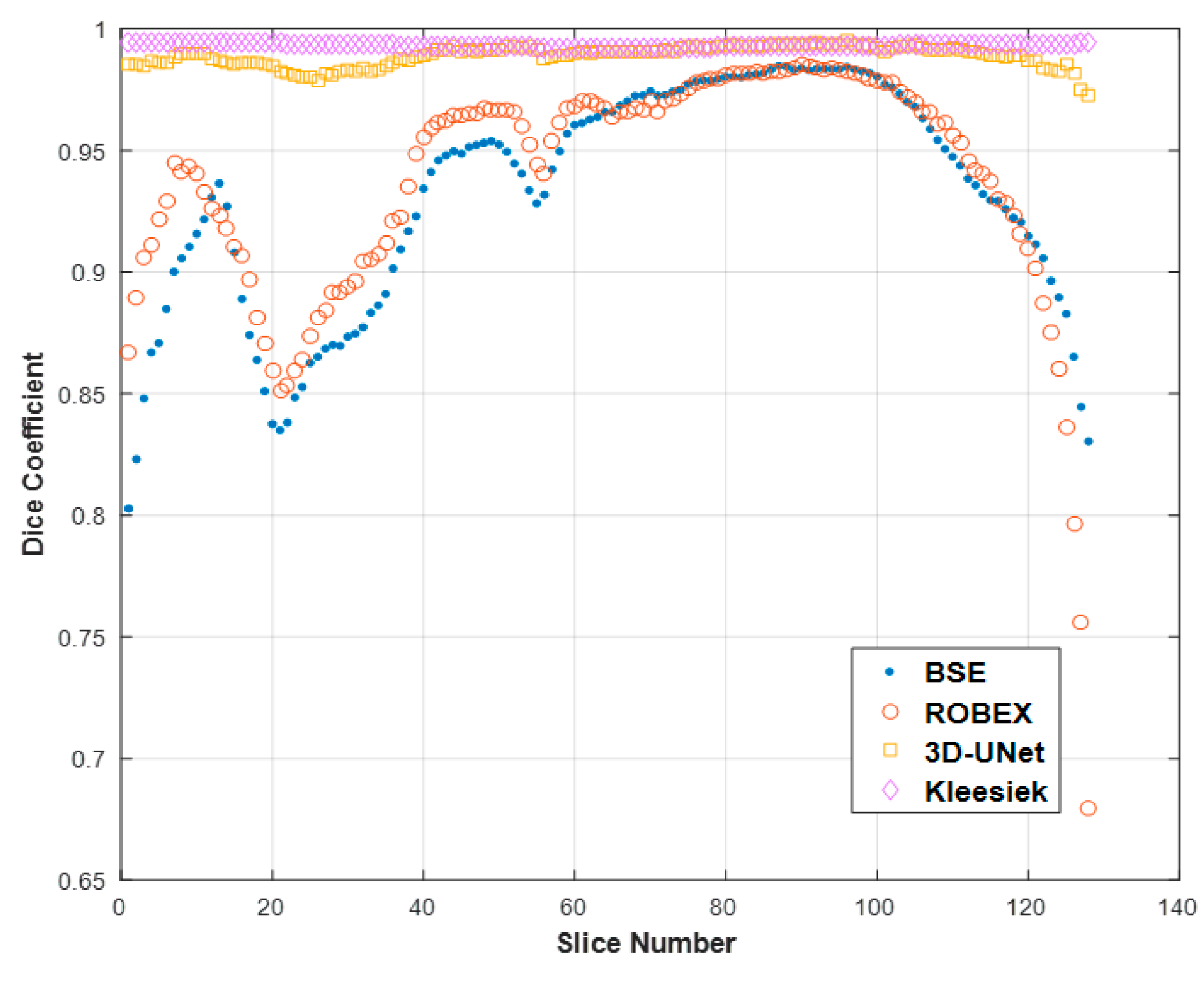
Figure 3.
Dice comparison of 3D-UNet with BSE, ROBEX and Kleesiek’s method on a single test brain MRI scan slice-by-slice. BSE and ROBEX failed to correctly segment the brain in the initial slices of the brain MRI volume. The Dice score in the slices (from 80–140 slices) for both the competitor algorithms is less than 0.90 (on average).

Figure 4.
Skull stripping result on brain image of the eyes. 3D-UNet produced more accurate and smooth segmentation of the brain as compared to BSE and ROBEX. Segmentation failure regions (under or over-segmentation of the brain) are indicated with the rectangles, along with their zoom view.
Figure 4.
Skull stripping result on brain image of the eyes. 3D-UNet produced more accurate and smooth segmentation of the brain as compared to BSE and ROBEX. Segmentation failure regions (under or over-segmentation of the brain) are indicated with the rectangles, along with their zoom view.

Figure 5.
Qualitative performance of the 3D-UNet with BSE and ROBEX. Segmentation failure regions (under or over-segmentation of the brain) are indicated with the rectangles, along with their zoom view.
Figure 5.
Qualitative performance of the 3D-UNet with BSE and ROBEX. Segmentation failure regions (under or over-segmentation of the brain) are indicated with the rectangles, along with their zoom view.

Figure 6.
Qualitative performance comparison of the proposed method. Small rectangles indicate segmentation failure produced by BSE and ROBEX.
Figure 6.
Qualitative performance comparison of the proposed method. Small rectangles indicate segmentation failure produced by BSE and ROBEX.

Figure 7.
Qualitative performance comparison of 3D-UNet with Kleesiek’s method.


Table 1.
3D U-Net architecture.
| Block | Kernel Size | Stride | MaxPool | Activation Function | Batch Norm. | Repeat | Input | Output | Number of Parameters |
|---|---|---|---|---|---|---|---|---|---|
| 1 | 33 | 1 | No | ReLu | Yes | 2 | 643 × 1 | 643 × 48 | 63,504 |
| 2 | 33 | 2 | 33 | - | No | 1 | 643 × 48 | 323 × 48 | - |
| 3 | 33 | 1 | No | ReLu | Yes | 2 | 323 × 48 | 323 × 96 | 373,248 |
| 4 | 33 | 2 | 33 | - | No | 1 | 323 × 96 | 163 × 96 | - |
| 5 | 33 | 1 | No | ReLu | Yes | 2 | 163 × 96 | 163 × 192 | 1,492,992 |
| 6 | 33 | 2 | 33 | - | No | 1 | 163 × 192 | 83 × 192 | - |
| 7 | 33 | 1 | No | ReLu | Yes | 2 | 83 × 192 | 83 × 384 | 5,971,968 |
| 8 | 23 | 2 | No | ReLu | Yes | 1 | 83 × 384 | 163 × (192 + 192) | 1,179,648 |
| 9 | 33 | 1 | No | ReLu | Yes | 2 | 163 × (192 + 192) | 163 × 192 | 2,985,984 |
| 10 | 23 | 2 | No | ReLu | Yes | 1 | 163 × 192 | 323 × (96 + 96) | 294,912 |
| 11 | 33 | 1 | No | ReLu | Yes | 2 | 323 × (96 + 96) | 323 × 96 | 746,496 |
| 12 | 23 | 2 | No | ReLu | Yes | 1 | 323 × 96 | 643 × (48 + 48) | 73,728 |
| 13 | 33 | 1 | No | ReLu | Yes | 2 | 643 × (48 + 48) | 643 × 48 | 186,624 |
| 14 | 13 | 1 | No | SoftMax | No | 1 | 643 × 48 | 643 × 2 | 96 |
| Total number of parameters | 13,369,200 | ||||||||
Table 2.
Overall quantitative analysis and comparison of 3D-UNet with Brain Surface Extractor (BSE) and Robust Brain Extraction (ROBEX) against manual segmentation results for the test brain MRIs datasets. The best values are emboldened.
Table 2.
Overall quantitative analysis and comparison of 3D-UNet with Brain Surface Extractor (BSE) and Robust Brain Extraction (ROBEX) against manual segmentation results for the test brain MRIs datasets. The best values are emboldened.
| Subject I.D. | Dice Coefficient | Sensitivity | Specificity | ||||||
|---|---|---|---|---|---|---|---|---|---|
| BSE | ROBEX | 3D UNet | BSE | ROBEX | 3D UNet | BSE | ROBEX | 3D UNet | |
| A00061276 | 0.9435 | 0.9568 | 0.9908 | 0.8883 | 0.9413 | 0.9853 | 0.9929 | 0.9710 | 0.9962 |
| A00061387 | 0.9547 | 0.9431 | 0.9911 | 0.9186 | 0.9530 | 0.9865 | 0.9876 | 0.9342 | 0.9956 |
| A00061709 | 0.9583 | 0.9528 | 0.9888 | 0.9306 | 0.9512 | 0.9890 | 0.9838 | 0.9543 | 0.9885 |
| A00061711 | 0.9663 | 0.9467 | 0.9896 | 0.9435 | 0.9395 | 0.9856 | 0.9876 | 0.9531 | 0.9935 |
| A00061806 | 0.9637 | 0.8793 | 0.9876 | 0.9313 | 0.8511 | 0.9797 | 0.9939 | 0.9015 | 0.9953 |
| A00062210 | 0.964 | 0.9508 | 0.9913 | 0.9336 | 0.9216 | 0.9891 | 0.9923 | 0.9774 | 0.9934 |
| A00062248 | 0.9585 | 0.9579 | 0.9914 | 0.9208 | 0.9434 | 0.9858 | 0.9933 | 0.9713 | 0.9969 |
| A00062266 | 0.9482 | 0.9546 | 0.9915 | 0.8919 | 0.9521 | 0.9863 | 0.9989 | 0.9569 | 0.9966 |
| A00062282 | 0.9587 | 0.9466 | 0.9897 | 0.9314 | 0.9519 | 0.9826 | 0.9838 | 0.9417 | 0.9967 |
| A00062288 | 0.9674 | 0.9473 | 0.9905 | 0.9438 | 0.9397 | 0.9842 | 0.9895 | 0.9542 | 0.9968 |
| A00062351 | 0.9554 | 0.9488 | 0.9909 | 0.9235 | 0.9328 | 0.9907 | 0.9846 | 0.9633 | 0.9912 |
| A00062917 | 0.9557 | 0.9549 | 0.9897 | 0.9278 | 0.9338 | 0.9839 | 0.9813 | 0.9741 | 0.9954 |
| A00062934 | 0.9197 | 0.9451 | 0.9921 | 0.8329 | 0.9409 | 0.9887 | 0.9935 | 0.9487 | 0.9954 |
| A00062942 | 0.9608 | 0.9507 | 0.9922 | 0.9225 | 0.9164 | 0.9877 | 0.9962 | 0.9817 | 0.9966 |
| A00063008 | 0.9705 | 0.9588 | 0.9915 | 0.9437 | 0.9334 | 0.9883 | 0.9957 | 0.9823 | 0.9947 |
| A00063103 | 0.9544 | 0.9602 | 0.9884 | 0.9116 | 0.9434 | 0.9794 | 0.9935 | 0.9757 | 0.9972 |
| A00063326 | 0.9436 | 0.9503 | 0.9896 | 0.8956 | 0.9372 | 0.9811 | 0.9864 | 0.9621 | 0.9979 |
| A00063368 | 0.953 | 0.9478 | 0.9861 | 0.9030 | 0.9370 | 0.9751 | 0.9985 | 0.9575 | 0.9967 |
| A00063589 | 0.9607 | 0.9512 | 0.9916 | 0.9349 | 0.9440 | 0.9877 | 0.9846 | 0.9577 | 0.9956 |
| A00064081 | 0.9647 | 0.9511 | 0.9923 | 0.9296 | 0.9209 | 0.9888 | 0.9974 | 0.9785 | 0.9958 |
| Mean | 0.9561 | 0.9477 | 0.9903 | 0.9179 | 0.9342 | 0.9853 | 0.9908 | 0.9599 | 0.9953 |
| Standard deviation | 0.0113 | 0.0168 | 0.0016 | 0.0260 | 0.0221 | 0.0040 | 0.0055 | 0.0192 | 0.0022 |
Table 3.
Comparison of mean and standard deviation for J Kleesiek’s method and 3D U-Net. The best values are emboldened.
Table 3.
Comparison of mean and standard deviation for J Kleesiek’s method and 3D U-Net. The best values are emboldened.
| Mean & Standard Deviation | Dice Coefficient | Sensitivity | Specificity | |||
|---|---|---|---|---|---|---|
| Method | J Kleesiek | 3D UNet | J Kleesiek | 3D UNet | J Kleesiek | 3D UNet |
| Mean | 0.9950 | 0.9903 | 0.9745 | 0.9853 | 0.9973 | 0.9953 |
| Std. | 0.0008 | 0.0016 | 0.0063 | 0.0040 | 0.0007 | 0.0022 |
© 2019 by the authors. Licensee MDPI, Basel, Switzerland. This article is an open access article distributed under the terms and conditions of the Creative Commons Attribution (CC BY) license (http://creativecommons.org/licenses/by/4.0/).
Share and Cite
MDPI and ACS Style
Hwang, H.; Rehman, H.Z.U.; Lee, S. 3D U-Net for Skull Stripping in Brain MRI. Appl. Sci. 2019, 9, 569. https://doi.org/10.3390/app9030569
AMA Style
Hwang H, Rehman HZU, Lee S. 3D U-Net for Skull Stripping in Brain MRI. Applied Sciences. 2019; 9(3):569. https://doi.org/10.3390/app9030569
Chicago/Turabian StyleHwang, Hyunho, Hafiz Zia Ur Rehman, and Sungon Lee. 2019. "3D U-Net for Skull Stripping in Brain MRI" Applied Sciences 9, no. 3: 569. https://doi.org/10.3390/app9030569
Note that from the first issue of 2016, this journal uses article numbers instead of page numbers. See further details here.