Development of Multi-Staged Adaptive Filtering Algorithm for Periodic Structure-Based Active Vibration Control System

Abstract

A digital adaptive filtering system is applied to various fields such as current disturbance, noise cancellation, and active vibration and noise control. The least mean squares (LMS) algorithm is widely adopted, owing to its simplicity and low computational burden. A limitation of the LMS algorithm with fixed step size is the trade-off between convergence speed and stability. Several studies have tried to overcome this limitation by varying the step size according to filter input and error; however, the related algorithms with variable step size have not been suitable for signals with complex frequency spectra. As the error decreases, the quality of the output signal deteriorates due to the increase in the higher-order components, depending on the characteristics of the algorithm. Therefore, a novel adaptive filtering algorithm was proposed to overcome these drawbacks. It increased the stability of the system by decreasing the step size using an exponential function. In addition, the error was reduced through normalization using the power of the input signal in the initial state, and the misadjustments in the system were adjusted properly by introducing an energy autocorrelation function of instantaneous error. Furthermore, a novel multi-staged adaptive LMS (MSA-LMS) algorithm was introduced and applied to active periodic structures. The proposed algorithm was validated by simulation and observed to be superior to the conventional LMS algorithms. The results of this study can be applied to active control systems for the reduction of vibration and noise signals with complex spectra in next-generation powertrains, such as hybrid and electric vehicles.

1. Introduction

An adaptive filter adjusts its frequency response automatically according to a predetermined performance criterion. Owing to its self-tuning capability, it has a wide range of applications in signal processing, especially navigation systems (e.g., radar) and biosignal processing. A digital system, such as an adaptive filter, requires an algorithm to update the filter coefficients. The least mean squares (LMS) algorithm was first proposed by Widrow and Hoff [1] in the 1960s as a representative algorithm. This algorithm is flexible, robust, and easy to implement; however, it has a limitation with respect to the trade-off between convergence speed and stability: (1) The system is likely to become unstable with a rapidly changing disturbance when the related parameters are adjusted to increase the convergence speed of the control filter; (2) the convergence speed is lowered when the parameters are adjusted to increase the stability.

Many research efforts have helped enhance LMS algorithms by suitable control of the step size to resolve the issue of trade-off between convergence speed and stability. The normalized LMS (NLMS) algorithm was developed to overcome this limitation by normalizing the input value with an autocorrelation function [2]. The variable step-size LMS algorithm (VS-LMS) uses a modified sigmoid function to introduce a new step size with tracking error [3]. A variable-parameter algorithm has been developed in which the step size is determined using the sum of two exponential functions, their coefficients, and the weight ratio of the output error [4]. A modified LMS (MLMS) algorithm with a modified step size, in which the product of filter input and error is used as an exponential decay parameter, has also been developed [5]. Step size is also adjusted by using the linear sum of the step size and error value square of the immediately preceding step. This includes the constraints of the step size range and reduces the sensitivity to misadjustment in a stable or unstable environment [6]. A stochastic gradient adaptive filter with step size varied, using an autocorrelation function of the error has also been developed [7]. A robust adaptive algorithm was developed by using autocorrelation functions of errors, regardless of the presence of disturbances (e.g., noise) [8]. Another adaptive algorithm, developed to effectively cancel the echo of the hands-free telephone, helps estimate the power of an unmeasurable signal using various detection techniques and to derive the optimum step size to make the system faster and more reliable [9]. There are several VS-LMS algorithms, but with increased computation time [10]. Finally, a variable step-size algorithm including filter error, filter input, and an affine projection algorithm has been proposed to realize faster convergence and smaller misadjustments [11].

However, there is little research on achieving stability and rapid convergence in the case of signals with complex frequency spectra, and therefore, a careful analysis of the signal tracking performance depending on the type of signal is needed. Next-generation powertrains, such as electric cars and hybrid cars, exhibit vibration and noise signals with complex spectra associated with motors and gearboxes. However, attenuation of passive vibration through structural changes is significantly limited, and therefore, active control systems and algorithms with new concepts are needed for reduction of vibration and noise.

This study proposes a new active vibration control system and a multi-staged adaptive algorithm for attenuating signals with complex frequency spectra systematically. The performance of the proposed algorithm is validated with the simulation of two different signals, incommensurate sinusoids and periodic sinusoids, and is compared with the existing algorithm. Furthermore, the applicability of the proposed algorithm to practical systems is discussed. The composition of this paper is as follows: Section 2 describes the existing LMS adaptive algorithm. Section 3 explains the new concept of step size applied to the MSA-LMS adaptive filter. Section 4 analyzes the new adaptive filter with the MSA-LMS algorithm. Finally, Section 5 draws conclusions and discusses future plans.

2. Least Mean Squares Algorithm

An adaptive digital filtering system is generally used for active control of noise and vibration. The least mean squares (LMS) used in the system shown in Figure 1 below is the most commonly used feedforward algorithm [12].

The formula for updating the weights of an LMS algorithm is defined as

$$\begin{array}{l}w(k+1)=w(k)+1/2\cdot \mu \left[-\nabla \right]\\ \hspace{1em}\hspace{1em}\hspace{1em} =w(k)+\mu \cdot \left[x^T(k)\cdot d(k)-x(k)\cdot x^T(k)\cdot w(k)\right]\\ \hspace{1em}\hspace{1em}\hspace{1em} =w(k)+\mu \cdot \left[x^T(k)\cdot (d(k)-x(k)\cdot w(k))\right]\\ \hspace{1em}\hspace{1em}\hspace{1em} =w(k)+\mu \cdot x^T(k)\cdot e(k)\end{array}$$

(1)

Here, $\mu$ is a factor that determines the convergence speed of an LMS algorithm. It is referred to as step size and is related to the update of the weights. When $\mu$ is relatively small, it takes a long time to find the weight that minimizes the slope of the squared error curve because the change in the weight is small at each sampling time. However, when $\mu$ is relatively large, the control system becomes unstable and fails to find the correct value. Therefore, $\mu$ is critical to the performance of an LMS algorithm. The range of $\mu$ for the convergence of an LMS algorithm is as follows, where ${\lambda }_{\max }$ is the maximum eigenvalue of the autocorrelation matrix consisting of input signal $x(k)$.

$$0<\mu <\frac{1}{{\lambda }_{\max }}$$

(2)

As described above, an LMS adaptive filter involves simple calculations. However, since the convergence speed is relatively less, it takes a long time to approach the optimum filter coefficient. In addition, the convergence characteristic is very dynamic. Particularly, since the step size is fixed, a drastic change in the target signal cannot be tracked properly. To overcome these limitations, several adaptive filter algorithms with variable step size have been studied recently. Most of these algorithms use variable steps represented by complex expressions, and therefore require extensive computations, although they use optimal step size to adapt to the magnitude and direction of the target signal. For example, when the response signal of the system changes greatly as a transient state at the beginning of a signal input to the system, a relatively large step size is applied. After a certain time, the weight of the adaptive filter becomes an optimal value, the error signal becomes smaller, and consequently, the step size becomes relatively small. Finally, in the steady state, the error value becomes close to 0, and the step size can be used as a fixed value without a large change.

3. MSA-LMS Adaptive Filter

3.1. Step Size of MSA-LMS Adaptive Filter

The size of input signal power affects the performance of an algorithm. Therefore, a strong input signal power requires a relatively large step size. In this case, stable values cannot be found frequently in the steady state. Conversely, a weak input signal power requires a relatively small step size and, consequently, convergence is slowed down.

In this study, the step size is first divided into an autocorrelation matrix of input signal power as shown in the following equation, and it is changed according to signal size.

$$\frac{1}{[u(k)u(k-1)]{[u(k)u(k-1)]}^T}$$

(3)

In the case of a general adaptive filter, the larger the step size is, the faster the convergence can be. The step size normalized by the input signal power changes according to the input power and does not diverge. In addition, it facilitates much faster convergence compared with a general algorithm.

Second, to achieve convergence with a large step size in the initial stage and to obtain good stability in the steady state, an exponential function as follows is introduced to converge to a small value.

$$e^{-\gamma \cdot \left|e(k)\cdot e(k-1)\right|}$$

(4)

Finally, an autocorrelation function of the instantaneous error is used so that adjustment of a misadjustment is not needed. Because the power of the error is large, the parameter $\gamma$ can control the convergence time as well as adjust the misadjustments.

$$\gamma \cdot e(k)\cdot e(k-1)$$

(5)

Instead of fixed LMS step size, $\gamma$ can be adjusted to vary the step size and thereby improve the algorithm in respect to both robustness and flexibility. The optimal step size is achieved by adjusting A $(0<A<1)$, B $(0<B<1)$, and C $(0<C<1)$ in the expression as follows:

$$\mu =\frac{A}{[u(k)u(k-1)]{[u(k)u(k-1)]}^T[B\cdot \mu (k-1)+C\cdot e^{-\gamma \cdot \left|e(k)\cdot e(k-1)\right|}]}$$

(6)

3.2. MSA-LMS Adaptive Filter Implementation and Analysis

An adaptive filter updates the coefficient of the filter or the system parameters automatically by an adaptive algorithm so that the system reaches the optimum state.

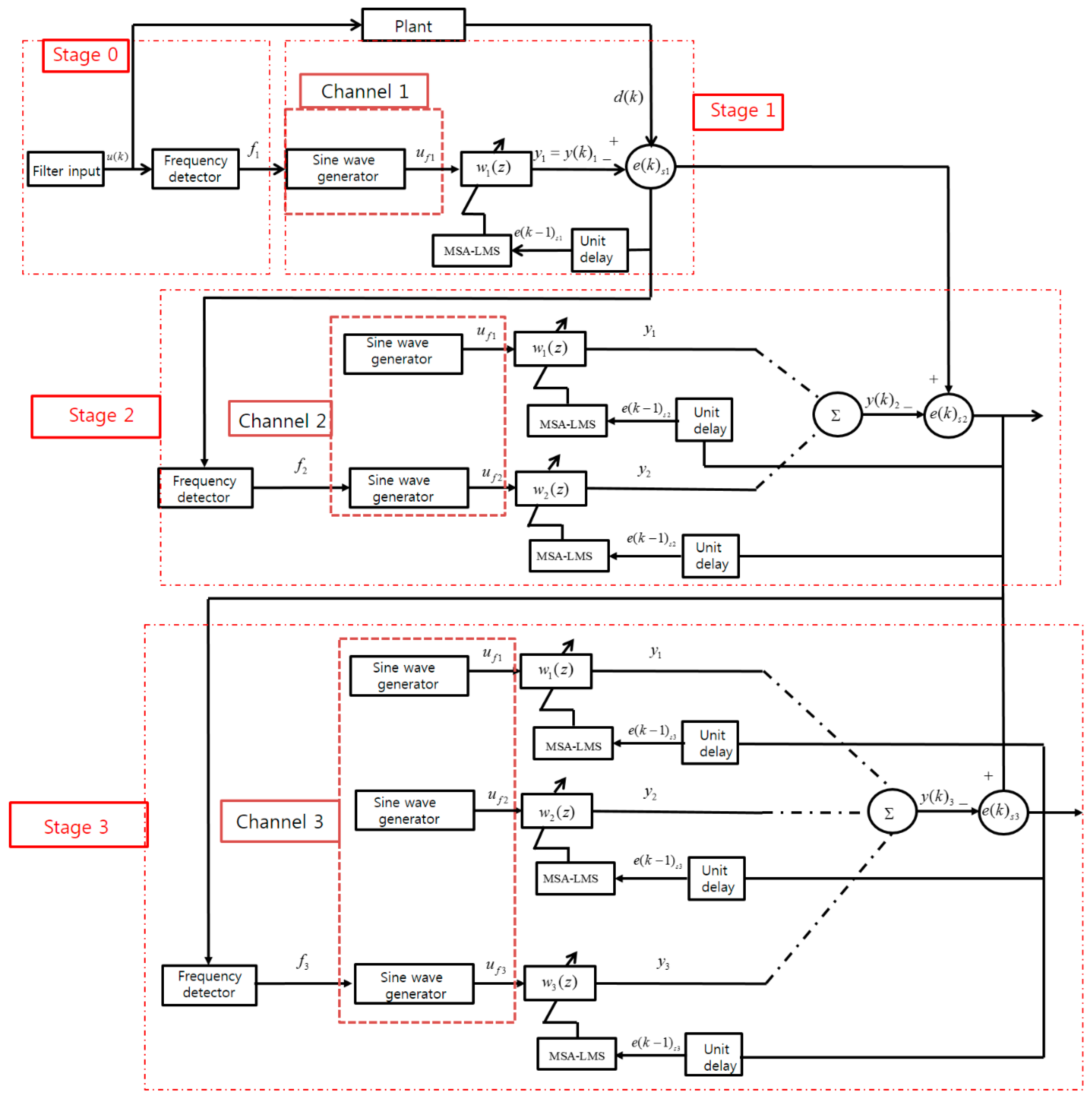
Adaptive filters are widely used in various fields of communication-signal processing, such as radar and active control of vibration and noise, owing to their self-tuning ability to change the signal to be tracked and the surrounding situation. The structure of the proposed MSA-LMS adaptive filter is shown in Figure 2.

The proposed algorithm is verified by simulation for four types of signals: “Incommensurate Sinusoids”, “Periodic Sinusoids”, “Beating”, and “Amplitude Modulated”. The vibration reduction performance is found to be much improved. This result can be applied to an active control system for the reduction of vibration and noise in a next-generation powertrain; for example, it has recently been applied to an electric car having signals with complex spectra. The MSA-LMS algorithm is implemented in four stages: Stage 0, Stage 1, Stage 2, and Stage 3. If the same algorithm is used in the control system of each stage of the active period structure, improvement of tracking performance will not be expected regardless of the stage. Therefore, we proposed the above structure to allow a different control for each stage. Based on the MSA-LMS algorithm, Stage 1 is applied to active element 1 of an active control system, Stage 2 to active element 2, and Stage 3 to active element 3. As the stage increases, the number of channels of the adaptive filter is increased, and the frequency of the resultant signal of the LMS algorithm is additionally targeted to improve the tracking performance and minimize the error value.

In the simulation performed in this study, the control time of the four stages is set as 1 s, and the sampling time is defined as 0.0001 s. Accordingly, Stage 0 has a range from 0 to 0.9999 s, Stage 1 from 1 to 1.9999 s, Stage 2 from 2 to 2.9999 s, and Stage 3 from 3 to 3.9999 s.

3.2.1. Stage 0

Stage 0 has a frequency detector. There are various methods of frequency estimation using a digital signal processor (DSP). The frequency is estimated by counting the number of times $C$ a given signal crosses the x-axis in one cycle of period $T$ through a detector, and then by substituting $T$ and $C$ into the equation below. The process can be illustrated by Figure 3 [13].

$$f=\frac{1}{2CT}$$

(7)

The input signal $u(k)$ passes through the zero-crossing detector, and the number of times $C$ the input signal crosses the x-axis is indicated by the counter. The frequency $f_1$ of the input signal can then be estimated from 0 to 0.9999 s as explained above.

3.2.2. Stage 1

In Stage 1, the output of a general adaptive filter is obtained by multiplying the input signal by the filter weight. In contrast, the input signal $u_{f_1}$ of the proposed adaptive filter is the output of the sine wave generator at the frequency $f_1$ (measured from Stage 0) in the range of 1 to 1.9999 s, and is expressed as below:

$$u_{f1}=\sin (2\cdot \pi \cdot f_1\cdot t_2)$$

(8)

Since only the filter output signal $y_1$ is present, it is the same as the total output signal $y{(k)}_1$ and can be expressed as:

$$y_1=y{(k)}_1=u_{f1}\cdot w_1^T={u_{f1}}^T\cdot w_1$$

(9)

The desired signal response and the error of the filter output signal are expressed as follows:

$$e{(k)}_{s1}=d(k)-y{(k)}_1=d(k)-u_{f1}\cdot w_1^T=d(k)-{u_{f1}}^T\cdot w_1$$

(10)

The $e{(k-1)}_{s1}$ signal is applied one step before the error signal $e{(k)}_{s1}$ to the MSA-LMS algorithm and is updated repeatedly.

3.2.3. Stage 2

The error signal $e{(k)}_{s1}$ is an unknown signal and cannot be measured. The frequency $f_2$ of the error signal $e{(k)}_{s1}$ is estimated from the number of times $C$ the signal passes through the x-axis as sensed by the zero-crossing detector and indicated by the counter. Using the output of the sine wave generator at the estimated $f_2$, the function $u_{f2}$ between 2 and 2.9999 s is expressed as follows:

$$u_{f2}=0.5\cdot \sin (2\cdot \pi \cdot f_2\cdot t_2)$$

(11)

To avoid the amplitude of the input signal from increasing with the update of the filter coefficients, the signal is multiplied by 0.5. Thus, in Stage 2, the following signal appears additionally:

$$u_{f1}=0.5\cdot \sin (2\cdot \pi \cdot f_1\cdot t_2)$$

(12)

Therefore, the filter output of Stage 2 appears as follows,

$$\begin{array}{l}{u}_{f1}=0.5\cdot \sin (2\cdot \pi \cdot f_1\cdot t_2)\\ u_{f2}=0.5\cdot \sin (2\cdot \pi \cdot f_2\cdot t_2)\end{array}$$

(13)

The output signal $y_2$ is expressed as

$$y_2=u_{f2}\cdot w_2^T={u_{f2}}^T\cdot w_2$$

(14)

Since there are two input signals in Stage 2, the total output signal of the filter $y{(k)}_2$ appears as follows:

$$\begin{array}{l}y{(k)}_2=y_1+y_2=u_{f1}\\ \hspace{0.17em}\hspace{0.17em}\hspace{0.17em}\hspace{0.17em}\hspace{0.17em}\hspace{0.17em}\hspace{0.17em}=0.5\sin (2\cdot \pi \cdot f_1\cdot t_2)\cdot w_1+0.5\sin (2\cdot \pi \cdot f_2\cdot t_2)\cdot w_2\end{array}$$

(15)

In Stage 1, the error signal $e{(k)}_{s1}$ is the $d(k)$ of Stage 2. The filter output $y{(k)}_2$ and error signal are expressed as follows:

$$\begin{array}{l}e{(k)}_{s2}=e{(k)}_{s1}-y{(k)}_2\\ \hspace{0.17em}\hspace{0.17em}\hspace{0.17em}\hspace{0.17em}\hspace{0.17em}\hspace{0.17em}\hspace{0.17em}\hspace{0.17em}=e{(k)}_{s1}-u_{f1}\cdot w_1^T-u_{f2}\cdot w_2^T\\ \hspace{0.17em}\hspace{0.17em}\hspace{0.17em}\hspace{0.17em}\hspace{0.17em}\hspace{0.17em}\hspace{0.17em}\hspace{0.17em}=e{(k)}_{s1}-{u_{f1}}^T\cdot w_1-{u_{f2}}^T\cdot w_2\end{array}$$

(16)

The $e{(k-1)}_{s2}$ signal is applied one step before the error signal $e{(k)}_{s2}$ to the MSA-LMS algorithm and is updated repeatedly.

3.2.4. Stage 3

The error signal $e{(k)}_{s2}$ is an unknown signal and cannot be measured. The frequency $f_3$ of the error signal $e{(k)}_{s2}$ is estimated from the number of times $C$ the signal passes through the x-axis, as sensed by the zero-crossing detector and indicated by the counter. Using the output of the sine wave generator at the estimated frequency $f_3$, the function $u_{f3}$ between 3 and 3.9999 s is expressed as follows:

$$u_{f3}=1/3\cdot \sin (2\cdot \pi \cdot f_3\cdot t_2)$$

(17)

The signal is multiplied by $1/3$ to avoid the amplitude of the input signal from increasing as the filter coefficient is updated. Thus, in Stage 3, the following signals appear additionally:

$$\begin{array}{l}{u}_{f1}=1/3\cdot \sin (2\cdot \pi \cdot f_1\cdot t_2)\\ u_{f2}=1/3\cdot \sin (2\cdot \pi \cdot f_2\cdot t_2)\end{array}$$

(18)

Therefore, the filter output of Stage 3 appears as follows,

$$\begin{array}{l}{u}_{f1}=1/3\cdot \sin (2\cdot \pi \cdot f_1\cdot t_2)\\ u_{f2}=1/3\cdot \sin (2\cdot \pi \cdot f_2\cdot t_2)\\ u_{f3}=1/3\cdot \sin (2\cdot \pi \cdot f_3\cdot t_2)\end{array}$$

(19)

The total filter output signal $y_3$ is shown as

$$y_3=u_{f3}\cdot w_3^T={u_{f3}}^T\cdot w_3$$

(20)

Since there are three input signals in Stage 3, the total output signal of the filter $y{(k)}_3$ appears as follows:

$$\begin{array}{l}y{(k)}_3=y_1+y_2+y_3\\ \hspace{0.17em}\hspace{0.17em}\hspace{0.17em}\hspace{0.17em}\hspace{0.17em}\hspace{0.17em}\hspace{0.17em}\hspace{0.17em}=1/3\cdot \sin (2\cdot \pi \cdot f_1\cdot t_2)\cdot w_1^T+1/3\cdot \sin (2\cdot \pi \cdot f_2\cdot t_2)\cdot w_2^T\\ \hspace{0.17em}\hspace{0.17em}\hspace{0.17em}\hspace{0.17em}\hspace{0.17em}\hspace{0.17em}\hspace{0.17em}\hspace{0.17em}\hspace{0.17em}\hspace{0.17em}\hspace{0.17em}\hspace{0.17em}\hspace{0.17em}\hspace{0.17em}\hspace{0.17em}+1/3\cdot \sin (2\cdot \pi \cdot f_3\cdot t_2)\cdot w_3^T\end{array}$$

(21)

In Stage 2, the error signal $e{(k)}_{s2}$ is $d(k)$ of Stage 3. The filter output $y{(k)}_3$ and error signal $e{(k)}_{s3}$ are expressed as follows:

$$e{(k)}_{s3}=e{(k)}_{s2}-y{(k)}_3$$

(22)

The $e{(k-1)}_{s3}$ signal is applied one step before the error signal $e{(k)}_{s3}$ to the MSA-LMS algorithm and is updated repeatedly.

4. Simulation

To verify the performance of the MSA-LMS algorithm proposed in this study, an active control system based on the active periodic structure for reduction or elimination of undesired vibration and noise signals was simulated. Although there were various multi-frequency vibration signals, we verified the control performance for general quasi-periodic signals, not limited to special cases such as modulation signals. Incommensurate sinusoids were represented by the following equations and they were classified according to the amplitude, frequency, and phase [14]:

$$x(t)=A_1\sin ({\omega }_{1}t+{\theta }_1)+A_2\sin ({\omega }_{2}t+{\theta }_2)+A_3\sin ({\omega }_{3}t+{\theta }_3)$$

(23)

where $A_i$ is the amplitude, ${\omega }_i$ is the frequency, and ${\theta }_i$ is the phase. The existing LMS algorithm had a limited performance for a complex frequency spectrum. Furthermore, the error increased with the size of the input signal and the misadjustment was due to the initial value. As a result, the wideband frequency component, according to the algorithm characteristics, deteriorated, and the output signal in the time domain became noisy. The MSA-LMS algorithm was proposed to overcome these limitations, and the performance of the algorithm was verified for two types of signals: “Periodic Sinusoids” and “Incommensurate Sinusoids”.

4.1. Periodic Sinusoids: ${\omega }_{2,3}=n{\omega }_1$

For periodic sinusoids, we used $A_1=0.02$, $A_2=0.05$, $A_3=0.03$, ${\omega }_1=10 \mathrm{Hz}$, ${\omega }_2=30 \mathrm{Hz}$, and ${\omega }_3=40 \mathrm{Hz}$. It was assumed that there was no phase difference in each term.

Figure 4 is a graph comparing the signal tracking performance between the LMS algorithm and the proposed MSA-LMS algorithm. It can be seen that the MSA-LMS algorithm with step-size changing for each sampling time according to exponential and autocorrelation functions was superior to the LMS algorithm with fixed step size over the entire simulation range of time.

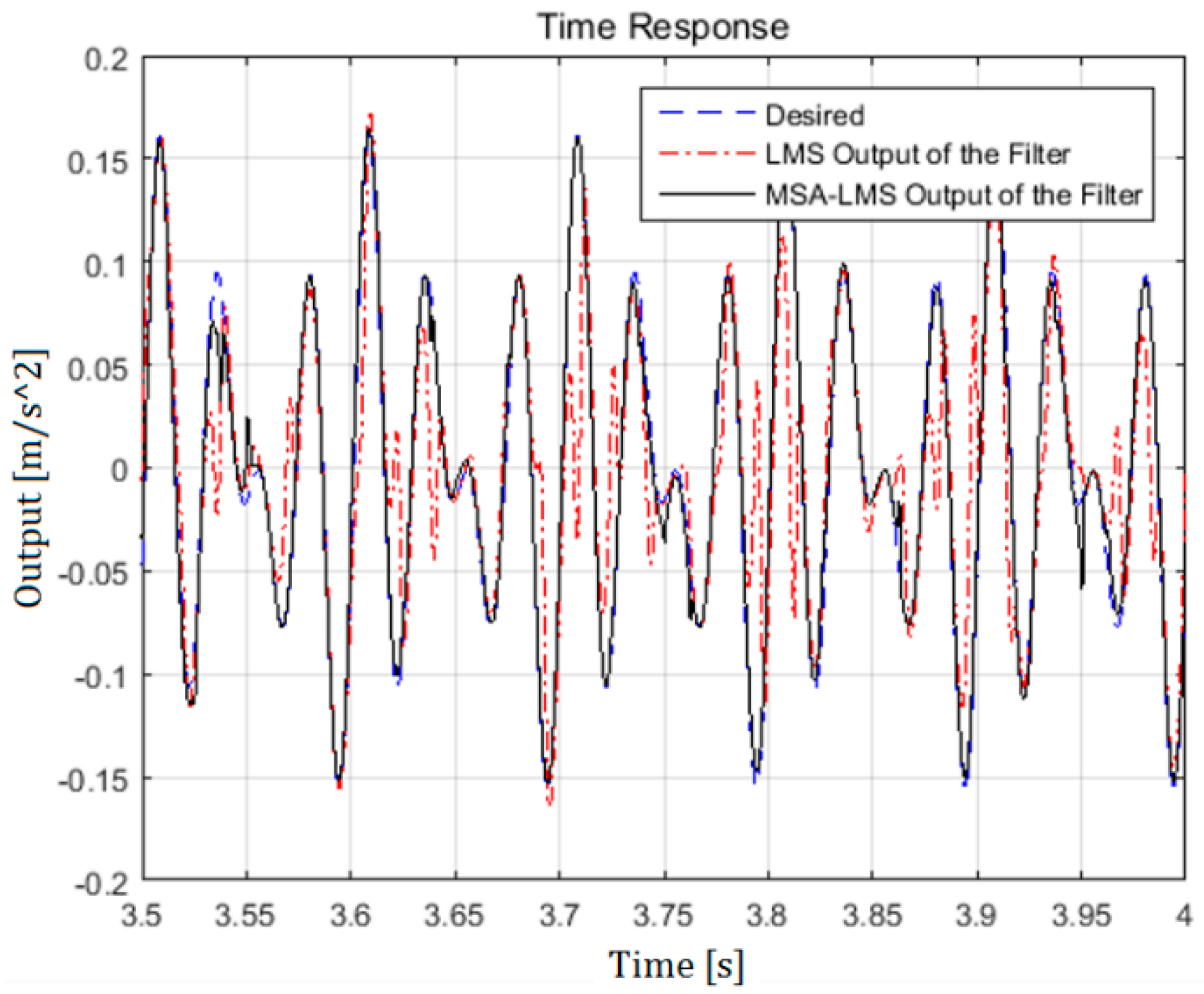
To compare the tracking performance between the LMS algorithm and the proposed MSA-LMS algorithm in detail, the interval from 3.5 to 4 s was enlarged, as shown in Figure 5. In the case of the LMS algorithm, it can be observed that the tracking performance for the desired signal was significantly lowered from the second-high peak to the low peak near 3.55 s. Furthermore, the direction was completely reversed in the middle of a vibration signal, which may have caused a spillover phenomenon with a higher frequency component than the original signal. On the other hand, in the case of the MSA-LMS algorithm using an energy autocorrelation function of instantaneous error, the misadjustment was found to be properly adjusted and the tracking performance was excellent.

Figure 6 compares the estimation error of the active vibration control between the two algorithms. It can be observed that both algorithms exhibited almost the same values of error up to 2 s. However, between 2 and 3 s, the maximum and minimum values of the control error were 0.1963 and −0.1915, respectively, for the LMS algorithm, while 0.1176 and −0.1456 for the MSA-LMS algorithm. Similarly, between 3 and 3.5 s, the respective values were 0.1941 and −0.1917 for LMS, while 0.0928 and −0.0622 for MSA-LMS. Finally, between 3.5 and 4 s, the respective values were 0.1930 and 0.1946 for LMS, while 0.0558 and 0.0393 for MSA-LMS.

Based on the above results, the peak-to-peak value of the proposed MSA-LMS algorithm was found to be 32% less than that of the LMS algorithm with fixed step size between 2 and 3 s, 60% less between 3 and 3.5 s, and 75% less between 3.5 and 4 s. However, it may be noted that the peak-to-peak value of the error did not reduce over time for the LMS algorithm, while it gradually reduced for the MSA-LMS algorithm, owing to its adaptability associated with the multi-stage concept. The above results are summarized in

Table 1. Peak-to-Peak value analysis for the estimation errors (“Periodic Sinusoids” case).

Control Algorithm	Error Analysis	Time
		2.0–3.0 s	3.0–3.5 s	3.5–4.0 s
LMS Algorithm	Maximum	0.1963	0.1941	0.1930
	Minimum	−0.1915	−0.1917	−0.1946
	Peak-to-Peak	0.3878	0.3858	0.3876
MSA-LMS Algorithm	Maximum	0.1176	0.0928	0.0558
	Minimum	−0.1456	−0.0622	−0.0393
	Peak-to-Peak	0.2632 (32%↓)	0.1550 (60%↓)	0.0951 (75%↓)

below.

Figure 7 is a graph comparing the error between the LMS algorithm and the proposed MSA-LMS algorithm. Since the MSA-LMS algorithm had an energy autocorrelation function of exponential function and instantaneous error, it can be seen that the error gradually decreased from 2 s onwards, while no such reduction was observed in the case of the LMS algorithm.

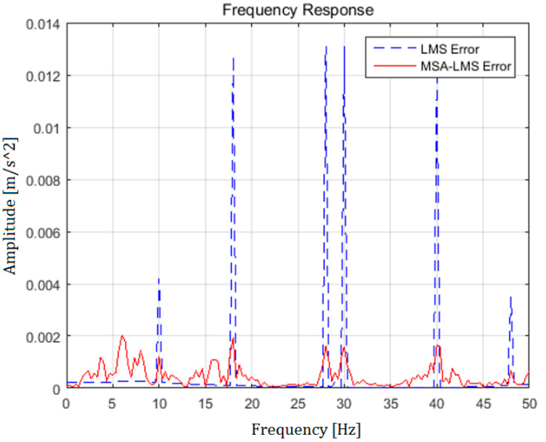
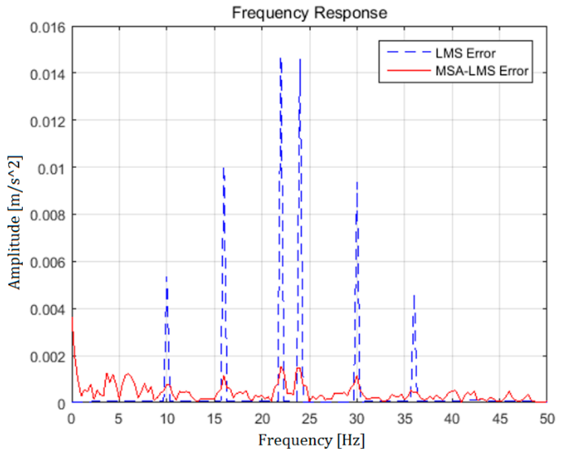
Figure 8 is a graph comparing the frequency spectra of the proposed MSA-LMS algorithm with the LMS algorithm. The main peaks at $w_1=10 \mathrm{Hz}$, $w_2=30 \mathrm{Hz}$, and $w_3=40 \mathrm{Hz}$ for the MSA-LMS algorithm were reduced by 5 to 9 dB, compared with the LMS algorithm. However, in the case of the MSA-LMS algorithm, the spillover phenomenon in the broadband was slightly increased. It is thought that this phenomenon occurs as the frequency component increases with the stage, and is attributed to the characteristics of the multi-stage structure of the algorithm.

At a point $k$, when the conventional LMS algorithm was applied to four incommensurate sinusoids, there was an unexpected frequency other than the frequency component of the input signal, due to the unintentional modulation process between filter input $x[k]$ and error $e[k]$. Some were observed. This frequency component can be confirmed by analyzing the $x[k]\cdot e[k]$ as follows: In all cases, the frequency of the reference signal is assumed to be ${\omega }_2$, the phase difference. The frequency components at the first sampling point $k=1$ are as follows:

$$x[k]\cdot e[k]=\cos ({\omega }_{2}t)\cdot \left\{\cos ({\omega }_{1}t)+\cos ({\omega }_{2}t)+\cos ({\omega }_{3}t)\right\}$$

(24)

$$\begin{array}{l}y\left[x[k]\cdot e[k]\right]=\frac{1}{2}\pi \left[\delta (\omega +{\omega }_1-{\omega }_2)+\delta (\omega -{\omega }_1-{\omega }_2)\right]\\ \hspace{0.17em}\hspace{0.17em}\hspace{0.17em}\hspace{0.17em}\hspace{0.17em}\hspace{0.17em}\hspace{0.17em}\hspace{0.17em}\hspace{0.17em}\hspace{0.17em}\hspace{0.17em}\hspace{0.17em}\hspace{0.17em}\hspace{0.17em}\hspace{0.17em}\hspace{0.17em}\hspace{0.17em}\hspace{0.17em}\hspace{0.17em}+\frac{1}{2}\pi \left[\delta (\omega -{\omega }_3+{\omega }_2)+\delta (\omega -{\omega }_3-{\omega }_2)\right]+\frac{1}{2}\pi \left[\delta (\omega -2{\omega }_2)+\delta (\omega )\right]\end{array}$$

(25)

where $y[]$ is the Fourier transform and Dirac delta function. At the second sampling point $k\ge 2$, the effect of the reference input was added. The frequency components are summarized as follows:

$$\begin{array}{l}x[k]\cdot \left(\left[x[k]\cdot e[k]\right]\right)\\ \hspace{0.17em}\hspace{0.17em}=\cos ({\omega }_{2}t)\cdot \left(\cos ({\omega }_{2}t)\cdot \left\{\cos ({\omega }_{1}t)+\cos ({\omega }_{2}t)+\cos ({\omega }_{3}t)\right\}\right)\end{array}$$

(26)

$$\begin{array}{l}y\left[x[k]\cdot \left(\left[x[k]\cdot e[k]\right]\right)\right]=\frac{1}{4}\pi \left[\delta (\omega +{\omega }_1-2{\omega }_2)+\delta (\omega -{\omega }_1-2{\omega }_2)+2\delta (\omega -{\omega }_1)\right]\\ \hspace{0.17em}\hspace{0.17em}\hspace{0.17em}\hspace{0.17em}\hspace{0.17em}\hspace{0.17em}\hspace{0.17em}\hspace{0.17em}\hspace{0.17em}\hspace{0.17em}\hspace{0.17em}\hspace{0.17em}\hspace{0.17em}\hspace{0.17em}\hspace{0.17em}\hspace{0.17em}\hspace{0.17em}\hspace{0.17em}\hspace{0.17em}\hspace{0.17em}\hspace{0.17em}\hspace{0.17em}\hspace{0.17em}\hspace{0.17em}\hspace{0.17em}\hspace{0.17em}\hspace{0.17em}+\frac{1}{4}\pi \left[\delta (\omega +{\omega }_3-2{\omega }_2)+\delta (\omega -{\omega }_3-2{\omega }_2)+2\delta (\omega -{\omega }_3)\right]\\ \hspace{0.17em}\hspace{0.17em}\hspace{0.17em}\hspace{0.17em}\hspace{0.17em}\hspace{0.17em}\hspace{0.17em}\hspace{0.17em}\hspace{0.17em}\hspace{0.17em}\hspace{0.17em}\hspace{0.17em}\hspace{0.17em}\hspace{0.17em}\hspace{0.17em}\hspace{0.17em}\hspace{0.17em}\hspace{0.17em}\hspace{0.17em}\hspace{0.17em}\hspace{0.17em}\hspace{0.17em}\hspace{0.17em}\hspace{0.17em}\hspace{0.17em}\hspace{0.17em}\hspace{0.17em}+\frac{1}{2}\pi \delta (\omega )+\frac{1}{4}\pi \left[\delta (\omega -{\omega }_2)+\delta (\omega -2{\omega }_3)\right]\end{array}$$

(27)

As can be seen in Equations (25) and (27), the controlled signal includes additional frequency components, such as ${\omega }_j={\omega }_2\pm {\omega }_1$, ${\omega }_3\pm {\omega }_2$, $2{\omega }_2$, $3{\omega }_2$, $2{\omega }_2\pm {\omega }_1$, $2{\omega }_2\pm {\omega }_3$, and so on, ${\omega }_i={\omega }_1$, $2{\omega }_2$, ${\omega }_3$, which were previously included in the control signal. It is also apparent that additional side bands are located at $\Delta {\omega }_a={\omega }_2-{\omega }_1$, $\Delta {\omega }_b={\omega }_3-{\omega }_2$, and $\left|\Delta {\omega }_a-\Delta {\omega }_b\right|$. It can be observed from Figure 8 that these additional frequency components occurred at $\left|2{\omega }_2-{\omega }_1\right|/2\pi =48 \mathrm{Hz}$ and $\left|{\omega }_2-{\omega }_1\right|/2\pi =18 \mathrm{Hz}$. Here, it is determined that the error $2 \mathrm{Hz}$ occurred because the object to be controlled was not the input signal but the response of the secondary system, and the main frequency component of the signal was an estimated value rather than an actual value (presumed to be a nearby value).

4.2. Incommensurate Sinusoids: ${\omega }_2\ne n{\omega }_1,{\omega }_3\ne n{\omega }_1$

For incommensurate sinusoids, $A_1=0.029$, $A_2=0.053$, $A_3=0.071$, ${\omega }_1=10 \mathrm{Hz}$, ${\omega }_2=10 \mathrm{Hz}$, and ${\omega }_2=10 \mathrm{Hz}$ were used as controls. It was also assumed that there was no phase difference in each term.

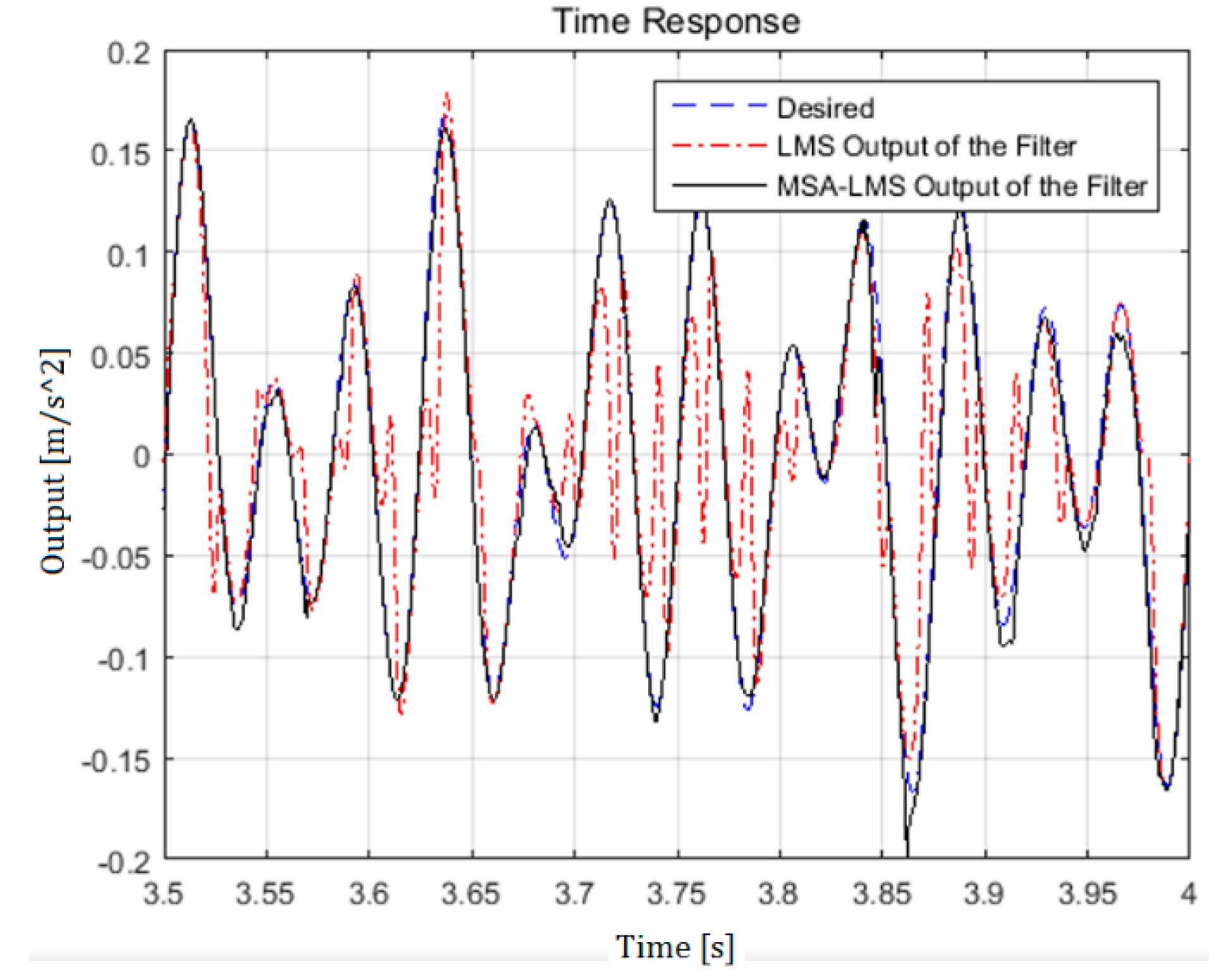
Figure 9 is a graphical comparison between the LMS algorithm and the proposed MSA-LMS algorithm. In the case of “Incommensurate Sinusoids” that were relatively less related to the frequencies involved than the “Periodic Sinusoids” discussed earlier, the signal pattern in the time domain was found to be irregular, as shown in Figure 10. Nevertheless, it can be seen that the signal tracking performance of the proposed MSA-LMS algorithm was much better than that of the LMS algorithm with fixed step size.

To compare the proposed MSA-LMS algorithm with the LMS algorithm in detail, the range from 3.5 to 4 s was expanded, as shown in Figure 10. The MSA-LMS algorithm was adaptive with respect to the frequency and error of the filtered signal. On the other hand, the LMS algorithm that had a fixed step size exhibited a relatively low tracking performance, owing to its failure to detect such changes.

Figure 11 compares the estimation error of the active vibration control between the two algorithms. It can be observed that there was no significant difference up to 2 s. However, between 2 and 3 s, the maximum and minimum values of the control error were 0.1712 and −0.1835, respectively, for the LMS algorithm, while the corresponding values were 0.1305 and −0.059 for the MSA-LMS algorithm. Similarly, between 3 and 3.5 s, the respective values were 0.1701 and −0.1839 for LMS, while 0.0453 and −0.0178 for MSA-LMS. Finally, between 3.5 and 4 s, the respective values were 0.1712 and −0.1858 for LMS, while 0.0651 and −0.0199 for MSA-LMS.

It can be observed from the above results that the peak-to-peak value of the proposed MSA-LMS algorithm, which is more adaptive than the existing LMS algorithm, decreased by 47% between 2 and 3 s, by 82% between 3 and 3.5 s, and by 78% between 3.5 and 4 s. Similar to the previous case (Period Sinusoids), the peak-to-peak value of the error did not decrease over time in the case of the LMS algorithm, whereas it was reduced by about two times in the case of the MSA-LMS algorithm, owing to its multi-stage concept. Because of the complexity of the incommensurate sinusoids, the tracking performance of the LMS algorithm was found to be worse than that observed in the case of the periodic sinusoids, whereas the MSA-LMS algorithm had a similar tracking performance with a higher percentage of decrease in the error value. Figure 12 is a graph comparing the error between the LMS algorithm and the proposed MSA-LMS algorithm. It can be observed that the MSA-LMS algorithm exhibited slightly better tracking performance than that observed in the previous case (Periodic Sinusoids) between 2 and 3 s, by virtue of its energy autocorrelation function of exponential function and instantaneous error. The above results are summarized in

Table 2. Peak-to-Peak value analysis for the estimation errors with LMS and MSA-LMS algorithms (“Incommensurate Sinusoids” case).

Control Algorithm	Error Analysis	Time
		2.0–3.0 s	3.0–3.5 s	3.5–4.0 s
LMS Algorithm	Maximum	0.1712	0.1701	0.1712
	Minimum	−0.1835	−0.1839	−0.1858
	Peak-to-Peak	0.3547	0.3540	0.3876
MSA-LMS Algorithm	Maximum	0.1305	0.0453	0.0651
	Minimum	−0.0590	−0.0178	−0.0199
	Peak-to-Peak	0.1895 (47%↓)	0.0631 (82%↓)	0.0850 (78%↓)

below.

Figure 13 is a graph comparing the frequency spectra between the LMS algorithm and the proposed MSA-LMS algorithm. The main peaks at $w_1/2\pi =10 \mathrm{Hz}$, $w_2/2\pi =16 \mathrm{Hz}$, and $w_3/2\pi =24 \mathrm{Hz}$ for the MSA-LMS algorithm were found to be decreased by 8 dB, compared with the LMS algorithm, but the spillover phenomenon in the broadband was slightly increased for the MSA-LMS algorithm. It is thought that this phenomenon occurs as the frequency component increases with the stage and is attributed to the characteristics of the multi-stage structure of the algorithm.

5. Conclusions and Future Plans

In this study, a multi-staged adaptive LMS (MSA-LMS) algorithm, which is an extension of the least mean squares (LMS) algorithm commonly used in the adaptive filtering system for active vibration and noise control, was developed and validated through simulation. Following are the three major contributions of this paper:

(1) Introduction of a new concept for adaptive step size: The introduction of exponential function reduced the size of error as time increased, thereby improving system stability with decreasing step size. To prevent the divergence phenomenon through normalization using the input signal power in the initial state with respect to the error value, an energy autocorrelation function of instantaneous error was introduced, thereby ensuring that a misadjustment in the steady state was not affected.

(2) Proposed MSA-LMS algorithm with multi-stage structure: According to the characteristics of the LMS algorithm, the signal after the control has a different spectrum to that of the original signal, which means that the number of frequency elements continues to increase. Furthermore, the conventional adaptive filtering system has a structure composed of the same reference signal and control system regardless of the time when one reference signal is determined, and consequently, the spillover phenomenon caused by the control deteriorates. To minimize this phenomenon, we proposed a new algorithm with several stages at regular intervals. This control strategy was also implemented by applying it to active periodic structures. The multi-stage architecture with multi-channel algorithms has the potential to actively attenuate vibration and noise signals with complex spectra in motors and decelerators used in next-generation powertrains for automobiles, aircrafts, and ships.

(3) Numerical results of “Incommensurate Sinusoids” and “Periodic Sinusoids”: It was demonstrated that the signal tracking result of the MSA-LMS algorithm was excellent. In particular, it can be confirmed that the misadjustments were properly adjusted for a signal including an unexpected high-frequency component, due to a special signal pattern or a spillover in the time domain generated by the variation of the frequency interval. Thus, the tracking performance was excellent. The observed peak-to-peak value of the estimation error in the case of the proposed MSA-LMS algorithm having the adaptability of step size could be further reduced by 90% or more, compared to the LMS algorithm with fixed step size. In addition, it was confirmed that the input signal was significantly reduced with respect to the size of the dominant spectrum in the existing frequency components, compared with the results of the LMS algorithm. Overall, we confirmed that the proposed MSA-LMS algorithm was superior to the existing LMS algorithm with respect to the ability to cope with unexpected frequency components in addition to the existing ones, owing to the characteristics of the LMS algorithm.

Since the MSA-LMS algorithm proposed in this paper has excellent performance for signals with complex frequency spectra, it can be applied to active vibration and noise control systems for automobiles, aircrafts, ships, and other mechanical systems. In particular, it can be applied to next-generation powertrains with periodic characteristics, air duct structures with openings, rotors and power transmission devices of rotor blade aircrafts, and complex transmission paths with high frequency spectrum. Future work includes the stability proof of the proposed algorithm as well as the validation of this algorithm with more realistic signals (such as modulated signals and measured signals from real mechanical devices), in order to be applied directly to real life applications.

References

- Widrow, B. Adaptive Filters. In Aspects of Network and System Theory; Holt, Rinehart and Wilson, Inc.: New York, NY, USA, 1971. [Google Scholar]
- Givens, M. Enhanced-Convergence Normalized LMS Algorithm. IEEE Signal Process. Mag. 2009, 26, 81–95. [Google Scholar] [CrossRef]
- Chen, Y.; Tian, J.; Liu, Y. Variable Step Size LMS Algorithm Based on Modified Sigmoid Function. In Proceedings of the 2014 International Conference on Audio, Language and Image Processing (ICALIP), Shanghai, China, 7–9 July 2014. [Google Scholar]
- Zhao, S.; Man, Z.; Khoo, S. Modified LMS and NLMS Algorithms with a New Variable Step Size. In Proceedings of the 2006 9th International Conference on Control Automation Robotics & Vision (ICARCV 2006), Singapore, 5–8 December 2006. [Google Scholar]
- Karni, S.; Zeng, G. A New Convergence Factor for Adaptive Filters. IEEE Trans. Circuits Syst. 1989, 36, 1011–1012. [Google Scholar] [CrossRef]
- Kwong, R.H.; Johnston, E.W. A Variable Step Size LMS Algorithm. IEEE Trans. Signal Process. 1992, 40, 1633–1642. [Google Scholar] [CrossRef]
- Mathews, V.J.; Xie, Z. Stochastic Gradient Adaptive Filter with Gradient Adaptive Step Sizes. IEEE Trans. Signal Process. 1993, 41, 2075–2087. [Google Scholar] [CrossRef]
- Aoulnasr, T.; Mayyas, K. A Robust Variable Step Size LMS-Type Algorithm: Analysis and Simulations. IEEE Trans. Signal Process. 1997, 45, 631–639. [Google Scholar] [CrossRef]
- Mader, A.; Puder, H.; Schmidt, G.U. Step-size control for acoustic echo cancellation filters—An overview. Signal Process. 2000, 80, 1697–1719. [Google Scholar] [CrossRef]
- Ang, W.; Farhang-Boroujeny, B. A New Class of Gradient Adaptive Step-Size LMS Algorithms. IEEE Trans. Signal Process. 2001, 49, 805–810. [Google Scholar]
- Shin, H.; Sayed, A.H.; Song, W. Variable Step-Size NLMS and Affine Projection Algorithms. IEEE Signal Process. Lett. 2004, 11, 132–135. [Google Scholar] [CrossRef]
- Bernard, W.; Samuel, D.S. Adaptive Signal Processing; Prentice-Hall, Inc.: Englewood Cliffs, NJ, USA, 2008. [Google Scholar]
- Kuo, S.M.; Morgan, D. Active Noise Control Systems Algorithms and DSP Implementations; John Wiley & Sons, Inc.: New York, NY, USA, 1996; p. 349. [Google Scholar]
- Kim, B.; Washington, G.N.; Singh, R. Control of incommensurate sinusoids using enhanced adaptive filtering algorithm based on sliding mode approach. J. Vib. Control 2013, 19, 1265–1280. [Google Scholar] [CrossRef]
Figure 1.
Structure of least mean squares (LMS) adaptive filter.
Figure 2.
Multi-staged adaptive LMS (MSA-LMS) algorithm filter implementation.
Figure 3.
Principle of frequency detector.
Figure 4.
Control of “Periodic Sinusoids” in the time domain, . (a) Comparison of desired signal and filter output controlled with LMS. (b) Comparison of desired signal and filter output controlled with MSA-LMS. Key: ![Applsci 09 00611 i001]() Desired signal;
Desired signal; ![Applsci 09 00611 i002]() filter output.
filter output.
Desired signal;
Desired signal; filter output.
Figure 5.
Comparison of desired signal with filter outputs controlled with LMS and MSA-LMS algorithms in the case of the control of “Periodic Sinusoids” in the time domain, . Key: ![Applsci 09 00611 i003]() , desired signal;
, desired signal; ![Applsci 09 00611 i004]() , controlled with LMS;
, controlled with LMS; ![Applsci 09 00611 i005]() , controlled with MSA-LMS.
, controlled with MSA-LMS.
, desired signal;
, controlled with LMS;
, desired signal; , controlled with LMS; , controlled with MSA-LMS.
Figure 6.
Predicted estimation error with LMS and MSA-LMS algorithms.
Figure 7.
Comparison of predicted estimation errors. Key: ![Applsci 09 00611 i006]() controlled signal with least mean squares method;
controlled signal with least mean squares method; ![Applsci 09 00611 i007]() controlled signal with multi-staged adaptive least mean squares method.
controlled signal with multi-staged adaptive least mean squares method.
controlled signal with least mean squares method;
controlled signal with least mean squares method; controlled signal with multi-staged adaptive least mean squares method.
Figure 8.
Comparison of predicted frequency spectra. Key: ![Applsci 09 00611 i008]() controlled signal with least mean squares algorithm;
controlled signal with least mean squares algorithm; ![Applsci 09 00611 i009]() controlled signal with multi-staged adaptive least mean squares algorithm.
controlled signal with multi-staged adaptive least mean squares algorithm.
controlled signal with least mean squares algorithm;
controlled signal with least mean squares algorithm; controlled signal with multi-staged adaptive least mean squares algorithm.
Figure 9.
Control of “Incommensurate Sinusoids” in the time domain, . (a) Comparison of desired signal and filter output controlled with LMS. (b) Comparison of desired signal and filter output controlled with MSA-LMS. Key: ![Applsci 09 00611 i010]() desired signal;
desired signal; ![Applsci 09 00611 i011]() filter output.
desired signal;
desired signal; filter output.
Figure 10.
Comparison of desired signal and filter output controlled with LMS and MSA-LMS in the case of the control of “Incommensurate Sinusoids” in the time domain, . Key: ![Applsci 09 00611 i012]() desired signal;
desired signal; ![Applsci 09 00611 i013]() controlled with LMS;
controlled with LMS; ![Applsci 09 00611 i014]() controlled with MSA-LMS.
controlled with MSA-LMS.
controlled with LMS;
desired signal; controlled with LMS; controlled with MSA-LMS.
Figure 11.
Figure 12.
Comparison of predicted estimation errors. Key: ![Applsci 09 00611 i015]() controlled signal with least mean squares method;
controlled signal with least mean squares method; ![Applsci 09 00611 i016]() controlled signal with multi-staged adaptive least mean squares method.
Figure 13.
Comparison of predicted frequency spectra. Key: ![Applsci 09 00611 i017]() controlled signal with least mean squares algorithm;
controlled signal with least mean squares algorithm; ![Applsci 09 00611 i018]() controlled signal with multi-staged adaptive least mean squares algorithm.