Numerical and Experimental Investigation of Guided Wave Propagation in a Multi-Wire Cable


1
State Key Laboratory of Fluid Power and Mechatronic Systems, School of Mechanical Engineering, Zhejiang University, 38 Zheda Road, Hangzhou 310027, China
2
Institute of Advanced Digital Technologies and Instrumentation, College of Biomedical Engineering & Instrument Science, Zhejiang University, 38 Zheda Road, Hangzhou 310027, China
*
Author to whom correspondence should be addressed.
Appl. Sci. 2019, 9(5), 1028; https://doi.org/10.3390/app9051028
Submission received: 10 February 2019
/
Revised: 2 March 2019
/
Accepted: 5 March 2019
/
Published: 12 March 2019
(This article belongs to the Special Issue Ultrasonic Guided Waves)
Abstract
:Ultrasonic guided waves (UGWs) have attracted attention in the nondestructive testing and structural health monitoring (SHM) of multi-wire cables. They offer such advantages as a single measurement, wide coverage of the acoustic field, and long-range propagation ability. However, the mechanical coupling of multi-wire structures complicates the propagation behaviors of guided waves and signal interpretation. In this paper, UGW propagation in these waveguides is investigated theoretically, numerically, and experimentally from the perspective of dispersion and wave structure, contact acoustic nonlinearity (CAN), and wave energy transfer. Although the performance of all possible propagating wave modes in a multi-wire cable at different frequencies could be obtained by dispersion analysis, it is ineffective to analyze the frequency behaviors of the wave signals of a certain mode, which could be analyzed using the CAN effect. The CAN phenomenon of two mechanically coupled wires in contact was observed, which was demonstrated by numerical guided wave simulation and experiments. Additionally, the measured guided wave energy of wires located in different layers of an aluminum conductor steel-reinforced cable accords with the theoretical prediction. The model of wave energy distribution in different layers of a cable also could be used to optimize the excitation power of transducers and determine the effective monitoring range of SHM.
1. Introduction
Multi-wire cables play an important role as the main structural components in such mechanical and civil engineering applications as load carriers in elevators, lifting machinery, and cable-stayed and suspension bridges; post-tensioners in civil structures; and as overhead transmission lines (OVTLs) in power grids. Nondestructive inspection and structural health monitoring (SHM) of these cables are crucial to ensure the proper structural performance of cable-stayed and suspension bridges and high-voltage transmission towers. Bridge cables consist of multi-layer steel wires arranged in parallel within an equilateral hexagon and a polyethylene sheath wrapped around the wire bundle. Aluminum conductor steel-reinforced (ACSR) cables are the main components of the OVTLs between the transmission towers.
Many nondestructive testing methods are available, such as visual inspection [1,2], radiography [3], computed tomography [4], acoustic emission monitoring [5], ultrasound [1,6], and magnetic flux leakage [7]. However, many of these methods have limitations when applied to multi-wire cables. For instance, conventional ultrasonic testing methods are impracticable for detecting large and long structures, such as multi-wire cables, owing to the deficiency of local detection. Ultrasonic guided wave (UGW)-based nondestructive testing (NDT) techniques are increasingly being used to inspect various multi-wire cables given their high sensitivity, long-range inspection, and full cross-sectional coverage properties. Many studies [8,9,10,11,12,13,14,15,16,17,18] related to guided wave dispersion properties, propagation characterization, signal processing methods, and wire breakage detection in multi-wire cables have been reported.
When UGWs encounter the end or defect of a waveguide in propagation, reflected waves propagate along the original wave path and are received by the transducer, and the transmitted waves continue to propagate forward. Defect determination methods are used to measure the size and location of the defect, and evaluate the structural health state. The cross-section of the waveguide confines UGWs to propagate in only the length direction. However, the dispersive and multimodal nature of UGW propagation has to be analyzed. UGWs with a narrow frequency bandwidth often consist of several superposed modes with different wave structures [19] and propagation velocities. Therefore, the appropriate signal processing method is needed to analyze the acquired signals of received waves [20]. Multi-wire cables are composed of a number of parallel (e.g., bridge cable) or twisted (e.g., steel wire strands, ACSR cable) wires. The factors of helical and twisted geometry, tension state, and contact and friction stresses between adjacent wires complicate the numerical models of multi-wire structures [21]. Cables are commonly composed of a number of twisted wires with different diameters and materials, resulting in different wave velocities even at the same center excitation frequency. The contact condition between adjacent wires contributes to the complexity of the dispersion and propagation characteristics of the multi-wire structures. The factors of a large number of wires, a small diameter of an individual wire, and long length present challenges to the numerical modeling of guided waves propagation in multi-wire cables, such as slow convergence and time-consuming computation. The cable sheathing and irregular wire bundle surface geometry also make it difficult to design a transducer with high coupling efficiency, which is a critical part in industrial applications in the field.
The overall dispersion characteristics of a multi-wire system with consideration of the contact stress between adjacent wires have been studied using a double-rod model, in which the guided wave mode conversion phenomenon was verified [22]. The dispersion curves could display the propagation velocities of all possible guided wave modes at different frequencies in a structure. However, as for a UGW with a given mode and center excitation frequency propagating in a multi-wire structure, dispersion curves are incapable of predicting the change in frequency components of the wave signals due to the mechanical contact of adjacent wires.
Studies of nonlinear guided waves used to detect microcracks in structures and to characterize materials have been reported [23,24]. Higher-order harmonic waves were generated in the structure with microcracks when conducting the NDT inspection using an ultrasonic wave. Similarly, the contact acoustic nonlinearity (CAN) effect is also in existence in a contact multi-wire system. A longitudinal wave is excited in one rod of the two-contact-rod system, and harmonic waves with a frequency twice the excitation frequency are generated in both of the rods due to the CAN effect.
Piezoelectric and magnetostrictive transducers have been widely used to excite and receive guided waves in a multi-wire cable. However, there is a nonmagnetostrictive effect in aluminum wires of an ACSR cable, and the magnetostriction of the innermost steel wires is too weak to generate guided waves due to the influence of the lift distance on the bias magnetic field caused by the layers of aluminum wires. Therefore, piezoelectric transducers, as practicable transducing devices, are commonly employed to carry out an inspection of an ACSR cable using UGWs. Several piezoelectric transducers, small in size, are uniformly installed on the outermost aluminum wires of the cable at the circumference [25]. The uniform coverage of the guided waves in the cable section relies on the contact between adjacent wires to transfer waves into inner layers from the outermost layer, where the transducers are installed. Models of the distribution and propagation of guided wave energy in different layers could provide guidance for determining the excitation power of transducers and estimating the monitoring range of the SHM system.
In this paper, UGW propagation in a single cylindrical waveguide and double mechanically coupled cylindrical waveguides is introduced, including the dispersion properties and CAN effect. There are many different wave modes simultaneously propagating in a structure with different velocities at different frequencies or even the same frequency, which are partially caused by the dispersion phenomenon. However, the appearance of the high-order harmonic wave in the signal of a single mode wave with a single excitation frequency is caused by the CAN effect. An efficient energy-based model of coupled cylindrical waveguides is used to predict the wave energy distribution in wires located in different layers of an ACSR cable, by which the uniformity of the cross-sectional distribution of the guided wave could be obtained. Numerical transient finite element (FE) simulation and a two-dimensional (2D) fast Fourier transform were used to verify the results of the theoretical analysis. Experimental investigations were completed to generate and receive UGWs in a two-contact-wire cable and an ACSR cable with five-layer wires. The proposed numerical simulation models were fit to the experimental data.
2. UGW Propagation in Multi-Wire Waveguides
The mechanical properties of multi-wire cables are more complicated than those of individual solid cylindrical rods. The most prominent features are the complex geometry of the cross-section and the contact and friction stresses between adjacent wires, which are largely caused by the tension loads during service. The preliminary understanding of UGW propagation in a multi-wire cable was used to study the wave propagation behavior of an individual wire using the analytical Pochhammer–Chree equations [26]. An infinite number of guided wave modes, which are classified by their particle displacement, might propagate through the structure. These modes in a cylindrical waveguide are composed of the longitudinal waves L(m,n) with radial and axial vibration displacement, torsional waves T(m,n) with circumferential vibration displacement, and flexural waves F(m,n) with radial, axial, and circumferential vibration displacement, where m {0,1,2…} denotes the circumferential order and n {1,2,3…} stands for the nth root of the characteristic equation [27].
The performance of all possible propagating wave modes in a multi-wire cable at different frequencies could be predicted by UGW dispersion curves. However, when a guided wave was excited in one of the contact wires with a single-frequency excitation signal, it is ineffective to analyze the frequency behaviors of the wave signals for a certain mode, which could be analyzed using the CAN effect. From the perspective of UGW energy transfer, the distribution of wave energy in each layer of a cable composed of multiple layers of wires with different materials could be obtained.
2.1. Dispersion Analysis of a Single Rod
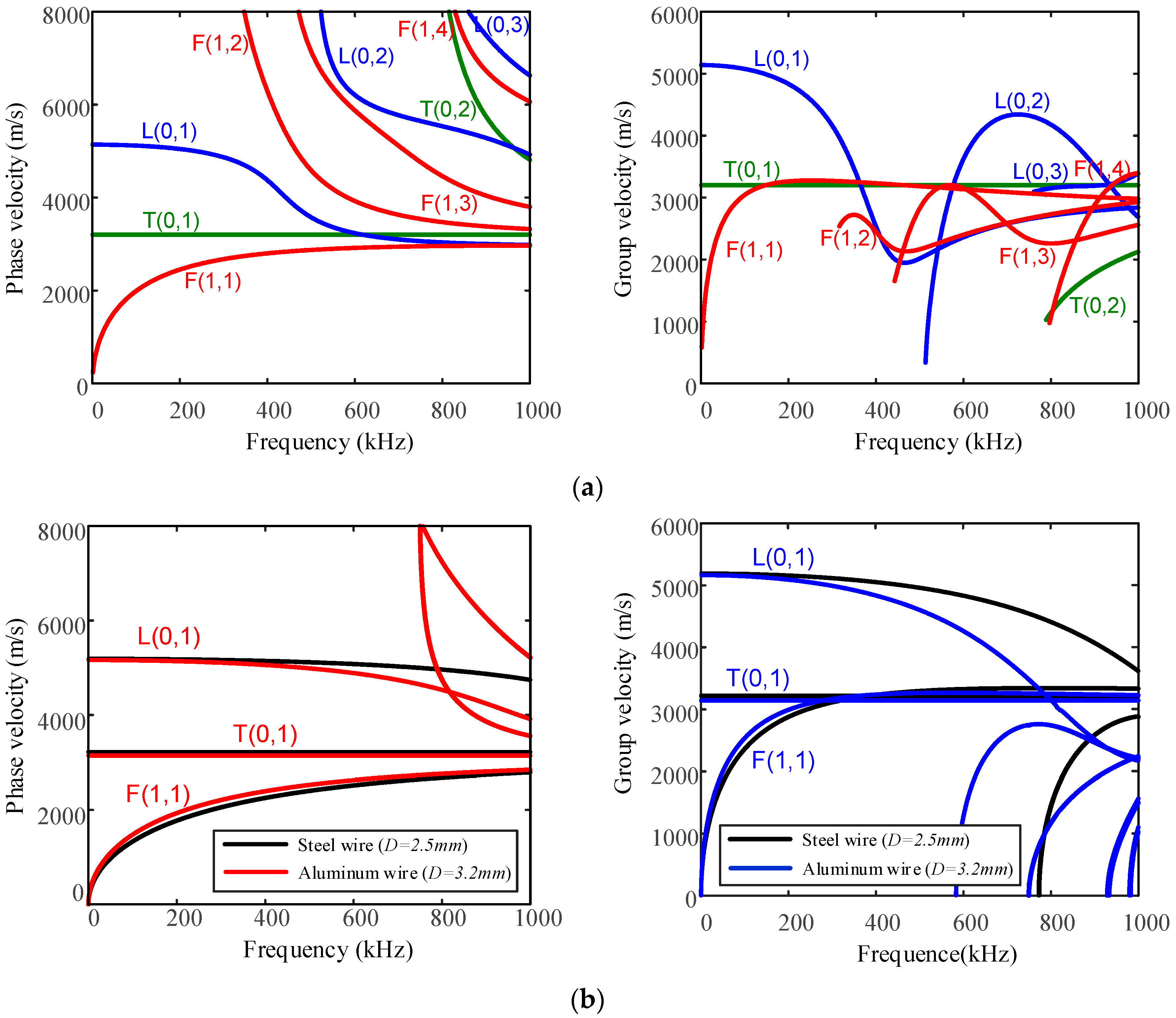
A single wire can be considered to be the same as an individual cylindrical rod, whose dispersion properties can be analytically obtained using the Pochhammer–Chree equations. UGWs tend to travel with different velocities in a structure depending on the center excitation frequency. There are two ways to define the propagation velocities of UGWs: group and phase velocity. Group velocity refers to the propagation velocity of the entire wave packet. Phase velocity is the propagation velocity at which the phase of any one frequency component of the wave travels. For a cylindrical rod, group and phase velocity dispersion curves of a 7-mm-diameter steel wire (commonly used in a bridge cable), and a steel and aluminum wire with a diameter of 2.5 mm and 3.2 mm, respectively (commonly used in ACSR cable), were acquired using an open source software package named PCDISP developed in the Matlab (MathWorks Inc., Natick, MA, USA) environment. PCDISP is described in more detail in references [28,29]. The material and geometric properties of wires used in the dispersion calculation models are summarized in Table 1. The results are shown in Figure 1.
Figure 1 shows UGW modes for three different types of wires with frequencies up to 1000 kHz. The phase and group velocities of the fundamental order flexural mode F(1,1) are slow and display severe dispersive properties in the low-frequency range (below 200 kHz). L(0,1) and T(0,1) seem to be the applicable modes for wire breakage inspection of steel and aluminum wires, though the velocity of the L(0,1) mode is faster than that of the T(0,1) mode at low frequencies, yet is slightly dispersive. Therefore, the L(0,1) mode seems ideal for wire breakage detection due to its velocity and relatively low dispersive behavior. Figure 2a–c show the vibration displacement distribution in a cross-section of a single 7-mm-diameter steel wire carrying these three types of fundamental modes: L(0,1), T(0,1), and F(1,1), at a frequency of 60 kHz. The arrows indicate the particle vibration displacements in the radial direction (in-plane). The color indicates the magnitude of the particle displacements in the z-axial direction (out-of-plane).
Both longitudinal and flexural guided waves create radial and axial vibration displacement. The coupling extent among the adjacent contact wires in the cable is determined by the radial vibration displacement at the wire surface (i.e., maximum radius). The larger the radial vibration displacement amplitude, the better the coupling. Therefore, the frequency of UGW wave modes with large radial vibration displacement at the wire surface become particularly critical during energy transfer. In Figure 2d,e, radial and axial vibration displacement distribution curves (wave structure) of the different radii of a 7-mm-diameter steel wire were calculated using Pochhammer–Chree equations for the L(0,1) and F(1,1) wave modes in the 20–180 kHz frequency range. As the wire radius increases, the radial displacements decrease but the axial displacements increase. This trend was significant with the increase in wave frequency below 200 kHz.
2.2. Contact Acoustic Nonlinearity of Coupled Double Rods
Higher harmonic ultrasonic waves are generated in a structure with imperfect interfaces, in which excited waves with a large amplitude are incident. This phenomenon is called the contact acoustic nonlinearity (CAN) effect [24]. This phenomenon is caused by the repeated reflection of incident waves between two surfaces. The same behavior occurs when a longitudinal UGW propagates to an imperfect interface formed by two surfaces of the contact structures. The compressional part of the wave can penetrate through the interface and propagate into another structure, but the tensile part cannot. Therefore, it is equivalent to a half-wave rectification of the transmitted wave, which is a nonlinear effect. This nonlinearity is embodied in the form of higher harmonics. In nondestructive inspection using a guided wave, when the characteristic length of the rough contact surfaces or a micro-crack is much smaller than the incident wavelength, a nonlinear phenomenon occurs.
In a pioneering work [30], the second harmonics generated by the nonlinear nature of the contact stiffness with the frequency of 2f was theoretically observed in both transmitted and reflected waves, where f is the frequency of incident waves. A pair of coupled waveguides were created with an active wire and a passive wire closely in contact with each other. An ultrasonic guided wave was excited on the left end of the active wire. The radial displacements of the active wire were partially coupled to the passive wire through contact stress in the contact interface. Additional waves were generated in the active and passive wires as a result of the local load provided by the contact stress, as shown in Figure 3.
2.3. Energy Model of Multi-Wire Waveguides
There are many limitations of modeling accurate UGW propagation of multi-wire structures taking into account the effect of mechanical contact, such as varying contact stress among the adjacent wires, wave mode conversion, and the CAN effect. In order to simplify the propagation model of an UGW in a multi-wire cable, a model that describes the transfer of the wave between an active and a passive wire from an energy perspective was used to analyze the propagation behavior of an UGW. A multi-wire system was composed of mechanically coupled wires. They were surrounded by a spring array along the wire axis [17,18]. Thus, the wave energy of the ith wire of a cable with n wires can be mathematically described by a second-order nonlinear differential equation:
where is the average energy transfer from all n wires to the ith wire, is the damping coefficient caused by the material, c is the mechanical coupling coefficient, and a binary constant indicates whether the wires i and j are in contact with each other, expressed as:
For a two-wire model, the equation can be solved using the ode-45 built-in algorithm in Matlab. The coupling coefficient, the material damping coefficient, and the initial conditions and were obtained using the method of least squares fitting to process the transient finite element (FE) simulation data shown in Section 3.2. The results are shown in Figure 4. With the propagation of the guided wave, the wave energy in the active wire was transferred to the passive wire. The wave energy in the two wires gradually decayed after reaching a balance, which was caused by material damping.
3. Transient Finite Element Simulations
The effective performance of the conventional transient FE technique for modeling UGW propagation in various structures has previously been demonstrated. Here, the transient solver ABAQUS® (Dassault System Inc., Paris, France) was employed to visually simulate UGW propagation in two different structures: an individual wire and two contact wires. The accuracy of the results is affected by the temporal and spatial resolution of signal acquisition in the FE simulation model. The time step for dynamic analysis (i.e., temporal sampling) and finite element size (i.e., spatial sampling) were determined by the maximum frequency (i.e., minimum wavelength) of the wave in the structure, which should meet the requirements of the Nyquist–Shannon sampling theorem [31]. An optimal spatial resolution is at least eight mesh nodes per wavelength [32,33]. The temporal sampling rate should be 10 times higher than the highest frequency component of the signal. The parameters of the FE simulation model are summarized as Table 2.
The dispersion of the dispersive guided wave propagating in a waveguide is relevant to the bandwidth of the excitation signal. The wider the bandwidth of the excitation signal, the greater the dispersion of the wave. In this paper, two types of excitation signals were used in the transient FE simulation to investigate the dispersion performance of the guided waves in the wire. First, the time-dependent triangular pulse signal was employed to excite a broadband signal with a frequency bandwidth exceeding 500 kHz, as shown in Figure 5a,b. Second, the Hann-windowed, five-cycle, 60 kHz sinusoidal tone burst was designed to excite the narrow bandwidth signal with a specific center frequency, as shown in Figure 5c,d.
The category of the UGW mode generation in a waveguide is related to the direction of the exciting loads. In order to achieve optimal excitation performance, the direction of vibration displacement of the loading was set to be consistent with the wave structure of the wave mode to be excited. According to the analysis of the wave structures of longitudinal and flexural guided waves in Section 2.1, the oblique imposed force with uniform components in the three directions was chosen to excite longitudinal and flexural mode waves. The perpendicular imposed force with a single component along the z-direction was chosen to excite pure longitudinal mode waves, as shown in Figure 6.
3.1. Single Wire
In order to analyze multimodal and dispersive guided wave signals, discrete wave signals in time and space were recorded at the receiving nodes of the FE model. Signals were mapped to dispersion data in the frequency and wavenumber domains applying the two-dimensional (2D) fast Fourier transform (FFT) method [34]. The essence of the 2D FFT is to perform two fast Fourier transforms on the signal, temporally and spatially. A guided wave signal is harmonical in time and space from the perspective of wave propagation. Therefore, the time and space domain signals can be mapped to angular frequency and wavenumber domain signals as:
where is the acceleration signal matrix recorded at the receiving nodes along the z axis of the wire, is the phase velocity, ω is the angular frequency, and is the wavenumber. In this case, the accelerations of 500 series with a spatial interval of 1 mm excited by a triangular pulse were used to extract the 2D FFT spectrum, as shown in Figure 7.
The theoretical phase velocity dispersion curves overlaid on the 2D FFT spectra in Figure 7 agreed with the transient simulation results for the longitudinal and flexural modes. As a result of the radial vibration displacement component and the z-axial vibration displacement component , excited by the oblique imposed forces along the x, y, and z directions, all longitudinal (i.e., L(0,1)) and flexural modes (i.e., F(1,1), F(1,2), and F(1,3)) below 500 kHz were generated in the single wire. On the other, the only the wave mode L(0,1) was excited by using the perpendicular triangular pulse along the z-direction.
In order to minimize the dispersion of guided waves during propagation in the structure, signals with a narrow bandwidth are commonly employed to excite waves for defect detection in structures. The tone burst consisting of several cycles of Hann-windowed sine waves is a typical narrow bandwidth signal, with the feature of: the larger the number of wave cycles, the narrower the bandwidth of the signal. Figure 8 shows the 2D FFT spectrum extracted from the nodal accelerations data recorded using the single wire FE model. The guided wave in the wire was excited with a Hann-windowed, five-cycle, 60 kHz sinusoidal tone burst perpendicular to the wire end face. The dispersion nephogram shows a section of the L(0,1) mode with bandwidth of about 40 kHz, which is the same as that of the excitation signal (see Figure 5b).
3.2. Two Contact Wires
When the two ends of the multi-wire cable are subjected to an axial tension, the wire-to-wire contact stress will appear between the adjacent wires. The magnitudes of the contact stresses are proportional to the axial tension. A simplified wire-to-wire contact model was employed to study the effect of contact stresses on UGW propagation in a multi-wire cable. The FE model was made up of two 7-mm-diameter parallel straight steel wires with the same length of 500 mm. One of the wires was active and the other was passive. This pair of wires was mechanically coupled in contact using uniform stresses. The contact stresses were provided by a static radial pressure equaling 70% of the ultimate tensile strength (UTS) of the wire. These contact stresses are called Hertzian contact stresses [35]. The contact condition between the two wires was modeled using a penalty friction formulation with the friction coefficient of 0.6.
The loading conditions in the FE simulations involved two stages: static load and dynamic load. The linear ramp signals were uniformly preloaded into two wires along the wire axes with opposite radial directions of the two wires. The static wire-to-wire contact and friction stresses were generated in this load step. In the second step, guided waves were excited by the dynamic load. An investigation of the wave propagation was conducted in two cases. In Case 1, the active wire was excited with an obliquely imposed triangular pulse force on one end face with equal components () along three directions. In Case 2, the active wire was excited with a Hann-windowed, five-cycle, 60 kHz sinusoidal tone burst perpendicular to the end face along the z-direction.
Acceleration data were recorded at the surface nodes of the FE elements of the two wires along the z-axis. The interval of the recorded points was set as 1 mm. The 2D FFT algorithm proposed in Section 3.1 was used again to compare the two cases to observe the change in the dispersion properties of UGWs in a pair of mechanically coupled wires. The 2D FFT transform spectra for the two cases are shown in Figure 9 and Figure 10.
In Figure 9, the dispersion nephograms in the 2D FFT spectra coincide with the theoretical phase velocity dispersion curves (see Figure 1a), which is consistent with the results obtained in the previously presented single wire case. The longitudinal mode (i.e., L(0,1)) and all flexural modes (i.e., F(1,1), F(1,2), and F(1,3)) below 500 kHz were generated in the active and passive wires. Guided waves in the passive wire are transferred by contact and friction stresses between two wires. The acoustic energy can be transferred into the adjacent wire when sufficient contact stresses occur on the interface of two wires. As a result of the leakage of energy, the guided wave modes and energy eventually trend to be the same, with the wave propagation in the two-wire system.
The CAN model described in Section 2.2. and the energy transfer model described in Section 2.3. provide two different perspectives and methods to analyze the dispersion properties and propagation behaviors of the guided wave in mechanically coupled structures. Acceleration data recorded on two wire surfaces with a narrow bandwidth excitation signal loaded on the active wire end face were transformed into 2D FFT spectra, as shown in Figure 10. Dispersion nephograms in the spectra of both the active and passive wire agree with the theoretical phase velocity dispersion curve of the single L(0,1) mode below 500 kHz. The directions of the excitation loads determine the generation of guided wave mode propagation in the structure. As a result of the contact stresses between the two wires, the CAN phenomenon of the active wire was observed. The additional frequency component of 120 kHz that doubles the excitation frequency of 60 kHz appeared in the spectrum. The frequency components in the passive wire covered a bandwidth range of 60–120 kHz. This may have occurred because the dispersion of guided waves in the passive wire transferred by contact stresses was more severe than that generated by direct excitation. From the perspective of energy transfer, the guided wave energy distribution in the active and passive wires fit the results of the energy-based model described in Section 2.3, as shown in Figure 4.
4. Experimental Analysis
4.1. Experimental Setup
Experimental verification of the proposed methods was performed on three types of samples. The first sample was a single 7-mm-diameter steel wire: the main component of the multi-wire bridge cable. The second sample was a pair of mechanically coupled 7-mm-diameter steel wires in contact. The third sample was an LGJ-400/35 ACSR cable (Tianhong Electric Power Fitting Co. Ltd., Zhejiang, China) comprised of two layers of seven steel wires and three layers of 48 aluminum wires, which were arranged helically in five layers (1–6–10–16–22). The diameter of the individual steel wire was 2.5 mm and the diameter of the aluminum wire was 3.2 mm. All these samples were the same length: 1.6 m.
A piezoelectric (PZT) UGW experimental inspection system was employed, as shown in Figure 11a. The pitch-catch method was used with a broadband excitation PZT transducer pasted to one end of the cable and the same reception transducer pasted to another cable end. The coupling radius of the transducer was 10 mm and the height of the transducer was 22 mm, as shown in Figure 11b. It had a broadband characteristic (frequency range of 30–150 kHz). The directivity of the transducer was perpendicular to the contact surface. Epoxy resin glue was used to paste the transducer to the wire surface.
For excitation, the transducer was driven by a personal computer (PC)-controlled preamplifier (RAM-5000, Ritec Inc., Warwick, RI, USA) with a Hann-windowed, five-cycle, sinusoidal tone burst. The excitation signal was applied to the transducer with an amplitude of 100 Vpp (peak-to-peak value). The detected voltage signals were filtered by a bandpass filter with a bandwidth of 150 kHz and a center frequency of 80 kHz, and amplified by about 41 dB. Then, the signal acquisition was conducted to the filtered signals with a sampling frequency of 2000 kHz. This routine was repeated 50 times with a pulse repetition frequency (PRF) of 20 Hz to remove random noise and achieve a higher signal-to-noise ratio (SNR). The signal series were averaged and processed using Matlab.
4.2. Single Wire
In these single wire experiments, four pitch-catch configuration cases were employed for guided wave dispersion verification. The center frequency of the exciting tone burst was 60 kHz. In Case 1, the exciting transducer was installed on the end face of the left end, and the receiving transducer was similarly installed on the end face of the right end. In Case 2, the exciting transducer was installed on the end face of the left end, but the receiving transducer was installed on the lateral face of the right end. In Case 3, the exciting transducer was installed on the lateral face of the left end, but the receiving transducer was installed on the end face of the right end. In Case 4, the exciting transducer was installed on the lateral face of the left end, and the receiving transducer was similarly installed on the lateral face of the right end.
The representation of a signal in the time and frequency domain can be expressed using a spectrogram. A spectrogram is a time-frequency plot obtained using time-frequency analysis, such as a continuous wavelet transform (CWT). It is a method used to measure experimental group velocity dispersion curves. Figure 12 shows the time-frequency spectrum of the received signals in the four experimental cases using the CWT method, over which the theoretical time-frequency group velocity dispersion curves are overlaid. The theoretical propagation time was calculated using:
where is the length of the wire and is the group velocities of all existent modes at each frequency between 0 kHz and 100 kHz. This process is equivalent to mapping the group velocity dispersion curves from the velocity-frequency domain to the time-frequency domain.
There were three guided wave modes in the 7-mm-diameter steel wire below 100 kHz, whose dispersion curves were described in Section 2.1. According to the wave structures plotted in Figure 2d,e, the radial and z-axial vibration displacements were the main components of the L(0,1) and F(1,1) modes at 60 kHz, respectively. Z-axial wave components were generated through horizontal excitation of the transducer. Radial wave components were generated through lateral excitation. Similarly, the horizontal and lateral reception methods of the transducer effortlessly received the z-axial and radial wave components.
Thus, the L(0,1) mode was highlighted in the measured group velocity dispersion nephograms shown in Figure 12a of Case 1. The same applied to the L(0,1) and F(1,1) modes in Cases 2 and 3 simultaneously, and F(1,1) in Case 4 individually. No torsional mode was highlighted in any of the four cases, since neither of the two excitation methods could generate a rotational displacement component.
4.3. Two Contact Wires
In order to analyze the CAN phenomena in a multi-wire cable, a wire-to-wire cable was first considered. Two identical 7-mm-diameter steel wires with a length of 1.6 m, used in previous experiments, were tied together tightly and compactly using nylon cable ties along the z-axial direction, as shown in Figure 11d. The wire that was excited to generate a UGW was labeled the active wire, and another one was labeled the passive wire. The installation of exciting and receiving transducers in Case 2 of Section 4.2. was employed to simultaneously receive L(0,1) and F(1,1) guided waves. The center excitation frequency of the tone burst was 60 kHz. The reception signals of the two wires were recorded and are plotted in Figure 13. The FFT spectra of the two signals were obtained. The theoretical group velocity dispersion curves calculated in Section 2.1. were used to determine the wave modes presented in the signals of two wires. There were two wave packets in the time domain signals of the active and passive wire: the direct waves of L(0,1) and F(1,1). The measured group velocities of two modes calculated from the time-of-flight (ToF) of the wave peak in two wave packets are consistent with the theoretical group velocity dispersion curves at 60 kHz.
The appearance of the frequency components of 120 kHz in the FFT spectrum of the active and passive wires, which was double the center frequency of the exciting signals, verifies the CAN effect of the two contact wires described in Section 2.2. and is consistent with the results of the transient FE simulation in Section 3.2.
4.4. Overhead Transmission Line
As described in Section 4.1, the third experimental sample LGJ-400/500 ACSR cable consisted of five layers (1–6–10–16–22) of wires composed of steel and aluminum. The innermost two layers were 7.5-mm-diameter seven-wire steel strands (1–6). Since the diameter of the single steel wire (D = 2.5 mm) was much smaller than that of the transducer (D = 10 mm), the entire steel strands were treated as one layer. The exciting transducer was installed on the end face of the strands’ end. The receiving transducers were installed on the lateral faces of four layers (7–10–16–22) of another cable end, as shown in Figure 14a.
Precise transient FE simulations that consider contact and friction stresses are computationally expensive. Applications of the FE method are limited to the multi-wire structures with short lengths and a smaller number of wires. For the sake of simplifying the description of UGW propagation behavior in multi-wire structures, such as bridge cables and ACSR cables, the energy-based model was used to investigate the experimental data. Guided wave signals recorded by transducers installed on each layer of the cable end (Z = 1.6 m) were processed by Matlab and are plotted in Figure 14b.
In Figure 14b, the signals from the top to bottom were received by the transducers installed on the first, second, third, and fourth layers of the cable (from the inside to the outside). The wave packet marked by a circle in each signal was the direct wave excited by the exciting transducer. As a result of the contact and friction stresses between the adjacent wires in the same and adjacent layer, wave energy was transferred to each wire of the cable with the guided wave propagation. Each wire in the inner layers of the cable was in contact with four adjacent wires: left wire, right wire, wire in the upper layer, and wire in the lower layer. Thus, the wave energy of each wire can be derived from Equation (1). The initial conditions in the equation were determined using a least squares fit with recorded signals. Since the active wire (first layer) was the steel strands in the center of the cable, the normalized wave energy of the wires in the same layer was equal (second, third, and fourth layers), as shown in Figure 14c. The measured wave energy can be obtained by integrating the received signal over the time domain:
where t1 and t2 correspond to the time required by the fastest and slowest modes at the frequency of 60 kHz propagating from to (i.e., and ), respectively, and is the radial vibration displacement at position z. The fastest and slowest mode at 60 kHz frequency in the 3.2-mm-diameter aluminum wire group velocity dispersion curves shown in Figure 1b were the L(0,1) mode and the F(1,1) mode, respectively.
5. Conclusions and Outlook
In this study, an initial theoretical analysis of UGWs in a two-contact-wire system and an ACSR cable was completed from various perspectives. A time-transient FE numerical simulation and experimental study were conducted to validate the dispersion and wave structure properties, the contact acoustic nonlinearity effect, and the energy transfer model of multilayer wires. The main findings are summarized as follows:
- (1)
- For the wave structures of the fundamental order longitudinal and flexural modes (i.e., L(0,1) and F(1,1)) in a 7-mm-diameter steel wire, the radial vibration displacements decreased but the axial vibration displacements increased with increasing radius. This trend became apparent with the increase in guided wave frequency below 200 kHz. The severity of dispersion and number of modes in a cylindrical structure were related to the bandwidth of excitation signals and the direction of excitation loads, respectively.
- (2)
- Guided waves with frequency f were excited to one of the two mechanically coupled wires. Received waves with frequency 2f were observed in both wires due to the CAN effect at the contact interface. Numerical and experimental verification were performed using a monokinetic Hann-windowed sinusoidal excitation. There are many different wave modes simultaneously propagating in a multi-wire structure with different velocities at different frequencies, which could be predicted by dispersion curves. However, it is ineffective for dispersion curves to analyze the frequency behaviors of the wave signals of a certain mode, which could be analyzed using the CAN effect.
- (3)
- A minimally computationally expensive energy transfer model was used to predict the wave energy distribution in the wires located in different layers of the multi-wire cable. The approach was applied to analyze a pair of mechanically coupled wires using transient FE simulation. The acceleration data of the two wires were fitted to the model. The same investigation was experimentally performed on a 1.6-m-long 55-wire ACSR cable, and the wave energy of each layer was found to be consistent with the numerical analysis. Uniform distribution of the wave energy in each layer of a multi-wire cable is a basic requirement of SHM using a guided wave. The uniformity of the UGW energy depends on the contact between adjacent layers, which can be predicted by the model, when using piezoelectric transducers installed on the outermost layer of the cable. The model also could be used to optimize the excitation power of transducers and determine the effective monitoring range of SHM. In industrial applications, the results of this study could be used to improve the detection rate of the defects of wires located in the inner layers of the cable with low signal amplitudes, which are caused by the nonuniform wave energy distribution in different layers of the cable.
For future research, we plan to study the UGW propagation in multi-wire cables using more precise contact and friction models to provide guidance for the guided wave inspection of cables, and the relationship between cable force and the CAN effect.
Author Contributions
P.Z. and Z.T. conceived and designed the models and methods presented; P.Z. developed the experimental software tools; F.L. and K.Y. helped in conception and experiments; Z.T. helped in the simulations; P.Z. performed the experiments and analyzed the data; and P.Z. wrote this paper.
Funding
This research was funded by the National Natural Science Foundation of China (Grant No. 61271084 and No. U1709216), the Science and Technique Plans of Zhejiang Province (Grant No. 2017C01042), the National Key Research and Development Program of China (Grant No. 2018YFC0809000), and the Project of Inner Mongolia Power Group (Grant No. 20184733). And The APC was funded by the National Natural Science Foundation of China.
Conflicts of Interest
The authors declare no conflict of interest.
References
- Shull, P.J. Nondestructive Evaluation: Theory, Techniques, and Applications; CRC Press: Boca Raton, FL, USA, 2016. [Google Scholar]
- Ye, X.W.; Dong, C.Z.; Liu, T. Force Monitoring of Steel Cables Using Vision-Based Sensing Technology: Methodology and Experimental Verification. Smart Struct. Syst. 2016, 18, 585–599. [Google Scholar] [CrossRef]
- Zhang, J.; Guo, Z.; Jiao, T.; Wang, M. Defect Detection of Aluminum Alloy Wheels in Radiography Images Using Adaptive Threshold and Morphological Reconstruction. Appl. Sci. 2018, 8, 2365. [Google Scholar] [CrossRef]
- Omidi, P.; Zafar, M.; Mozaffarzadeh, M.; Hariri, A.; Haung, X.; Orooji, M.; Nasiriavanaki, M. A Novel Dictionary-Based Image Reconstruction for Photoacoustic Computed Tomography. Appl. Sci. 2018, 8, 1570. [Google Scholar] [CrossRef]
- Qin, L.; Ren, H.; Dong, B.; Xing, F. Development of Technique Capable of Identifying Different Corrosion Stages in Reinforced Concrete. Appl. Acoust. 2015, 94, 53–56. [Google Scholar] [CrossRef]
- Shin, E.; Kang, B.; Chang, J. Real-Time Hifu Treatment Monitoring Using Pulse Inversion Ultrasonic Imaging. Appl. Sci. 2018, 8, 2219. [Google Scholar] [CrossRef]
- Zhang, J.; Tan, X.; Zheng, P. Non-Destructive Detection of Wire Rope Discontinuities From Residual Magnetic Field Images Using the Hilbert-Huang Transform and Compressed Sensing. Sensors 2017, 17, 608. [Google Scholar] [CrossRef] [PubMed]
- Mijarez, R.; Baltazar, A.; Rodríguez-Rodríguez, J.; Ramírez-Niño, J. Damage Detection in ACSR Cables Based on Ultrasonic Guided Waves. DYNA 2014, 81, 226–233. [Google Scholar] [CrossRef]
- Laguerre, L.; Treyssede, F. Non Destructive Evaluation of Seven-Wire Strands Using Ultrasonic Guided Waves. Eur. J. Environ. Civ. Eng. 2011, 15, 487–500. [Google Scholar] [CrossRef]
- Qian, J.; Chen, X.; Sun, L.; Yao, G.; Wang, X. Numerical and Experimental Identification of Seven Wire Strand Tensions Using Scale Energy Entropy Spectra of Ultrasonic Guided Waves. Shock Vib. 2018, 2018, 6905073. [Google Scholar] [CrossRef]
- Schaal, C.; Bischoff, S.; Gaul, L. Damage Detection in Multi-Wire Cables Using Guided Ultrasonic Waves. Struct. Health Monit. Int. J. 2016, 15, 279–288. [Google Scholar] [CrossRef]
- Zhang, P.; Tang, Z.; Duan, Y.; Yun, C.B.; Lv, F. Ultrasonic Guided Wave Approach Incorporating Safe for Detecting Wire Breakage in Bridge Cable. Smart Struct. Syst. 2018, 22, 481–493. [Google Scholar] [CrossRef]
- Rizzo, P. Ultrasonic Wave Propagation in Progressively Loaded Multi-Wire Strands. Exp. Mech. 2006, 46, 297–306. [Google Scholar] [CrossRef]
- Hernandez Crespo, B.; Courtney, C.; Engineer, B. Calculation of Guided Wave Dispersion Characteristics Using a Three-Transducer Measurement System. Appl. Sci. 2018, 8, 1253. [Google Scholar] [CrossRef]
- Raišutis, R.; Kažys, R.; Mažeika, L.; Žukauskas, E.; Samaitis, V.; Jankauskas, A. Ultrasonic Guided Wave-Based Testing Technique for Inspection of Multi-Wire Rope Structures. NDT E Int. 2014, 62, 40–49. [Google Scholar] [CrossRef]
- Raišutis, R.; Kažys, R.; Mažeika, L.; Samaitis, V.; Žukauskas, E. Propagation of Ultrasonic Guided Waves in Composite Multi-Wire Ropes. Materials 2016, 9, 451. [Google Scholar] [CrossRef] [PubMed]
- Schaal, C.; Bischoff, S.; Gaul, L. Energy-Based Models for Guided Ultrasonic Wave Propagation in Multi-Wire Cables. Int. J. Solids Struct. 2015, 64–65, 22–29. [Google Scholar] [CrossRef]
- Haag, T.; Beadle, B.M.; Sprenger, H.; Gaul, L. Wave-Based Defect Detection and Interwire Friction Modeling for Overhead Transmission Lines. Arch. Appl. Mech. 2009, 79, 517–528. [Google Scholar] [CrossRef]
- Hayashi, T.; Tamayama, C.; Murase, M. Wave Structure Analysis of Guided Waves in a Bar with an Arbitrary Cross-Section. Ultrasonics 2006, 44, 17–24. [Google Scholar] [CrossRef] [PubMed]
- Ibáñez, F.; Baltazar, A.; Mijarez, R. Detection of Damage in Multiwire Cables Based On Wavelet Entropy Evolution. Smart Mater. Struct. 2015, 24, 085036. [Google Scholar] [CrossRef]
- Treyssède, F. Elastic Waves in Helical Waveguides. Wave Motion 2008, 45, 457–470. [Google Scholar] [CrossRef]
- Li, C.; Han, Q.; Liu, Y.; Liu, X.; Wu, B. Investigation of Wave Propagation in Double Cylindrical Rods Considering the Effect of Prestress. J. Sound Vib. 2015, 353, 164–180. [Google Scholar] [CrossRef]
- Chillara, V.K.; Lissenden, C.J. Analysis of Second Harmonic Guided Waves in Pipes Using a Large Radius Asymptotic Approximation for Axis-Symmetric Longitudinal Modes. Ultrasonics 2013, 53, 862–869. [Google Scholar] [CrossRef] [PubMed]
- Jhang, K. Nonlinear Ultrasonic Techniques for Nondestructive Assessment of Micro Damage in Material: A Review. Int. J. Precis. Eng. Manuf. 2009, 10, 123–135. [Google Scholar] [CrossRef]
- Legg, M.; Yücel, M.K.; Kappatos, V.; Selcuk, C.; Gan, T. Increased Range of Ultrasonic Guided Wave Testing of Overhead Transmission Line Cables Using Dispersion Compensation. Ultrasonics 2015, 62, 35–45. [Google Scholar] [CrossRef] [PubMed]
- Gazis, D.C. Three-Dimensional Investigation of the Propagation of Waves in Hollow Circular Cylinders. I. Analytical Foundation. J. Acoust. Soc. Am. 1959, 31, 568–573. [Google Scholar] [CrossRef]
- Ditri, J.J.; Rose, J.L. Excitation of Guided Elastic Wave Modes in Hollow Cylinders by Applied Surface Tractions. J. Appl. Phys. 1992, 72, 2589–2597. [Google Scholar] [CrossRef]
- Seco, F.; Jiménez, A.R. Modelling the Generation and Propagation of Ultrasonic Signals in Cylindrical Waveguides. Ultrason. Waves 2012. [Google Scholar] [CrossRef]
- Seco, F.; Martín, J.M.; Jiménez, A.; Pons, J.L.; Calderón, L.; Ceres, R. Pcdisp: A Tool for the Simulation of Wave Propagation in Cylindrical Waveguides. In Proceedings of the 9th International Congress on Sound and Vibration, Orlando, FL, USA, 8–11 July 2002. [Google Scholar]
- Biwa, S.; Nakajima, S.; Ohno, N. On the Acoustic Nonlinearity of Solid-Solid Contact with Pressure-Dependent Interface Stiffness. J. Appl. Mech. 2004, 71, 508–515. [Google Scholar] [CrossRef]
- Abdul, J. The Shannon Sampling Theorem—Its Various Extensions and Applications: A tutorial review. Proc. IEEE 1977, 65, 1565–1596. [Google Scholar]
- Datta, D.; Kishore, N.N. Features of Ultrasonic Wave Propagation to Identify Defects in Composite Materials Modelled by Finite Element Method. NDT E Int. 1996, 29, 213–223. [Google Scholar] [CrossRef]
- Kirby, R. Modeling Sound Propagation in Acoustic Waveguides Using a Hybrid Numerical Method. J. Acoust. Soc. Am. 2008, 124, 1930–1940. [Google Scholar] [CrossRef]
- Alleyne, D.; Cawley, P. A Two-Dimensional Fourier Transform Method for the Measurement of Propagating Multimode Signals. J. Acoust. Soc. Am. 1991, 89, 1159–1168. [Google Scholar] [CrossRef]
- Johnson, K.L. Contact Mechanics; Cambridge University Press: Cambridge, UK, 1987. [Google Scholar]
Figure 1.
Phase and group velocity dispersion curves for (a) a single 7-mm-diameter steel wire and (b) a single steel and aluminum wire with a diameter of 2.5 mm and 3.2 mm, respectively.
Figure 1.
Phase and group velocity dispersion curves for (a) a single 7-mm-diameter steel wire and (b) a single steel and aluminum wire with a diameter of 2.5 mm and 3.2 mm, respectively.

Figure 2.
The vibration displacement distribution of (a) longitudinal, (b) torsional, and (c) flexural waves in a 7-mm-diameter steel wire. Wave structure of the (d) L(0,1) and (e) F(1,1) modes at different frequencies.
Figure 2.
The vibration displacement distribution of (a) longitudinal, (b) torsional, and (c) flexural waves in a 7-mm-diameter steel wire. Wave structure of the (d) L(0,1) and (e) F(1,1) modes at different frequencies.

Figure 3.
A schematic drawing of contact acoustic nonlinearity (CAN) at the rough contact interface of a pair of coupled cylindrical waveguides.
Figure 3.
A schematic drawing of contact acoustic nonlinearity (CAN) at the rough contact interface of a pair of coupled cylindrical waveguides.

Figure 4.
A model of the wave energy transfer between two adjacent wires. The results of the active wire are plotted by a red line, and the results of the passive wire are plotted by a blue line. The transient finite element (FE) simulation data of the two wires obtained in Section 3.2. are marked by asterisks.

Figure 5.
The excitation signal and fast Fourier transform (FFT) spectrum: the triangular pulse with a broadband of 500 kHz in the (a) time domain and (b) frequency domain; the Hann-windowed, five-cycle, 60 kHz sinusoidal tone burst in the (c) time domain signal and (d) frequency domain.
Figure 5.
The excitation signal and fast Fourier transform (FFT) spectrum: the triangular pulse with a broadband of 500 kHz in the (a) time domain and (b) frequency domain; the Hann-windowed, five-cycle, 60 kHz sinusoidal tone burst in the (c) time domain signal and (d) frequency domain.

Figure 6.
Guided waves in a single wire were excited using three loading methods: (a) an oblique triangular pulse with three equal components along the x, y, and z directions, (b) a perpendicular triangular pulse along the z-direction, and (c) a perpendicular sinusoidal tone burst along the z-direction.

Figure 7.
The phase velocity dispersion spectra obtained from nodal accelerations with different excitation methods: (a) an oblique triangular pulse signal with three equal components, and (b) a perpendicular triangular pulse signal with a z-axial component. The theoretical phase velocity dispersion curves obtained in Figure 1a are represented by the black dotted lines.

Figure 8.
The phase velocity dispersion spectrum from nodal accelerations with a Hann-windowed, five-cycle, 60 kHz sinusoidal tone burst along the z-direction. The theoretical phase velocity dispersion curve of the L(0,1) mode obtained in Figure 1a is represented by a black dotted line.
Figure 8.
The phase velocity dispersion spectrum from nodal accelerations with a Hann-windowed, five-cycle, 60 kHz sinusoidal tone burst along the z-direction. The theoretical phase velocity dispersion curve of the L(0,1) mode obtained in Figure 1a is represented by a black dotted line.

Figure 9.
The phase velocity dispersion spectra of two wires from nodal accelerations with an equal components triangular pulse force along the x, y, and z directions: (a) the active wire and (b) the passive wire. The theoretical phase velocity dispersion curves obtained in Figure 1a are represented by the black dotted lines.

Figure 10.
The phase velocity dispersion spectra of wires from nodal accelerations with a Hann-windowed, five-cycle, 60 kHz sinusoidal tone burst along the z-axial direction: (a) the active wire and (b) the passive wire. The theoretical dispersion curve of L(0,1) obtained in Figure 1a is represented by white dotted lines. (c) The FFT spectra of a representative received signal of the active wire and (d) part of the representative acceleration time-domain-received signals in the active wire.

Figure 11.
The experimental setup for guided wave excitation and reception in three types of samples. (a) The schematic of the experiment. Photos of (b) the piezoelectric (PZT) transducer, (c) the single wire experiment case, and (d) the two contact wires.
Figure 11.
The experimental setup for guided wave excitation and reception in three types of samples. (a) The schematic of the experiment. Photos of (b) the piezoelectric (PZT) transducer, (c) the single wire experiment case, and (d) the two contact wires.

Figure 12.
The time-frequency analysis spectrum using a continuous wavelet transform (CWT) for a single 7-mm-diameter steel wire at a 60-kHz frequency: (a) horizontal excitation and horizontal reception, (b) horizontal excitation but lateral reception, (c) lateral excitation but horizontal reception, and (d) lateral excitation and lateral reception. The theoretical group velocity dispersion curves obtained in Figure 1a are represented by the dotted line.

Figure 13.
The wave signals and FFT spectrum for the two contact wires with an exciting center frequency of 60 kHz: (a) the time domain signal of the active wire, (b) the FFT spectrum of the active wire, (c) the time domain signal of the passive wire, and (d) the FFT spectrum of the passive wire.
Figure 13.
The wave signals and FFT spectrum for the two contact wires with an exciting center frequency of 60 kHz: (a) the time domain signal of the active wire, (b) the FFT spectrum of the active wire, (c) the time domain signal of the passive wire, and (d) the FFT spectrum of the passive wire.

Figure 14.
Guided wave propagation experiments on the aluminum conductor steel-reinforced (ACSR) cable: (a) a photo of the exciting and receiving transducers installation, (b) the received time domain signals of each layer, and (c) the simulated and measured time average wave energy distribution in each layer.


Table 1.
The material and geometric properties of wires used in the dispersion models.
| Material | Diameter | Elastic Modulus | Density | Poisson Ratio |
|---|---|---|---|---|
| Steel | 7 mm | 209 GPa | 7800 kg/m3 | 0.3 |
| Steel | 2.5 mm | 209 GPa | 7800 kg/m3 | 0.3 |
| Aluminum | 3.2 mm | 72 GPa | 2700 kg/m3 | 0.35 |
Table 2.
The parameters of the transient FE simulation model.
| Diameter | Length | Density | Young Modulus | Poisson Ratio |
|---|---|---|---|---|
| 7 mm | 500 mm | 7800 kg/m3 | 209 GPa | 0.3 |
© 2019 by the authors. Licensee MDPI, Basel, Switzerland. This article is an open access article distributed under the terms and conditions of the Creative Commons Attribution (CC BY) license (http://creativecommons.org/licenses/by/4.0/).
Share and Cite
MDPI and ACS Style
Zhang, P.; Tang, Z.; Lv, F.; Yang, K. Numerical and Experimental Investigation of Guided Wave Propagation in a Multi-Wire Cable. Appl. Sci. 2019, 9, 1028. https://doi.org/10.3390/app9051028
AMA Style
Zhang P, Tang Z, Lv F, Yang K. Numerical and Experimental Investigation of Guided Wave Propagation in a Multi-Wire Cable. Applied Sciences. 2019; 9(5):1028. https://doi.org/10.3390/app9051028
Chicago/Turabian StyleZhang, Pengfei, Zhifeng Tang, Fuzai Lv, and Keji Yang. 2019. "Numerical and Experimental Investigation of Guided Wave Propagation in a Multi-Wire Cable" Applied Sciences 9, no. 5: 1028. https://doi.org/10.3390/app9051028
Note that from the first issue of 2016, this journal uses article numbers instead of page numbers. See further details here.