A Single Point-Based Multilevel Features Fusion and Pyramid Neighborhood Optimization Method for ALS Point Cloud Classification

Abstract

3D point cloud classification has wide applications in the field of scene understanding. Point cloud classification based on points can more accurately segment the boundary region between adjacent objects. In this paper, a point cloud classification algorithm based on a single point multilevel features fusion and pyramid neighborhood optimization are proposed for a Airborne Laser Scanning (ALS) point cloud. First, the proposed algorithm determines the neighborhood region of each point, after which the features of each single point are extracted. For the characteristics of the ALS point cloud, two new feature descriptors are proposed, i.e., a normal angle distribution histogram and latitude sampling histogram. Following this, multilevel features of a single point are constructed by multi-resolution of the point cloud and multi-neighborhood spaces. Next, the features are trained by the Support Vector Machine based on a Gaussian kernel function, and the points are classified by the trained model. Finally, a classification results optimization method based on a multi-scale pyramid neighborhood constructed by a multi-resolution point cloud is used. In the experiment, the algorithm is tested by a public dataset. The experimental results show that the proposed algorithm can effectively classify large-scale ALS point clouds. Compared with the existing algorithms, the proposed algorithm has a better classification performance.

1. Introduction

Airborne Laser Scanning (ALS) can capture large-scale point clouds of urban scenes. The point cloud classification of outdoor scenes can provide high-precision semantic maps for autonomous driving, improve the accuracy of vehicle positioning, and reconstruct a three-dimensional model of the city, which plays an important role in urban planning and dynamic management. In addition, it can improve the efficiency of resource utilization. Effectively labeling the correct class for all points in the scene is an important basis for the widespread adoption of point clouds [1,2,3,4]. However, a laser point cloud has a huge data number, high redundancy, and uneven scene distribution, which may lead to huge challenges in the point cloud classification. Therefore, it is of great significance to classify the three-dimensional point cloud in large outdoor scenes.

Currently, the number of point clouds with manual labeling in outdoor large scenes is not enough. However, machine learning can learn and classify point clouds in the case of less sample training data, and the speed is faster. At present, the point cloud classification methods can be mainly divided into two strategies: the single point-based classification and object-based classification methods.

The point-based point cloud classification is the classification of each individual point in a point cloud; this strategy uses points as the basic unit to extract features, train models, and predict class labels. There are three main steps: the neighborhood selection, feature extraction, and single point classification based on the features and classifiers.

(1) Neighborhood selection. In the neighborhood selection process, the commonly used point cloud neighborhood forms are: K nearest neighbors [5], radius neighborhoods [6], and column neighborhoods [7]. The parameter of neighborhood estimation is highly dependent on prior knowledge, and it is greatly affected by the change of the point cloud density [8,9]. For example, Hackel et al. constructed a multi-level scale pyramid, and a total of 144-dimensional features such as eigenvalues of the covariance matrix were extracted for each point in each pyramid. Subsequently, Random Forest was used for training and finally classified outdoor road scenes [10], and a better classification effect was obtained. Therefore, the selection based on multi-scale neighborhood is an important method for extracting single point effective features.

(2) Features extraction. The local feature of a point cloud is an abstract depiction of the environment around a given point. It is difficult to classify a point cloud by a single local feature. The common practice is to fuse multiple point cloud local features for classification. Normal and curvature are simple local features that clearly show some local information about the point cloud, such as the fact that the normal direction can represent the partial tangent plane of the point cloud, and the curvature can represent the smoothness of the point. For example, Fanxuan et al. [11] optimized the matching accuracy of point pairs in point clouds based on the curvature information, and the registration accuracy of point clouds was further improved. Geometric features are also common local features, also known as shape descriptors. For example, in the spin image [12], the main idea is to set up an image with the normal vector as the center; the image rotates around the axis. The number of 3D points encountered by each pixel in the point cloud is taken as its gray value. Finally, a two-dimensional array representing the local information of the three-dimensional space, that is, the rotated image feature, is obtained. The 3D Shape Context (3DSC) feature [13] is based on the specified point to construct a spherical region. In the support region, the grid is divided into three coordinate directions: the radial direction, direction angle and elevation angle. Following this, a feature histogram is constructed by entering the number of points in the grid. The 3DSC is simple in construction, strong in discrimination and insensitive to noise, but it is time-consuming. The Unique Shape Context (USC) descriptor [14] improves the 3DSC to avoid ambiguities in the classification. Point Feature Histograms (PFH) [15] are local features, which construct a feature histogram with the angles and distances of the normal vectors of any two points in the specified point neighborhood. The descriptor can accurately describe the local features of the points, but the computation is large and the real-time performance is poor. Fast Point Feature Histograms (FPFH) [16] are a simplification of PFH, which greatly reduce the time consumption while retaining most of the description performance of PFH. FPFH have an excellent performance, and are widely used in the field of point cloud classification, segmentation and registration [17]. Although these features can express the local features of the point cloud, they do not take into account the characteristics of the ALS point cloud, which has the characteristics of relative sparse, rich elevation information, as well as a horizontal and vertical distribution.

(3) Single point classification based on features and classifiers. Currently, machine learning is an important method for classification problems. The single-point classification based on machine learning takes the feature vector of the point as the input and the class label of the single point as the output. Common machine learning algorithms can accomplish this classification task, such as AdaBoost [18], Random Forest [19] and Support Vector Machine (SVM) [20]. This kind of method uses a classifier to learn the local features of each point, after which the parameters in the classifier are determined based on the training dataset. Finally, the test set is classified by the classifier. This classification strategy can more accurately segment the boundary regions between different adjacent objects, and this method has a better performance in detail. However, due to the extremely large number of points, the calculation amount is large. Thus, the model training is slow, and there are also some misclassifications of local regions. However, there are always some errors in the final classification results. Therefore, the initial classification results are required to further optimize according to the characteristics of the point cloud.

In order to solve the above-mentioned problems, an ALS point cloud classification algorithm based on a single point multi-feature fusion is proposed. This kind of algorithm is based on the point as the basic processing unit, and the classification process assigns labels to each point in the point cloud to realize a point cloud classification. The proposed method extracts the local features of each point by constructing a multi-scale neighborhood space, along with two new features: a normal angle distribution histogram (NAD) and latitude sampling histogram (LSH) are proposed. Following this, SVM is used for training and classification. However, since each point is classified, there is a problem regarding some edge points being misclassified. In this regard, the initial classification results are further optimized according to the neighborhood classification optimization of multi-scale pyramids. Experiments prove that the classification algorithm has a higher accuracy.

The main contributions of this paper are as follows:

(1) Two local features are proposed, that is, the NAD histogram and the LSH histogram. The differences of different objects in the normal distribution, and the difference of the neighborhood points around different objects in the horizontal and vertical directions of the three-dimensional space, can be fully utilized to more effectively represent the characteristics of different objects.

(2) A multilevel single-point features fusion method based on a multi-neighborhood space and multi-resolution is proposed. The multi-scale space is constructed by changing the resolution of the point cloud and the number of the neighborhood. The features of the multi-scale are extracted from each single point, and the features are fused. Following this, the SVM classifier is used to classify the features and the better classification results have also been achieved.

(3) A fast optimization method for classification results based on a multi-scale pyramid is proposed. By changing the resolution of the point cloud, a multi-scale pyramid is constructed, and the neighbor points are further re-selected. After this, the misclassifications are eliminated according to the initial classification results of the neighbors for a post-processing optimization.

2. Method

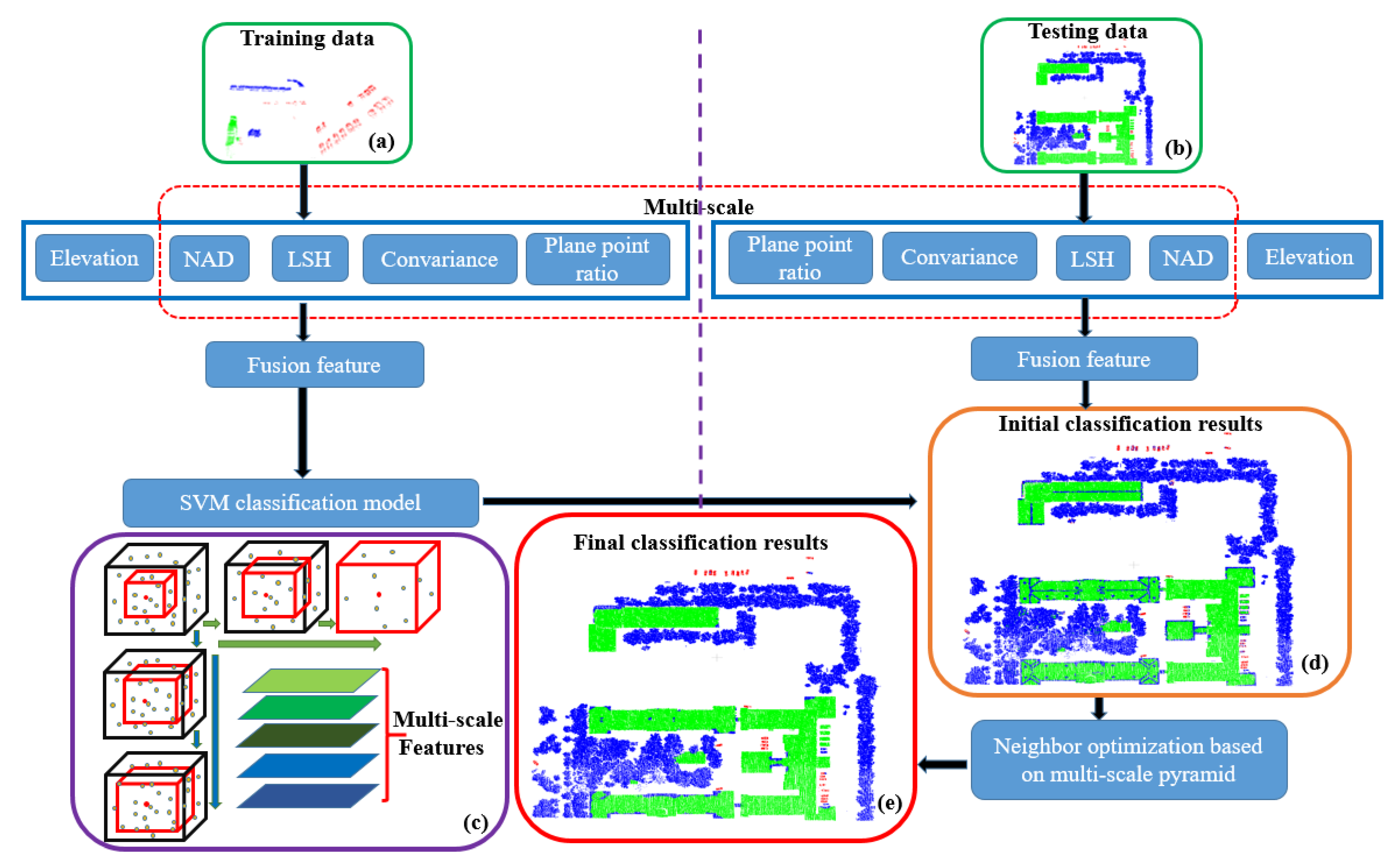
As shown in Figure 1, the algorithm flow is given as follows. In the training part, for the point cloud scene shown in Figure 1a, multiple features of each point are first extracted. Multi-scale and multiple features are fused to a fusion feature. The SVM classifier model is then trained using the fusion features of the training set. In the test part, for the point cloud scene shown in Figure 1b, the fusion feature is first obtained. As shown in Figure 1c, the test points are initially classified using the trained SVM classification model. Following this, the point clouds of different resolutions are obtained by down-sampling the point cloud, in order to construct a multi-scale point cloud pyramid. The corresponding classification labels of the different neighboring points in the different scales are searched. Finally, the label which has the most number in the neighbors is taken as the class label of the current point. The final point cloud classification result is obtained, as shown in Figure 1d.

2.1. Point Feature Extraction

In the classification task of the 3D point cloud data, the feature extraction of the point cloud plays a crucial role. It can seriously affect the final classification result. A well-behaved feature descriptor should reflect obvious differences between different types of points in the point cloud. At the same time, the descriptor should be robust and have a strong anti-interference ability. It is difficult for a single feature descriptor to have the above characteristics, so that a plurality of feature descriptor fusion methods are at present widely used. In the single point-based classification algorithm, this paper uses a variety of feature fusion methods to improve the accuracy of the classification algorithm. The specific features are as follows:

2.1.1. Feature Description

1.

Elevation feature

The height is a very intuitive feature in a 3D point cloud. Generally speaking, points with large height are buildings, trees or objects with larger elevation values in the real world. When the elevation value is small, the probability is greater if the point is a vehicle point. Thus, the elevation feature is set to:

$$F_z=[Z_i, \frac{1}{Z_i}]$$

(1)

where $Z_i$ is the distance of the i-th point from the estimated ground to the elevation value.

2.

Normal angle distribution histogram

In the large scale scene, the normal direction of different objects has obvious differences. For artificial objects, such as buildings and vehicles, since the surface is relatively regular, almost all points are in the same direction, pointing in the direction of the vertical plane. However, due to the scattered distribution of the whole point cloud, the normal direction of the point cloud has a large scattered nature, and the direction does not point to a fixed direction in a uniform way. Therefore, we calculate the histogram of each point and its own normal angle distribution value in the local neighborhood point set to express the relationship between the normal of the point and the normal of the points in the neighboring region. The angle between the two normal vectors in three-dimensional space should be between $[0,\pi ]$. But considering that the normal of the point on the plane can have opposite directions when the angle is larger than $\pi /2$, the corresponding angle is set to $\pi -\pi /2$. Following this, the angle of the normal vectors is defined as $[0,\pi /2]$. 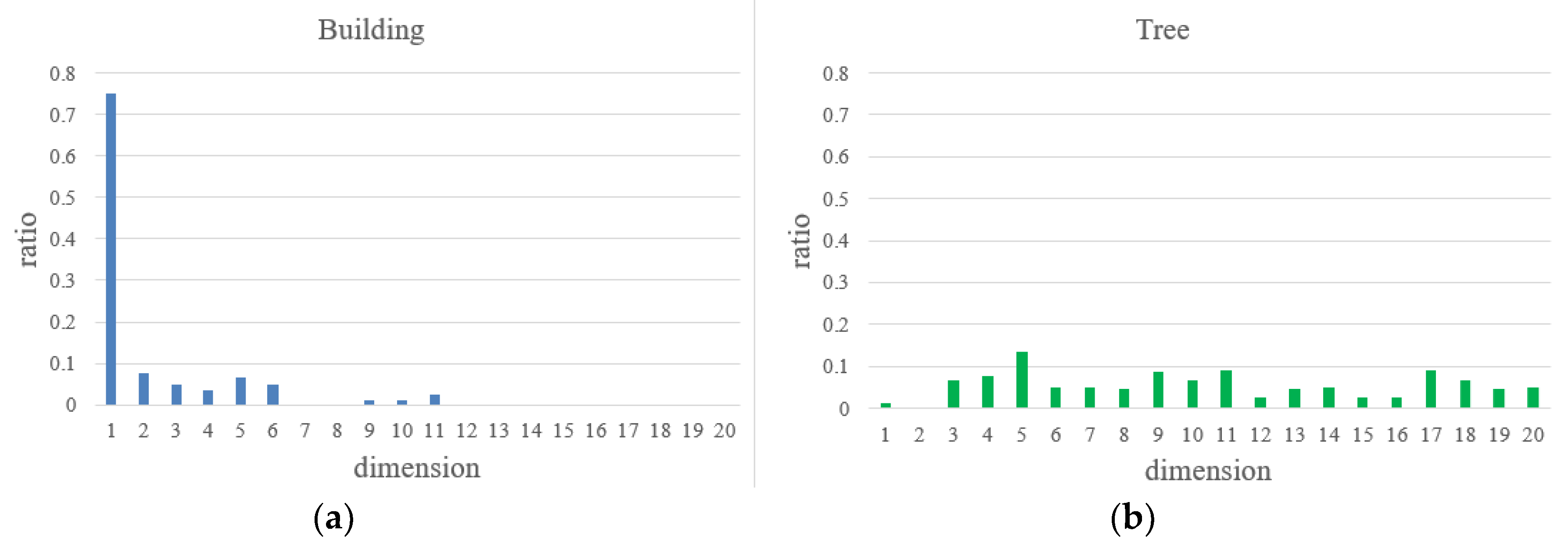Considering efficiency and resolving power, we divide this interval into equal $D_n$ parts, that is, construct a $D_n$ dimensional histogram. After this, the number of points falling within each cell is taken as the value of the interval in the histogram. Finally, the normalization process is performed to form a histogram of the normal angle distribution, called NAD. This feature can distinguish different classes of points based on the normal angular distributions. The specific calculation formulas are as follows:

$$∆=\frac{\pi /2-0}{D_n}$$

(2)

$${\theta }_j=\mathrm{a}\cos \left(v\cdot v_j\right)$$

(3)

$$h(x_i)=\frac{n(i\ast \Delta \le {\theta }_j\le (i+1)\ast \Delta )}{N}(i=1,\dots ,D_n)$$

(4)

$$F_{NAD}=\left[h\left(x_1\right),h\left(x_2\right),\dots ,h\left(x_{D_n}\right)\right]$$

(5)

where $v$ and $v_j$ represent the normal vectors of the current point and the j-th neighbor point, respectively. $\mathrm{a}\cos (\cdot )$ represents the inverse cosine function. N represents the number of neighbors for the current point. $n(i\ast \Delta \le {\theta }_j\le (i+1)\ast \Delta )$ denotes the number of points for the normal angle at the range $\left[i\ast \Delta ,(i+1)\ast \Delta \right]$. $F_{NAD}$ denotes the final normal angle eigenvalue vector of the normal angle distribution. The histogram of the normal angle distributions for the randomly selected building points and tree points are shown in Figure 2.

3.

Latitudinal sampling histogram

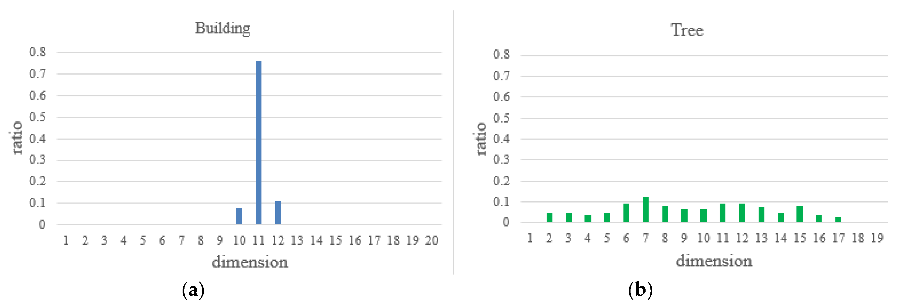
In the outdoor large scene environment, as for almost all points belonging to different objects, the surrounding neighborhood points have great differences in the latitudinal distribution in the three-dimensional space. For example, a building surface, which is parallel to the ground, has its neighborhood points mainly distributed near the “equator”. For the points belonging to the trees, the distribution of the neighborhood points is more random and extensive, hardly concentrated in a certain latitude interval. Therefore, the selected point is regarded as the center of the sphere, and the distribution histogram of the neighborhood points in the latitudinal direction is counted. Following this, the feature of the point can be expressed. The feature is called LSH. The LSH feature can be used to distinguish different classes of points according to the distribution of neighborhood points in the latitude direction. The LSH has the advantages of anti-occlusion, without interference from the local coordinate system, as well as high efficiency. In this paper, D_l spaces are equally divided along the latitude direction. Following this, the number of points falling into each cell is counted to form a feature vector of the D_l dimension. The specific calculation formulas are:

$$\Delta =\frac{\pi -0}{D_l}$$

(6)

$${\theta }_j=\mathrm{a}\cos \left(z\cdot \left(p_j-p\right)\right)$$

(7)

$$f\left(x_i\right)=\frac{n\left(i\ast \Delta \le {\theta }_j\le \left(i+1\right)\ast \Delta \right)}{N}(i=1,\dots ,D_l)$$

(8)

$$F_{LSH}=\left[f\left(x_1\right),f\left(x_2\right),\dots ,f\left(x_{D_l}\right)\right]$$

(9)

where $p$ and $p_j$ represent the three-dimensional coordinates of the current point and its j-th neighbor point, respectively. $z=\left(0,0,1\right)$ represents the unit vector of the positive direction of the $z$ axis. $n(i\ast \Delta \le {\theta }_j\le (i+1)\ast \Delta )$ represents the number of points in $\left[i\ast \Delta ,(i+1)\ast \Delta \right]$ of the neighborhood points along the latitudinal direction. $F_{LSH}$ represents the final feature vector of LSH. The LSHs of the randomly selected building points and tree points are compared, as shown in Figure 3.

4.

Convariance feature

First, a covariance matrix for the selected point neighborhood is constructed. After this, eigenvalues of the covariance matrix are calculated as: ${\lambda }_2\ge {\lambda }_1\ge {\lambda }_0\ge 0$, and the corresponding eigenvectors are calculated as: $v_2,v_1,v_0$. Here, the covariance feature (CF) is obtained according to the relationship among the eigenvalues, as follows:

Sum of eigenvalues:

$$F_{sum}={\lambda }_1+{\lambda }_2+{\lambda }_3$$

(10)

Full variance:

$$F_{omn}={\left({\lambda }_1\cdot {\lambda }_2\cdot {\lambda }_3\right)}^{\frac{1}{3}}$$

(11)

Anisotropy:

$$F_{ani}=\left({\lambda }_1-{\lambda }_3\right)/{\lambda }_1$$

(12)

Planarity:

$$F_{pla}=\left({\lambda }_2-{\lambda }_3\right)/{\lambda }_1$$

(13)

Linearity:

$$F_{lin}=\left({\lambda }_1-{\lambda }_2\right)/{\lambda }_1$$

(14)

Sphericity:

$$F_{sph}={\lambda }_3/{\lambda }_1$$

(15)

Following this, the final total covariance feature is: $F_{\mathrm{cov}}=\left[F_{sum},F_{omn},F_{ani},F_{pla},F_{lin},F_{sph}\right]$.

5.

Plane point ratio

In outdoor large scale scenes, the classes of objects are complex and the surface shapes are also different. However, a considerable part of the surface of artificial objects exhibits planar characteristics, such as buildings, vehicles, etc. Meanwhile vegetation does not have planar characteristics, so the plane point ratio of the local point cloud can be used as a local feature to classify point clouds. The covariance feature can also reflect the planar characteristics to a certain extent, but it is greatly interfered by noise. For this reason, the Random Sample Consensus (RANSAC) [21] is employed to fit the local neighborhood of the selected point. After this, the ratio of the plane points, called PPR (Plane Point Ratio), is calculated.

RANSAC is a method used to find the subset of data that is the best match for the model from the data set with random samples that are noisy but sufficient. The points matched with the model are called the inner points, and the points unmatched with the model are called the outer points. The plane is fitted using RANSAC as follows.

(1) Select three points randomly from all the neighborhood points and calculate the current model parameters. The model is as follows:

$$ax+by+cz+d=0$$

(16)

(2) Determine whether each point is an inlier, and then determine the inlier rate $\omega$ of the current model:

$$J_i=\{\begin{array}{c}1,\begin{array}{cc}& \end{array}{d}_i\le T_d\\ 0,\begin{array}{cc}& \end{array}{d}_i>T_d\end{array}$$

(17)

$$\omega =\frac{1}{N}{\displaystyle \sum _{i=1}^N{J}_i}$$

(18)

where d_i is the distance from the i-th point to the plane. T_d is a fixed threshold. J_i indicates whether it is an inlier or not. $N$ is the number of neighborhood points.

(3) If the current inlier rate is larger than the previous optimal inlier rate, the optimal inlier rate is updated.

(4) To find the optimal model, repeat steps (1) to (3) k times until the probability reaches P:

$$1-P\le {\left(1-{\omega }^3\right)}^k$$

(19)

The termination condition is:

$$k\ge \frac{\log \left(1-P\right)}{\log \left(1-{\omega }^3\right)}$$

(20)

When the RANSAC iteration is completed, the optimal inlier rate is the ratio of the plane points: $F_{plane}=\left[\omega \right]$.

2.1.2. Single Point Multi-Scale Multi-Feature Fusion

Since the features of the single point are dependent on the selected neighborhood space, different neighborhood spaces have different expression capabilities for different classes of point clouds. Additionally, the structure descriptions of point clouds with different resolutions also have certain differences. The local feature description of the single scale for a point is relatively single, and there are some noise points in the point cloud, which can make the simple feature of the single scale unable to accurately describe the feature of the single point. Therefore, a multilevel features fusion method based on the multi-neighborhood space and multi-resolution is proposed. As shown in Figure 1c, the proposed method constructs the multi-scale space by changing the resolution and the number of neighborhoods of the point cloud. Following this, multi-scale features for each single point in the point cloud are extracted. Because the elevation feature is not affected by the scale changing, we select NAD, LSH, CF and PPR features to construct the multi-scale features. We extract the features of a single point in each scale by choosing µ neighborhoods with different resolutions and $\mathsf{\upsilon }$ different neighborhood sizes under the original resolution. The multi-scale features of each point are expressed respectively as ${{\mathrm{F}}^{\prime }}_{\mathrm{NAD}}, {{\mathrm{F}}^{\prime }}_{\mathrm{LSH}}, {{\mathrm{F}}^{\prime }}_{\mathrm{cov}}, \mathrm{and}{{\mathrm{F}}^{\prime }}_{\mathrm{plane}}$. Considering the validity of the features and the efficiency of the calculation, this generally results in $2\le$ µ $+\mathsf{\upsilon }\le$ 5. In addition, the description of the single point feature only represents one characteristic of the point cloud. Therefore, it is necessary to fuse multiple features. After fusing the features, the multilevel features are expressed as follows:

$$F=\left[F_z,{F^{\prime }}_{NAD},{F^{\prime }}_{LSH},{F^{\prime }}_{cov},{F^{\prime }}_{plane}\right]$$

(21)

Because we aim at an ALS point cloud, the extracted elevation features are only two-dimensional and play an important role in the point cloud classification. In addition, when the point cloud features are extracted, the values of each feature have been normalized to [0, 1]. In order to reflect the role of the non-zero feature value, the feature should be normalized again according to Formula (22) when the extracted feature F is sparse. While the extracted feature F is not sparse, there is no need to normalize the feature. Therefore, the constructed feature is $X=\left[F_z^{*},F_{NAD}^{*},F_{LSH}^{*},F_{cov}^{*},F_{plane}^{*}\right].$

$$F_{i,j}^{*}=\frac{F_{i,j}-\min (F_j)}{\max (F_j)-\min (F_j)}$$

(22)

where $F_{i,j}^{*}$ is the value of the i-th row and the j-th column in the normalized feature matrix F*. $F_{i,j}$ is the value of the i-th row and the j-th column in the feature matrix F. $F_j$ is the vector of the j-th column (for all the points) in the feature matrix F.

2.2. Point Cloud Classification Based on SVM

SVM [22] is achieved by maximizing the classification interval in the feature space. For non-linear data, SVM maps them into a high-dimensional feature space by a kernel function, which make the data into linear separable data in a high-dimensional feature space. Following this, it realizes a classification by maximizing the interval. In view of the excellent generalization ability of SVM, we use SVM as a classifier for the single point classification in point cloud data. As we know, the correlation between the point cloud single point feature and neighbor points features, and the Gauss kernel function only has one parameter $\sigma$ and a low model complexity. Thus, in the absence of prior knowledge, the Gauss kernel function is often better than other kernels. Therefore, we choose the Gauss kernel function as the kernel function. Here, the Gauss kernel function of the SVM classifier is defined as follows:

The fused feature space is $\mathrm{X}$. The selected n d-dimensional feature samples $\left\{{\mathrm{x}}_1,{\mathrm{x}}_2,\dots ,{\mathrm{x}}_n\right\}$:

$$x_i=\left(x_{i1},x_{i2},\dots ,x_{id}\right){}^{\prime }ϵ{ℝ}^d$$

(23)

After the feature transformation, the feature space is Z. We map data in the X space to the Z space $z_i=\left(z_{i1},z_{i2},\dots ,z_{id}\right)ϵ{ℝ}^d$via the mapping function $\varphi (x)$. The function $K(x,z)$ satisfies the condition $K(x,z)=\varphi (x)\cdot \varphi (z)$, and the function $K(x,z)$ is a kernel function, while $\varphi (x)$ is a mapping function. The Gauss kernel function is as follows:

$$K\left(X,\mathit{z}\right)={{\displaystyle \sum }}_i^{n}K\left({\mathbf{x}}_i,\mathit{z}\right)={{\displaystyle \sum }}_i^n\exp (-\frac{{\Vert {\mathbf{x}}_i-\mathit{z}\Vert }^2}{2\sigma })$$

(24)

The corresponding decision function is:

$$f\left(\mathit{z},{\alpha }^{*},b^{*}\right)=sign({{\displaystyle \sum }}_i^n{y}_i{\alpha }^{*}\exp \left(-\frac{{\Vert {\mathbf{x}}_i-\mathit{z}\Vert }^2}{2\sigma }\right)+b^{*})$$

(25)

The SVM classifier is trained by the features of the training set, and the test set is classified by the trained classifier. The initial classification results for the point cloud in Figure 1b are shown in Figure 1d.

2.3. Neighborhood Optimization Based on Multi-Scale Pyramid

After the initial classification, the point clouds are basically classified correctly. Due to noise and other reasons, there are still some misclassifications in some details (such as edges). As shown in Figure 1d, most of the points in the scene have been correctly classified, and only a small part of them are misclassified. They mainly concentrate on edges and other places, and most of the points around the misclassified points are correctly classified. Therefore, it is necessary to further optimize the initial classification results to achieve a more accurate classification of the point clouds. Because local information is used as a feature to classify point clouds, the feature extraction relies heavily on a local region selection. In addition, the single point is taken as the basic unit of classification. Each point has its own characteristics, but because the two neighboring points are very close to each other and their neighborhoods are also very close, the extracted features will be very similar, which leads them to be more likely to be classified into the same class. Therefore, the neighbors of the misclassified points are also often misclassified. It is difficult to correct the misclassified points if only the points in the smaller local regions are used for the optimization. Therefore, we propose a classification results optimization method based on the multi-scale pyramid. The specific method is as follows:

First, voxel filters with different radius scales are used to down-sample the point cloud after an initial classification, as shown in Formula (24). Each minimum voxel scale is twice as large as the last down-sampling, and sparse point clouds are gradually obtained. Following this, the q-level pyramid is constructed, and the initial classes of all the points in each level are retained. According to the characteristics of the point cloud down-sampling reflecting the structure information of the shape, the scale pyramid is constructed on three scales of q = 3 in this paper.

Following this, the corresponding k-d tree is constructed from the point cloud in each layer of the pyramid. For each point in the original point cloud, a k-d tree is used to search for the radius of the nearest neighbors in the point cloud after the down-sampling. The class labels of the m point clouds searched within the radius of the l-th level are $L^l=\left\{L_1^l,\dots ,L_m^l\right\},L_i^l\in \left\{1,\dots ,c\right\}$, i = 1,…, m, l = 1,.., q; the radius parameters are different when each layer of the point cloud chooses its nearest neighbor. The method of calculation is as follows:

$$r=k\cdot Presolution$$

(26)

In the formula, r represents the scale radius parameter. $Presolution$ is the resolution used by the current down-sampling point cloud. k is a fixed ratio threshold.

Finally, the initial labels of all the nearest neighbors in the q levels are counted. The discriminant function $1\left\{L_i^l=C\right\}$ represents the fact that when$L_i^l$ belongs to class C, its value is 1; otherwise, its value is 0. This is used to count the number of the initial labels belonging to each class. As shown in Formula (27), the mode label $C^{*}$ is selected as the new class label for the current point.

$$C^{*}=\begin{array}{c}\arg \max {{\displaystyle \sum }}_{l=1}^q{{\displaystyle \sum }}_i^{m}1\left\{L_i^l=C\right\} \\ C=L_i^l\in \left\{1,\dots ,c\right\} \end{array}$$

(27)

Not only do the optimized point cloud classification results avoid a situation where the nearest neighbor is also misclassified, but they also solve the problem of too many far points in a large scale, thus achieving better results. The optimized point cloud classification results are shown in Figure 1e.

3. Experimental Results and Analysis

In order to verify the performance of the point cloud classification algorithm based on single point multilevel features, we use two urban scenes’ ALS data for a qualitative and quantitative comparison and analysis. This section begins by briefly introducing the experimental data, before the classification performance of the proposed method is compared with the other methods on the datasets.

3.1. Experimental Dataset

In this paper, we use two sets of dataset published in Ref [23]. The data was collected in Tianjin, China. The density of the test region point cloud is about $20~30/{\mathrm{m}}^2$. The data set contains both large objects (buildings and trees) and small objects (cars). It contains different roof shapes, buildings of different heights, and dense and overlapping cars and trees.

Table 1. The experimental dataset.

Scene	Training Points			Test Points
	Tree	Building	Car	Tree	Building	Car
Scene 1	68,802	37,128	5380	213,990	200,549	7816
Scene 2	39,743	64,952	4584	73,207	156,186	7409

lists the number of each class point for the two scenes. Figure 4a,b shows the training data of scene 1 and scene 2, respectively.

All the programs are run on a computer with an Intel Core i7-7700K CPU, 4.20 GHz with 24-GB RAM. The algorithm is implemented on the C++ platform based on PCL 1.8.0. Each set of data training and testing takes about 6.5 min. However, the feature extraction and optimization process can be implemented in parallel. Therefore, the efficiency of the proposed method can be further improved, and the speed of the point cloud processing will be greatly improved.

3.2. Experimental Comparison and Analysis

In order to verify the performance of the proposed algorithm, we compare it with the other seven methods shown in

Table 2. Main features of the proposed method and other comparison methods. SVM: Support Vector Machine; LDA: Latent Dirichlet Allocation; DD-SCLDA: Discriminative Dictionary based Sparse Coding and LDA.

Method	Scale	Feature Expression	Post-Processing Optimization	Classifier
Our method	Multi-scale	Fz+FNAD+FLSH+Fcov+Fplane	Multi-scale pyramid	SVM
Method 1	Multi-scale	Fz+Fcov+Fplane	Multi-scale pyramid	SVM
Method 2	Single scale	Fz+FNAD+FLSH+Fcov+Fplane	None	SVM
Method 3	Single scale	Fz+FNAD+FLSH+Fcov+Fplane	Multi-scale pyramid	SVM
Method 4	Multi-scale	Geometry, strength, and statistical features	Regional growth	JointBoost
Method 5	Multi-scale	Spin Image feature and Fcov	None	AdaBoost
Method 6	Multi-scale	LDA Model of the Spin Image feature and Fcov based on Multi-Level Point Sets	None	AdaBoost
Method 7	Multi-scale	DD-SCLDA Model of the Spin Image feature and Fcov based on Multi-Level Point Sets	None	AdaBoost

. Method 1 is the proposed method, which uses the features without NAD and LSH. Method 2 uses the F_z+F_NAD+F_LSH+F_cov+F_plane feature fusion in single-scale without a post-processing optimization. Method 3 uses the single-scale feature and multi-scale pyramid optimization. Method 4 is the algorithm proposed in [24]. In this method, each feature uses geometry, strength, and statistics information. Following this, the JointBoost method is used to select features and classify points. Method 5 is the classification method based on the multi-scale Spin Image feature and F_cov feature fusion used in Ref [23]. Method 6 [25] constructs a multilevel point set using a linear transformation, and it uses Spin Image and F_cov features. Following this, K-means is used to construct an LDA (Latent Dirichlet Allocation) model of a multilevel point set dictionary. Method 7 [23,26,27] constructs a multilevel point set using an exponential transformation. The Spin Image and F_cov features are used for dictionary learning, constructing an LDA model of point sets.

Accuracy, precision, and recall are often used to evaluate the effect of a point cloud classification [27]. The precision rate is the proportion of true positive samples in a positively predicted sample. The recall rate is the proportion of positive samples that are predicted to be successful in the actual positive samples. The accuracy rate is the ratio of all the correctly predicted samples in relation to the overall samples. In order to consider both P_a (precision rate) and R (recall rate), F₁-score values (such as Equation (28)) are generally used to represent the classification quality of the scene. In order to better evaluate the effects of each algorithm, we use the above metrics to evaluate the classification performance.

$$F_1-score=\frac{2\left(R\times P_a\right)}{R+P_a}$$

(28)

The classification results of our method and of other comparison methods on scene 1 and scene 2 are shown in

Table 3. Classification results of precision/recall, accuracy and F₁-score.

Scene 1	Tree (%)	Building (%)	Car (%)	Accuracy (%)	F1-Score (%)
Our method	99.2/90.6	91.1/99.3	92.9/48.2	94.6	94.5/94.9/59.5
Method 1	99.2/84.9	86.8/99.3	99.9/42.7	91.9	91.5/92.7/59.8
Method 2	93.2/78.7	82.1/94.6	63.3/30.4	86.4	85.3/87.9/41.1
Method 3	96.9/81.7	84.1/97.7	98.8/23.2	89.3	88.7/90.4/37.6
Method 4	89.7/98.1	97.9/89.1	65.2/46.6	92.9	93.7/93.3/54.4
Method 5	85.7/92.9	92.0/83.8	56.9/54.7	87.9	89.2/87.7/55.8
Method 6	94.8/93.8	93.5/92.3	41.2/66.7	92.6	94.3/92.9/50.9
Method 7	93.1/96.0	95.2/92.6	73.3/62.2	93.7	94.5/93.9/67.3
Scene 2	Tree (%)	Building (%)	Car (%)	Accuracy (%)	F1-score (%)
Our method	92.4/94.3	98.5/97.9	73.0/68.4	95.8	93.4/98.2/70.6
Method 1	83.2/92.9	98.5/92.8	62.6/65.7	92.0	87.8/95.6/64.1
Method 2	77.3/94.3	98.3/88.9	71.7/60.0	89.6	85.0/93.4/65.3
Method 3	91.3/92.6	96.6/96.6	63.2/55.5	93.4	91.9/96.6/59.1
Method 4	86.8/91.2	96.8/95.5	44.1/34.8	92.2	88.9/96.1/38.9
Method 5	73.9/91.2	93.6/88.2	29.5/25.4	87.2	81.6/90.8/27.3
Method 6	90.3/93.9	97.6/96.5	49.4/42.0	94.1	92.1/97.0/45.4
Method 7	94.7/94.5	98.1/97.7	53.9/60.5	95.5	94.6/97.9/57.0

. Table 3 lists the precision, recall, accuracy and F₁-score statistics for the eight methods in the two scenes. It can be seen from Table 3 that the comparison between the proposed method and Method 1 shows that the accuracy of the proposed method has significantly improved. It also shows that the proposed NAD and LSH features have certain effects. By comparing Method 2 and Method 3, the proposed multi-scale pyramid optimization algorithm can effectively improve the classification accuracy. Comparing the proposed method with Method 3, the proposed multi-scale strategy has a significant effect on the improvement of the classification results.

In addition, the proposed method is compared with the methods given in other references. Method 4 and Method 5 classify the point cloud based on the single-point. Method 6 and Method 7 classify the point cloud based on the point set (object). It can be seen from the comparison of Table 3 that the proposed method has a high accuracy rate as a whole, and that it also maintains a high recall rate.

For scene 1, the accuracy of the proposed method is the highest, and the value of the precision/recall is relatively high (the classification result of the proposed method is shown in Figure 1e). From the classification results evaluation of the three kinds of objects by the F₁-score, one can see that the classification effect on cars for the proposed method is not as good as for Method 7. Meanwhile, the tree and building classes can basically be classified correctly.

For scene 2, the precision/recall of trees of the proposed method are lower than for Method 7. Meanwhile, the precision/recall of buildings and cars are the maximum compared with other methods. According to the classification result of the F₁-score value, the proposed method has a better effect than the other methods, except that the tree classification performance is worse than for Method 7. Considering the accuracy, precision/recall rate and the F₁-score evaluation comprehensively, the proposed method has a better classification performance than the other methods, and the proposed method has the highest overall accuracy for both scenes. This proves that the proposed point cloud classification method based on point multilevel features is effective, and that it can accurately classify the ALS point cloud data in large scale scenes.

In order to more intuitively compare the classification performance of each method, Figure 5 shows the performance of the eight classification methods in scene 2. Figure 5 shows that the proposed method can classify most points correctly. Compared with other comparison methods, the classification accuracy of the proposed method is higher. From the comparison between Figure 5c–e and Figure 5b, the classification effect of the proposed method is obviously better than that of the other three algorithms, especially in the buildings and trees. It can be seen from the comparison between Figure 5f,g and Figure 5b that Method 4 and Method 5 have more misclassifications for cars and buildings, and that the performance of the proposed method is significantly better than that of the other two methods. In comparing Figure 5h,i with Figure 5b, one can see that Method 6 and Method 7 have a similar classification performance to that of the proposed method. However, a certain number of architectural edge points are classified incorrectly, and the top part of the trees is also classified incorrectly. One can see from the comparison between Figure 5f–i and Figure 5b that the compared methods have some misclassifications for the edge points and for two objects that are overlapping regions. However, the proposed method has fewer misclassifications in those regions than for the other methods. This proves that the proposed feature descriptors and post-optimization strategies can improve the classification results.

3.3. Sensitivity of the Parameters

In this part, we focus on the $D_m$ in NAD, $D_l$ in LSH and the number of neighborhood scales (µ $+\mathsf{\upsilon }$). Here, we select the parameters shown in

Table 4. Parameters comparison based on mF₁ and Accuracy.

	Dm	Dl	$\mathsf{\mu }+\mathsf{\upsilon }$	Tree (%)	Building (%)	Car (%)	Accuracy (%)	mF1 (%)
1	10	10	3	94.0	94.4	60.7	93.9	82.9
2	15	10	3	94.0	94.5	60.7	94.0	83.1
3	20	10	3	93.9	94.5	60.3	94.0	82.9
4	15	15	3	94.7	95.0	63.5	94.6	84.4
5	15	20	3	94.3	94.7	60.2	94.3	83.1
6	15	15	4	94.7	95.0	62.6	94.6	84.1
7	15	15	5	94.7	95.0	62.6	94.6	83.8
8	20	20	2	93.5	94.1	54.5	93.5	80.7
9	20	20	3	94.5	94.9	59.5	94.4	83.0
10	20	20	5	94.5	94.9	59.0	94.4	82.8

; the data of scene 1 is used to compare the influence of different parameters on the proposed method. In order to evaluate the classification effect of the three kinds of objects as a whole, we average the F₁–score values of the three object classification results to obtain the mean value mF₁, which is used as the overall classification effect evaluation metric. As shown in Table 4, considering the results of mF₁ and the accuracy in combination, in comparing the parameters of the first three rows one can see that when $D_m$ is 15, the classification effect is better; however, the value of $D_m$ is not sensitive to the classification effect. According to the results of rows 2, 4 and 5, the classification effect of $D_l$ is obviously improved at 15. However, when the value of $D_l$ is too large, the classification effect is reduced. Therefore, the value of $D_l$ is relatively sensitive to the classification result. According to the results of rows 4, 6, 7 and 8–10, the classification effect is improved when the value of the scale µ $+\mathsf{\upsilon }$ is increased. However, when the scale exceeds 4, the classification effect will be reduced to some extent. Therefore, the value of the scale is sensitive to the results of the classification and needs to be within a reasonable range. One can see from Table 4 that the tree and building classes are relatively less affected by the changes of the $D_m$ and $D_l$, and that the results are susceptible to the size of the scale. The increasing values of $D_m$ and $D_l$ would likely cause a change in the car classification effect. Considering the overall effect of the classification and the factors of accuracy and feature dimension, we select $D_m$ = 15, $D_l$ = 15 and (µ $+\mathsf{\upsilon }$) = 3 as the optimal parameter values.

4. Conclusions

The classification of the ALS point cloud is an important technology for urban planning, digital city and intelligent transportation. We propose a multilevel features fusion and pyramid neighborhood optimization ALS point cloud classification method based on a single point. The proposed method presents two local features, i.e., the NAD and LSH. They are fused with the covariance and elevation features. Following this, the multilevel features are constructed by changing the point cloud resolution and the neighborhood size. The fused features are used to train a classification model based on the Gaussian kernel function SVM for an initial classification. Finally, the point cloud classification is optimized based on the initial classification result using a multi-scale pyramid. The optimized classification results have a higher accuracy. The experimental results prove the effectiveness of the proposed method via the experiments on the two sets of public ALS datasets.