Article

Deep Fusion Feature Based Object Detection Method for High Resolution Optical Remote Sensing Images

1
Harbin Institute of Technology, Shenzhen 518055, China
2
School of Computer Engineering, Shenzhen Polytechnic, Shenzhen 518055, China
3
Department of Computer Science, University of Hong Kong, Pokfulam Road, Hong Kong, China
*
Author to whom correspondence should be addressed.
Appl. Sci. 2019, 9(6), 1130; https://doi.org/10.3390/app9061130
Submission received: 31 January 2019 / Revised: 22 February 2019 / Accepted: 27 February 2019 / Published: 18 March 2019

Abstract

:
With the rapid growth of high-resolution remote sensing image-based applications, one of the fundamental problems in managing the increasing number of remote sensing images is automatic object detection. In this paper, we present a fusion feature-based deep learning approach to detect objects in high-resolution remote sensing images. It employs fine-tuning from ImageNet as a pre-training model to address the challenge of it lacking a large amount of training datasets in remote sensing. Besides, we improve the binarized normed gradients algorithm by multiple weak feature scoring models for candidate window selection and design a deep fusion feature extraction method with the context feature and object feature. Experiments are performed on different sizes of high-resolution optical remote sensing images. The results show that our model is better than regular models, and the average detection accuracy is 8.86% higher than objNet.

1. Introduction

Object detection for remote sensing images is an important research field. With the development of remote sensing technology, information carried by remote sensing images is more abundant than before. The applications of object detection in remote sensing images are more and more popular, such as city planning and environmental exploration.
However, object detection for remote sensing images is a more difficult job since remote sensing images are quite different from regular images. Objects in regular images have some properties: many objects rarely appear in one image; the main objects are regularly located in the image center, occupying the main parts and significantly different from the background.
However, one high-resolution optical remote sensing image contains more objects with more shapes and texture information than a regular image, and the objects may be scattered in the whole image. Besides, the object to be detected is relatively small and close to the background. If we zoom out from a remote sensing image to a small size for a global view, we would lose many details, and the objects may almost be invisible. Therefore, object detection for remote sensing images is harder work than for regular images to some extent.
At present, object detection methods in remote sensing images are mainly based on traditional image processing technology with machine learning, which requires rich experience and complete prior knowledge. Furthermore, most of them are only effective in a specific environment, so they have poor scalability. With the advent of deep learning technology, we introduce deep learning into the field of object detection for remote sensing images. Nevertheless, deep learning is still in its infancy for remote sensing images. One of its biggest problems is the decency on labeled datasets.
However, with the fast improvement of deep learning-based object detection on regular images, many labeled regular image datasets have appeared in recent years. Therefore, in this paper, we present a novel transfer deep learning approach to detect objects in high-resolution remote sensing images. It employs transfer learning to supply the gap that deep learning on remote sensing images lacks labeled training datasets. Besides, we improved the candidate window selection process and designed a deep feature extraction method with context scene feature fusion and detection. Finally, the proposed approach is validated on different scales of high-resolution optical remote sensing images.
This paper is organized as follows: Section 2 introduces the related works. Section 3 describes the framework of our algorithm. Our size-scalable region proposal algorithm is given in Section 4. Our deep feature extraction method with context scene feature fusion and detection is proposed in Section 5. Section 6 concludes the paper.

2. Related Works

The development of object detection in high-resolution remote sensing images has been in three stages: template matching-based, knowledge testing-based, and machine learning-based.
Weber et al. [1] performed template matching by extending the hit-or-miss transformation in a multivariate fashion to detect storage tanks and the shoreline. Sirmacek et al. [2] demonstrated the detection of urban buildings by using the SIFT feature to represent a two-building template. Knowledge testing-based object detection transforms detection into the hypothesis testing problem by establishing a set of knowledge and rules. Yokoya et al. [3] used buildings and shadows to detect buildings of arbitrary shape automatically. Machine learning-based methods have been the main direction of object detection in the remote sensing field. For example, Tao et al. [4] described the airplane objects by a set of key point SIFT feature and a graph model to detect them. Sun et al. [5] constructed a bag-of-words model by clustering SIFT feature points to represent targets and classified them by SVM. Gan et al. [6] performed ship detection on remote sensing images by extracting the HOG feature of the sliding window and extracted the continuous window feature by rotating the sliding window to achieve certain rotation invariance. Mostafa et al. [7] clustered the urban railroad point clouds into three classes of rail track, contact cable, and catenary cable by a template matching approach. Aytekin et al. [8] automatically selected a representative subset of texture features by the AdaBoost algorithm and used them to identify airport runways and then detect the airport. Felzenszwalb et al. [9] obtained good results in general object detection by combining the pyramid HOG feature with the partial deformation model and training an SVM with hidden variables. Some scholars have applied weak-supervised object detection algorithms to remote sensing images [10].
However, these methods mostly relied on a variety of well-designed prior knowledge or shallow features, etc. [11,12]. That is, they require a wealth of experience and a tedious trial and error process, and they have limitations.
In the field of object detection on regular images, Krizhevsky et al. [13] proposed an image classification algorithm based on deep learning, which automatically extracts the higher level features of the images by a convolutional neural network (CNN), which made the image classification task more concise and the classification accuracy significantly better.
Thanks to the development of deep learning and the development of region proposal algorithms, the object detection field has also made great breakthroughs. One of the main challenges of object detection in remote sensing images is how to reduce the computational complexity. In view of the large scale of remotely-sensed images, there will be a large number of candidates if the conventional multi-scale scanning window exhaustive strategy is used to obtain the region of interest, which makes the subsequent feature extraction and classification cost too much to achieve fast detection. Therefore, how to reduce the search space in this field is a key problem. In recent years, many region proposal algorithms have been proposed [14,15,16,17]. These algorithms can be divided into two categories: (1) segmentation and combination methods: divide the input image into fragments and then combine these fragments by some bottom-up strategy to generate regions of interest; (2) the window scoring method: define the scoring criteria of the probability of the candidate window containing the object, scoring each possible window by the sliding window method, and selecting the candidate with a high score. There are two more regularly-used region proposal algorithms: the selective search algorithm [14] and the binarized normed gradients (BING) algorithm [15].
In 2014, Girshick et al. [18] proposed the R-CNN (region-based convolutional network) framework for object detection, in which a region proposal algorithm was designed to obtain the candidate window instead of the sliding window strategy to improve detection efficiency, and then, the CNN was employed to extract high-level features before an SVM classification was used. The proposed R-CNN framework greatly improved the detection accuracy and brought much inspiration to the object detection field, and many object detection algorithms based on the deep learning have been proposed [19,20,21]. There are more research works on object detection using deep learning. For example, Kong et al. [22] proposed the HyperNet network structure, which combines the multi-level features of the deep network and merges them to select the region and detect the object, which resulted in a more accurate localization. Ouyang et al. [23] proposed to combine CNN with the deformation model, which made the process of objection detection more sensitive through multiple models, multi-stage cascade, and other integrated approached. Redmon et al. [24] considered the objection detection as a regression prediction problem. They designed the YOLO network structure, of which the network input is the whole map. This original map was divided into 7 × 7 grids. This structure greatly improves the detection speed and real-time detection. However, their method is not effective with respect to objects that are located close to one another, and the objects have an irregular aspect ratio. Meanwhile, the deep learning method in the field of object detection in remote sensing images is still in a relatively nascent stage.

3. The Overall Idea of Our Method

In object detection in remote sensing images, template matching-based methods are simple and easy to implement, but the template design becomes more and more complicated when directions and shapes of objects vary greatly. Knowledge-based object detection methods can gain better detection performance through abundant a priori knowledge, but how to define the a priori knowledge and rules is a hard problem, which usually requires much experience. While machine learning-based object detection methods are based on shallow feature extraction methods, such as HOG, SIFT, and other classic features presented in object detection on regular images, and have a better detection effect for some specific scenes, when the remote sensing background is complex and the objects are diversified, the scalability of these methods is poor. Deep learning has a great advantage in automatically learning deep-level features, but it is still at a relatively early stage for object detection in remote sensing images. Meanwhile deep learning requires a large amount of labeled data, which are less available in remote sensing images. Aiming at these shortcomings, we propose to employ abundant labeled regular image datasets to assist the object detection in the remote sensing images through the transfer learning method and explore the validity of the transfer learning. As shown in Figure 1, from the detection process, the framework of the proposed approach can be divided into three steps: rapid candidate region proposal, deep feature extraction of the candidate window, context scene feature fusion, classification, and post-processing. The training process is mainly to train the models used in the steps of the detection stage: (a) train the candidate region proposal model; (b) combine transfer learning to train the deep feature extraction network; (c) combine transfer learning to train the context scene feature extraction network; (d) train the classification model.
In particular, we improve the stages of candidate region proposal and feature extraction:
1
For the stage of candidate region proposal, by analyzing the particularity of the remote sensing image object detection task, we select the BING algorithm to improve it by integrating multiple weak feature scoring to extend to large-scale images. The experiment shows that the improved algorithm achieves a better detection rate and more accurate object coverage when obtaining the same number of candidate windows.
2
For the stage of feature extraction, we employ CNN to extract deep features of the candidate windows and the windows’ context scene, respectively, and then fuse the two kinds of features for detection, which improves the detection performance. In addition, we solve the problem of the insufficient annotations on remote sensing images by transfer learning, which reduces the risk of over-fitting and improves the network’s ability of feature expression on remote sensing objects and scenes.
In the stage of classification and post-processing, we employ the faster linear SVM with the hard negative mining method to reduce the impact of overfull negative samples. Finally, we filter out duplicates by the non-maximum suppression algorithm to further optimize the test results.
In the following sections, we mainly discuss the two stages: candidate region proposal and feature extraction, and analyze the results of the experiments respectively.

4. Size-Scalable Candidate Region Proposal Algorithm

In the field of object detection, the traditional methods mostly employ the multi-scale sliding window method, which is an exhaustive search strategy. In order to guarantee the detection speed, only the simple feature of the candidate window can be extracted to be classified, which may lead to higher false detections. Therefore, a good region proposal algorithm plays an important role in the whole object detection process. In addition, since the size of remote sensing images is usually large, the region proposal algorithm needs to be scalable to the large image size. However, the segmentation-based selective search algorithm used in the classical deep learning-based object detection framework R-CNN needs to build a graph model: each pixel of the image acts as a node, and it includes a large number of similarity calculations and adjacent regions. This means that the algorithm needs to maintain many intermediate results, which has a heavy cost in time and in memory. Therefore, it becomes one of the bottlenecks of the whole framework. Besides, when the image size is very large, the problem is particularly critical, and memory is more likely to be insufficient in that case. The BING algorithm is based on the sliding window scoring mechanism with an accelerating optimization, and it is considered to be the fastest region proposal algorithm [25]. Furthermore, when increasing the image size, the speed and the memory usage of the algorithm increase linearly at most, and this is acceptable. In addition, because the candidate windows obtained by the BING algorithm contain probabilistic scores, we can select the appropriate number of candidate windows when necessary.

4.1. BING Algorithm

The binarized normed gradients (BING) algorithm is a very simple, but highly efficient region proposal algorithm, which is essentially a two-stage cascade classifier. The first stage uses a multi-scale sliding window to scan the image, and each window is scaled to a uniform size of 8 × 8, while a linear scoring model is used:
s l = w , g l
l = ( i , x , y )
where s l is the filter score, g l is the window feature, and l , i , ( x , y ) are the location size and top left corner coordinates of the window, respectively.
The windows with a higher score for each size are selected as the possible candidate windows. During this period, the number of true objects in each size is counted, and the sliding window score is only applied to the size with the objects’ number exceeding a certain threshold. The first-stage linear model w is trained by a linear SVM, and the NG features (norm of the gradients) of the real object windows and random sampling background windows are taken as positive and negative samples, respectively.
In the second stage, considering the different possibilities for different window sizes containing a object, such as the square window of 64 × 64 is more likely to contain an object than the 5 × 128 one, a score calibrator is trained for each size. We update the score for each candidate window:
o l = v i × s l + t i
where v i , t i R are the calibration coefficients that are learned for different sizes. This step is necessary only if you need to reorder the candidate windows obtained in one stage. The learning of the parameters v i and t i is also performed by the linear SVM.
The biggest contribution of the BING algorithm is the improvement of detection speed. In order to speed up the feature extraction and scoring process, the algorithm uses the idea of model binary approximation [26,27]. The linear model w is approximated by a set of binary basis vectors α j :
w N w j = 1 β j α j
where N w denotes the number of basis vectors, α j { 1 , 1 } 64 denotes a base vector, and β j denotes the corresponding coefficients.
Further, representing each α j by using a binary vector and its complement: α j = α j + α j + ¯ , where α j + { 0 , 1 } 64 . These transforms allow subsequent scoring calculations for a binarized feature just using fast BITWISE andand bit countoperations, as shown in Equation (5):
w , b N w j = 1 β j 2 a j + , b b
However, the NG features are real numbers, and how to binarize the NG features to speed up the calculation is one of the difficulties of the algorithm. This algorithm approximates the NG feature values (each saved as a BYTEvalue) using the top N g binary bits of the BYTE values. Thus, a 64-dimensional NG feature g l can be approximated by N g binarized normed gradient (BING) features:
g l N g k = 1 2 8 k b k , l
Therefore, the score for whether or not an image window contains an object can be approximated as:
s l = w , g l N w j = 1 β j N g k = 1 2 8 k 2 a j + , b b k , l
where 2 8 k 2 a j + , b b k , l can be computed using fast CPU atomic operation: BITWISE and POPCNTSSEoperators, which speeds up the calculation.

4.2. pBING Algorithm with Multiple Weak Feature Scoring

In practice, we found that the ambiguous objects were missed by the original BING algorithm. The possible reason for this phenomenon is that only a simple NG feature is used in the algorithm, and in order to speed up the calculation, the NG feature serves as the BING feature. Thus, some information would be lost in the process, which further reduces the distinguishing degree of the feature. However, in order to preserve the time and space complexity advantages of the BING algorithm, we are not able to use too complex features such as SIFT and HOG features due to the parallel optimization strategy of the algorithm. Thanks to the AdaBoost algorithm [28] that inspired us: integrating multiple weak classifiers is used to obtain a strong classifier. Therefore, we improved the BING algorithm by integrating multiple weak feature scoring models.
We improved the first stage of the candidate window scoring model, and the second stage of score correction was same as the original algorithm. For convenience, we name the improved BING algorithm as the pBING algorithm. Figure 2 shows the flowchart of the pBING algorithm, and the shaded part is our improvement. For each training sample, we extract multiple weak feature channels and train a scoring model for each weak feature channel; in the detection process, we integrate the score of multiple weak feature scoring models as the final score of the candidate window, in which a simple linear weighting method is adopted, and the weights are determined by the accuracy of each model. Each scoring model still uses an efficient linear SVM algorithm. The score of each candidate window in each scoring model is: s k l = w k , g k l , where s k l denotes the score of model k for window l, w k denotes the parameter of model k, and g k l denotes the feature k of window l. The final window score for the first stage is as follows:
The NG feature map used in the BING algorithm captures the edge intensity information of the original image by computing the gradient magnitude of each pixel, but this feature is simple and susceptible to noise. In this paper, the NG feature map is replaced by the Sobel feature map with better edge information capture. At the same time, the local binary pattern (LBP) feature map and the difference of Gaussians (DoG) feature map are introduced.
The Sobel feature map uses 3 × 3 Sobel operators to convolute the original image to obtain the horizontal and vertical direction of the approximate gradient, as shown in Formula (8). Then, it computes the gradient amplitude through Formula (9).
G x = 1 0 + 1 2 0 + 2 1 0 + 1 A G y = + 1 + 2 + 1 0 0 0 1 2 1 A
G = G x 2 + G y 2
where A represents the original image matrix, G x and G y represent the horizontal and vertical gradient of the image, respectively, and G represents the gradient magnitude matrix, which is the obtained feature map. ⊗ represents the convolution operation.
LBP can be used to describe the local texture features, often used for face classification, pedestrian detection [29], and so on. We can get the LBP feature map by computing the LBP code for each pixel point. In order to simplify the calculation, we use the simplest 3 × 3 LBP operator to calculate in the gray image.
The DoG feature map is obtained by subtracting two different degrees of blurred images from the original image. The blurred image is obtained by the Gaussian kernel convolution of different standard deviation parameters on the gray image. Two Gaussian blurred image subtractions can increase the visibility of edges and other details, and the DoG algorithm does not enhance noise because Gaussian blur suppresses high-frequency noise. The two-dimensional Gaussian kernel function is defined as follows:
G σ 1 x , y = 1 2 π σ 1 2 e x p x 2 + y 2 2 σ 1 2
Then, the Gaussian filtering of the two blurred images is expressed as:
g 1 x , y = G σ 1 x , y f x , y g 2 x , y = G σ 2 x , y f x , y
Therefore, the DoG feature map is obtained by subtracting the two images g 1 ( x , y ) and g 2 ( x , y ) , where σ 1 and σ 2 are two Gaussian kernel parameters, respectively. When the DoG is used for different purposes, the ratio of the two Gaussian kernel parameters is different. When used for image enhancement, usually σ 2 : σ 1 is set to 4:1 or 5:1. In this paper, σ 2 = 2.0 and σ 1 = 0.5 .

4.3. Experiments

4.3.1. Dataset and Evaluation

Two different scales of remote sensing image datasets are used in this paper:
(1) SMALL-FIELD-RSIs: Each image was cropped from the Google Earth software, and all airplane objects were manual marked. As shown in Figure 3, for each airplane object, a minimum enclosing rectangle was used. Each bounding box was represented by its top-left and bottom-right coordinates: ( x 1 , y 1 , x 2 , y 2 ) . The dataset contained 980 high-resolution optical remote sensing images, and the image size was about 1300 × 800 pixels, with the spatial resolution of the image being about 0.6 m. A total of 7452 airplane objects were marked.
(2) LARGE-FIELD-RSIs: Each image was downloaded from the commercial professional remote sensing software, and the map level was 19, the scale 1:2257, the data source being from QuickBird satellite, and the spatial resolution 0.6 m. Compared to Google Earth software, the software can download any size of high-resolution optical remote sensing images with no watermark or other labels, and the images are relatively clearer. There were 110 images, and the average size of all images was about 5000 × 5000 pixels. A total of 3380 airplane objects were manually marked. As shown in Figure 4, the left is a high-resolution remote sensing image of an airport (International Airport, Shenzhen, China), and the right is an enlarged view of the red area on the left. As can be seen, for the entire image, the airplane object was very small. When zooming out to a relatively small size, the airplane objects were almost invisible. Table 1 shows the statistical details of the two datasets.
In the region proposal algorithm, we evaluated the improved algorithm by the DR-#WIN curve and MABO-#WIN curve, where DR refers to the detection rate and MABO refers to mean average best overlap, while #WIN refers to the number of candidate windows proposed.

4.3.2. Results and Analysis

The experiments in this section were divided into two parts: (1) we briefly analyzed the applicability of the selective search algorithm for candidate region proposal in remote sensing images; (2) we evaluated the result of the BING algorithm and pBING algorithm. In the experiment, each dataset was divided into a training set and a test set, where the test set was 20%. The DR and MABO below were the average of all the test image detection results. Table 2 shows the average number of candidate windows and running times of the selective search algorithm on different sizes of remote sensing images. This experiment was performed in fast mode using only two color spaces and two similarity functions. As in the remote sensing image, when the spatial resolution of the image is determined, the size range of the object in the image can be determined. Using this prior knowledge, we filtered out the irrational size of the candidate windows, and the filtered results are shown in the third row of Table 2. It can be found that the average number of candidate windows generated by the algorithm increased significantly, and the running time of the algorithm increased sharply with the increase of the image size. In addition, in the experimental process, we found that when the image size increased to 2000 × 2000 pixels, the machine was out of memory, and the MATLAB compiler was in a stuck situation. Therefore, this algorithm has a poor scalability for image size.
In summary, the selective search algorithm had higher complexity, and the number of candidate windows was larger, which was not scalable for the image size. The following are the performances of BING algorithm and pBING algorithm when extracting candidate regions in two high-resolution remote sensing images.
As shown in Figure 5, when the number of candidate windows was 1000, the DR of the pBING algorithm was 97.21% on the SMALL-FIELD-RSIs, which was higher than the original algorithm (95.74%). The MABO score increased from 63.43–65.30%, which indicates that the improved algorithm had a better quality of the candidate region proposal on the remote sensing images. In addition, it shows that when the number of candidate windows was 2000, the detection rate of pBING algorithm in this dataset was as high as 98.9%. Therefore, as the input of the second stage, the number of candidate windows in this stage can be 2000, that is, for each image, we output the first 2000 candidate windows of the pBING detection results to further classify.
Figure 6 shows the performance of the two algorithms on dataset LARGE-FIELD-RSIs. Since the image of the dataset is relatively large, we mark DR and MABO of the algorithm when the given number of candidate windows is 8000. Figure 7 shows the details. It appears that DR and MABO are increasing as the number of candidate regions increases. Obviously, that is because that a remote sensing image with large size usually has more objects, and search space of objects’ possible locations significantly increases, and then more candidate windows are needed in order to achieve a certain detection rate. As shown in Figure 7, in order to ensure that the follow-up classification to achieve a certain rate of recall, in this stage we select the first 9000 candidates as the input of the second stage. However, since the image size is not fixed in this dataset: the average size of images varies from 2000 pixels to 9000 pixels. In order to further reduce the number of candidate windows, we select the number of output candidate according to the image size.
Figure 8 shows the average running time of the BING and pBING algorithms on two datasets to obtain the candidate region proposal. It shows that when the size of the remote sensing image was large, the time required to obtain the candidate region was greatly increased, but the test time was still less than 1 s, indicating that the time complexity of the algorithm did not increase sharply with the image size expanding. In addition, it reveals that the pBING algorithm took more time to acquire candidates, about three-times slower. However, the algorithm itself is very fast; even if the time expansion of the original was three-times, it is still within the acceptable range.

5. Deep Feature Extraction with Context Scene Feature Fusion and Detection

5.1. Feature Extraction Algorithm CNN

After obtaining the candidate windows that may contain objects, we needed to further determine whether the windows actually contained objects, that is the detection task can be converted into the classification task. To classify the candidate windows, the distinguishing features of each window need to be extracted first. As a base problem of the computer vision field, many classic feature extraction methods have been proposed, such as color histogram, gray level co-occurrence matrix, Haar-like features, HOG features, and SIFT features. These features were designed by scholars according to experience and related prior knowledge and have achieved good results in many fields. However, at the ImageNet LSVRC-2010 competition, Hinton et al. [13] used deep learning to extract features automatically, reducing the top-5 error rate of the image classification task by 15.3 % , far beyond the algorithms with traditional feature extraction methods. The reason is that the traditional feature representation can only obtain the shallow features of the image, and it has certain limitations; however, deep learning can automatically learn higher level feature representation from the original image, which has better distinguishing ability and versatility.
Deep learning is developing rapidly, and the most regularly used in the field of object detection is the convolutional neural network (CNN). Compared with traditional neural networks, CNN achieves weight sharing by introducing the convolution layer, which makes the network structure sparser and reduces the complexity of the model. The convolutional algorithm can obtain the feature map of different aspects by difficult convolution kernel parameters. The convolution operation makes the obtained feature map have translation invariance. The convolution layer is usually followed by a pooling layer, which downsamples the obtained feature map layer, preserving useful information while reducing the amount of data to be further processed. The pooling layer usually uses max-pooling to get the maximum response of local features, so that the obtained features have better rotation and light invariance. CNN can learn a higher level feature representation from low-level features through a deep network structure by stacking multiple convolution layers. For different objects, the learned low-level features by CNN differ slightly, which are usually some edge information, and through multi-layer network learning, abstract features of different objects can be obtained finally.
After the multiple convolution layer, a fixed-length feature vector is obtained through the full-connection layer and output to the classifier. Generally, the softmax classifier is employed in the CNN, and it outputs the probability that the image belongs to each class. CNN combines feature learning with the classification task, which makes the extracted feature more task related.

Model of Neurons

CNN is a type of multi-layer sensor for which each layer is composed of a two-dimensional plane, and each plane is composed of various independent neurons. In the network, some simple and complex cell are marked as cell C and cell S, which is inspired by the vision concept from biology. In the visual cortex, there are two kinds of related cells, simple ones (cell S) and complex ones (cell C). Cell S responds to the stimulation for the modes like margins of images in its maximum receptive field, while cell C has a bigger receptive field, which can locate the modes of stimulation in a spatial way. The merging of C cells forms convolutional layers, denoted as U C , while the merging of S cells forms the downsampling layers, which can be denoted as U S . Any intermediate layer in the network is composed of the S-layer and C-layer with series connection. Regularly, U S is the layer to extract the feature, while U C is the layer of feature mapping.
In CNN, only the input of cell S is variable, while other inputs are fixed. The first layer can be denoted by U s l ( k l , n ) , which means a cell s output on the k l S-plane, and a cell c output on the k l C-plane can be denoted by U c l ( k l , n ) . n represent two-dimensional coordinates.
U s l k , n = r l k × φ 1 + k l 1 K l 1 v A l a l v , k l 1 , k U c l 1 k l 1 , n + v 1 + r l k r l k + 1 b 1 k U v l n 1
In the above neuron model formula, a l ( v , k l 1 , k ) and b l ( k ) represent the connection coefficients of positive input and negative input, respectively; r l ( k ) is a constant that controls the option of feature extraction; the bigger it is, the worse is at tolerating noise and feature distortion.
Process of convolution: Employ a trainable filter f X to process the convolution on input images (the c 1 layer is the input, and the inputs of subsequent layers are the outputs of the forward layer), based on an activation function (usually sigmoid) with a offset b X , to get convolutional layer C X . M j is the value of the input feature map:
X j l = f ( i M j X i l 1 k i j l + b j l )
Down-sampling process: Each m adjacent pixels sum up to be one pixel (mcan be set), and use j as the weight, add offset b j , then use the activation function sigmoid to generate feature mapping. The mapping from one plane to another plane can be a convolutional operation, and the layer can be a fuzzy filter functioning as double feature extraction. Spatial resolution decreases with the hidden layer going forward, while the plane number increases for better feature extraction. For the sampling layer, if there are N input features, then there would be N output features, but the size of each feature changes. The details formula are as follows. d o w n ( ) denotes the down-sampling function.
X j l = f ( β j l × d o w n ( X i l 1 ) + b j l )

5.2. Context Information

Considering that a specific kind of object can only appear in certain scenes, this a priori knowledge is particularly obvious in remote sensing images; for example, ships can only appear in the port or the sea, and an airplane can only appear on the parking apron or runway. In regular images, the context of the same kind of object varies greatly as a result of different locations, angles, or distances when taking photos. As shown in Figure 9, the car’s context scene may be an avenue, the ground, a house, or even water. However, in remote sensing images, the spatial relationship between the object and the background is relatively fixed due to the fixed angle and height of satellites. In addition, as shown in Figure 10, compared to regular images, the objects in high-resolution remote sensing images are usually very small, the details having useful information are few, and objects may not be clear. Therefore, in the remote sensing image, the context scene information of the candidate window may be helpful to determine the objects.

5.3. Deep Feature Extraction and Context Scene Feature Fusion

As objects in remote sensing images have a strong background context, for example, the airplane objects may appear on the runway, parking apron, but not in the forest, the port, etc., and the airplanes may be side by side with another one, how to describe this a priori knowledge and apply them to the detection algorithm comprise a difficult problem. In order to utilize contextual information, conventional algorithms usually define structure and matching constraints, but this manual approach is too subjective and not extensible to different problems.
In this paper, we extract the scene context feature of the candidate window and fuse this feature with the candidate window feature to classify, while making the classifier automatically learn the constraint between the object and the context scene.
In Section 2, it is indicated that the feature extraction based on CNN can avoid the unmanageability and subjectivity of the manual design feature and can obtain a deeper feature representation of the object. Therefore, the feature of the object window and the context scene are both extracted from CNN. For the convenience of description, we named the two networks as objNetand sceNet. In the training process, we trained objNet and sceNet respectively. In the testing process, as shown in Figure 11, we extracted the feature of the candidate window, this being the context scene by the corresponding network, and then fused the two kinds of features to classify. For the feature fusion, taking into account the detection rate, we simply merged the two features and used the faster linear SVM classification.
For the scene context of the candidate region, as shown in Figure 12, we extended the candidate region from the center point and obtained a 256 × 256 pixel region as its context scene. When the object was at the edge of the image, we made the scene bounding box a minimum translation, so that it did not exceed the image area.
For the sceNet network, we used the classic AlexNet network structure, and modified the final output layer number. As shown in Figure 13, the network consisted of eight layers, of which the first five layers were the convolution layer, which can be regarded as multi-stage feature extraction. The latter three layers were fully-connected layers. The parameters of each layer are shown in Table 3. In the detection process, the scene bounding box of the candidate region was input to the network for feed forward calculation, and the output of the fifth layer was used as the scene feature of the candidate region.
For the feature extraction of the candidate window, the structure of the objNet network is shown in Figure 14. Taking into account that the airplane object is very small and the sizes are more concentrated in 64 × 64 pixels, so the network input layer using 64 × 64, other sizes of candidate windows need to be scaled. Since the object to be detected in this paper is only an airplane, the output of the network is two classes: airplane or background. Compared with the classification of the remote sensing scene using AlexNet, the input size of the objNet network was smaller, and the outputs were fewer, so the network can be considered to need relatively simple feature representation when performing object discrimination. Therefore, when designing the objNet network, we modified the size of the convolution and pool layer windows and reduced the number of convolution cores and neurons in the fully-connected layer. The simplified network had fewer parameters and could reduce the risk of over-fitting properly. However, this does not mean that the network was as simple as possible. In practice, it is found that when the network is too simple, the network classification accuracy is high in the training phase, but it is not good when using the network for detection. The possible reason is that the oversimplified network is not strong enough to abstract the features, leading to poor generalization ability. As shown in Figure 14, the final objNet network consisted of eight layers, and the first five layers were the convolution layers, which can be seen as multi-stage feature extraction. The latter three layers were the fully-connected layers, which can be seen as a classifier. The parameters of each layer are shown in Table 4. In the detection process, the candidate region was input to the network for feed forward calculation, taking the output of the fifth layer of the pool as the feature of the candidate region.

5.4. Training of CNN and Transfer Learning

5.4.1. The Training Process of CNN

The training process of the CNN is shown in Figure 15. It was mainly carried out by iterative updating of the forward propagation and back propagation stages. Specifically, the first stage randomly selected a sample ( X b , Y b ) from the training set and input X b to the network for feedforward calculation, then obtained the predicted output O b . At this stage, the data were transformed step-by-step from the input layer through a series of hidden layer levels and finally transmitted to the output layer, which is essentially the process of input multiplication with the weight matrix for each layer, as in Formula (15):
O b = F n F 2 F 1 X b W 1 W 2 W n
In the second stage, namely backward propagation stages: first, we calculated the error between predicted output O b and real label Y b , and then, we continued to pass the error back to the front layer, and each layer updated its weight matrix by minimizing the error of small methods according to the current error situation. For the CNN, the weights usually are updated by the mini-batch gradient descent method, which is an optimization algorithm between the batch gradient descent and the stochastic gradient descent method. When the data volume is large, the mini-batch preserves the advantages of speed in the stochastic gradient descent method, while avoiding the problem of severe congestionin the stochastic gradient descent method. The mini-batch gradient descent method updates the parameters iteratively by randomly selecting small batches of data, as shown in Formula (16), where m represents the number of training samples per iteration in parallel, which is limited by the memory size. For an objNet network, the size of the input sample is small and the network structure is relatively simple, so the value was 1024, and for the sceNet network, it was 64 in the experimental environment used in this section.
ω k ω k = ω k η m j C X j ω k b l b l = b l η m j C X j b l
where ω k and b l are weight parameters and bias parameters in the network, respectively; η is the learning rate; C X j is the cost loss of the sample X j .
Before training the network, appropriate training data should be found. For the scene feature extraction network sceNet, we needed to use the remote sensing scene classification data to train. For the remote sensing scene classification, there are two standard datasets: UCMerced-LandUse [29] and WHU-RS [30]. To increase the training set, this paper combined the two datasets, and a detailed description of this dataset can be seen in Section 5.4.1. For the object feature extraction network objNet, we needed to use the sub-images containing the object as the positive sample and the sub-images without the object as the negative sample. In order to make the training process and detection process the same distribution, the network used the pBING algorithm’s output on the training set as the training data, in which a candidate window having an ≥0.5 intersection-over-union (IoU) overlap with a ground-truth box was labeled as the positive sample and the rest as the negative sample.

5.4.2. Transfer Learning

Although CNN can automatically extract deep features, the network has many parameters to optimize and usually requires large-scale data (big data) in order to form a better network; if not, it easily over-fits. While the reality is the deficiency of labeled training datasets of remote sensing images, in order to fill the gap and make the model have stronger generalization ability, many methods have been proposed, such as data augmentation technology, dropout [31], and so on. However, these methods are still not enough for small remote sensing dataset. Considering the abundant regular image datasets available, we employed transfer learning technology for deep learning, which can break the“ deep learning with big data” limitation.
For deep learning, an appropriate applicable transfer learning method is model transfer: firstly, pre-training network parameters through the source field data, then applying these parameters in the object domain, and finally, fine-tuning the network parameters to get better performance. If transfer learning is not employed, it demands initializing the network parameters and then starting to train the entire network using training data. An inappropriate initialization will make the network convergence slow and easily fall into the local minimum. In addition, because of the deepening of the network layer, the problem of gradient disappearance easy occurs: when the hidden layer near the output layer has been trained well, the parameter update near the input layer becomes slow or even stagnates. However, this does not mean that the network is optimal, because the first few layers of the network may not learn anything and may be just a random combination and numerical transformation of the input, but not really a dissociation of features, resulting in the entire network being a linear transformation of higher levels at work. Especially for high-dimensional data such as images, the network does not have good feature dissociation due to the degradation of the lower layer, so that the network is only performing local numerical learning on the input image and the model easily over-fits. Once the input image has changed, such as the direction or color of the airplanes, the network may not identify the object. This problem is mainly due to the fact that in the deep network, the learning rate of different layers is not the same, and the closer to the output layer, the faster the learning rate. This is because the gradient loss of the front layer is based on the product of the gradient loss, and when the number of layers is larger, the gradient loss becomes smaller and smaller.
The problem of gradient disappearance in deep learning networks is an essential problem brought by gradient descent, which is a big obstacle in deep learning. When the training data are large, the parameters can be initialized by a Gaussian distribution or other optimization methods, and the whole network can be fully trained by adjusting the learning rate and some regularization methods, as well as training for a long enough time. However, when the training data are small, the gradient disappearance and over-fitting problem will become more serious. In addition, since the problem in the deep learning network is mainly that the first few layers may not be fully trained, if the first few layers can be initialized by the parameters of other fully-trained networks, which puts the network in a better initial state, this would contribute to the optimization of the network and could accelerate the training process of the network. From another point of view, the first few layers of the deep learning network usually learn the edges of the image, the color, the texture, and other primitive features of the images, which for many visual tasks are typical. Therefore, the network parameters of lower layers can be shared among different image classification tasks. this is equivalent to transferring the feature extraction knowledge carried by these parameters to the object domain, and then, we only need to continue training the network through the training data of the object domain, that is to correct parameter deviation between the object domain and the source domain.
The following details the transfer learning scheme used in the two CNNs used in this paper.
For pre-training of the remote sensing scene classification network sceNet, we can use the scene recognition task in the regular image field as the source field. For the regular scene recognition task, Zhou et al. [32] established a large-scale regular scene dataset, Places, and published the trained network model. By practice and theory, this paper has demonstrated that the deep features learned on the Place dataset are more effective compared with those learned on the ImageNet 2012 dataset. However, for the remote sensing scene classification task, it is necessary to further validate whether the transfer effect of this model is optimal. Figure 16 shows the flowchart of transfer learning on the sceNet network. Firstly, we used the regular scene classification task to pre-train sceNet and then transferred the learned parameters to the remote sensing scene classification. The last layer of parameters was not transferred, just random initialization, and then, we used the remote sensing scene classification data to continue to train the network; then, the network learned the parameters of the last layer through back propagation and corrected the transferred parameters of the first few layers.

5.4.3. Training the Classifier and Hard Negative Mining Method

For the classifier, we employed the simple linear SVM. For the training of the SVM classifier, we chose the real object sub-images as the positive sample and the sub-images with ≥0.3 IoU overlap with a ground-truth box as negatives. For each training sample, we extracted the object feature by the objNet network and the corresponding context feature by sceNet network, and then, we merged the two features as the input of the SVM classifier.
In general, when training a classifier, the more training samples, the better. However, there is a regular problem in the field of object detection, which is the extreme imbalance of positive and negative samples, that is the positive samples with objects are relatively small, while negative samples with background are very numerous. For remote sensing images, especially large-sized images, the problem is more obvious. Too many negative samples will lead to a very slow training process for classifying algorithms, and will even be detrimental to the performance of the final classifier.
For example, for SVM, many negative samples far away from the separating plane are almost useless for optimization. In addition, too many negative samples will make the algorithm’s memory requirement too large. If a negative set with a similar number as the positive set is randomly selected, the algorithm cannot guarantee the best effect on the whole training set. If manually selecting the negative set, the cost is too large, and the subjectivity is too strong. Therefore, it is very important to search for a small representative negative set in the negative sample space. The usual strategy is to initialize a small hard negative set C t D randomly (D denotes the entire negative sample space), train an initial model β t with all positive samples, and classify the negative sample set C t . Remove the easy negative sample while searching for hard negative samples from D to add to the C t , until the memory limit or a threshold L. The iterative updating model β t and hard negative sample set C t , until C t no longer changes or the iteration number reaches a certain limit, stop training. In practice, the hard negative mining method converges very quickly; usually, only a single pass over all images is required.

5.5. Results and Analysis

5.5.1. Dataset

The two high-resolution remote sensing datasets used for object detection are described in Section 4.3.1. This section introduces the remote sensing scene classification datasets used in the training of sceNet networks and the two regular image datasets used for transfer learning. For remote sensing scene classification, there are two public datasets: UCMerced-LandUse [33] and Dataset-WHU-RS [33]. UCMerced-LandUse contains 21 different scene categories, each category containing 100 high-resolution remote sensing images of 256 × 256 pixels. The Dataset-WHU-RS dataset contains 19 scene categories, a total of 950 images of 600 × 600 pixels. In order to expand the training samples, this paper will simply divide one remote sensing image with 600 × 600 pixels into nine 256 × 256 pixel sub-images. In the end, the two remote sensing datasets are merged together, and the data of the same category are merged. In addition, fine-grained similar scenes such as sparse density residential, medium density residential area, and intensive residential area are merged. After merging, there were 26 scene classes, averaging about 320 images per class. In addition, in order to further increase the training data, simple horizontal, vertical flip operations were used.
Next, the regular image scene classification dataset Places used in the transfer learning of sceNet network is introduced briefly. This dataset Places is a large-scale natural scene dataset, containing 205 categories and a total of 2.5 million images.
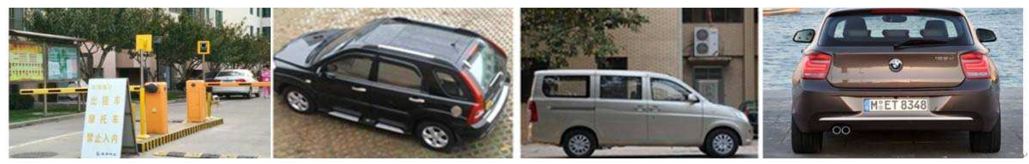
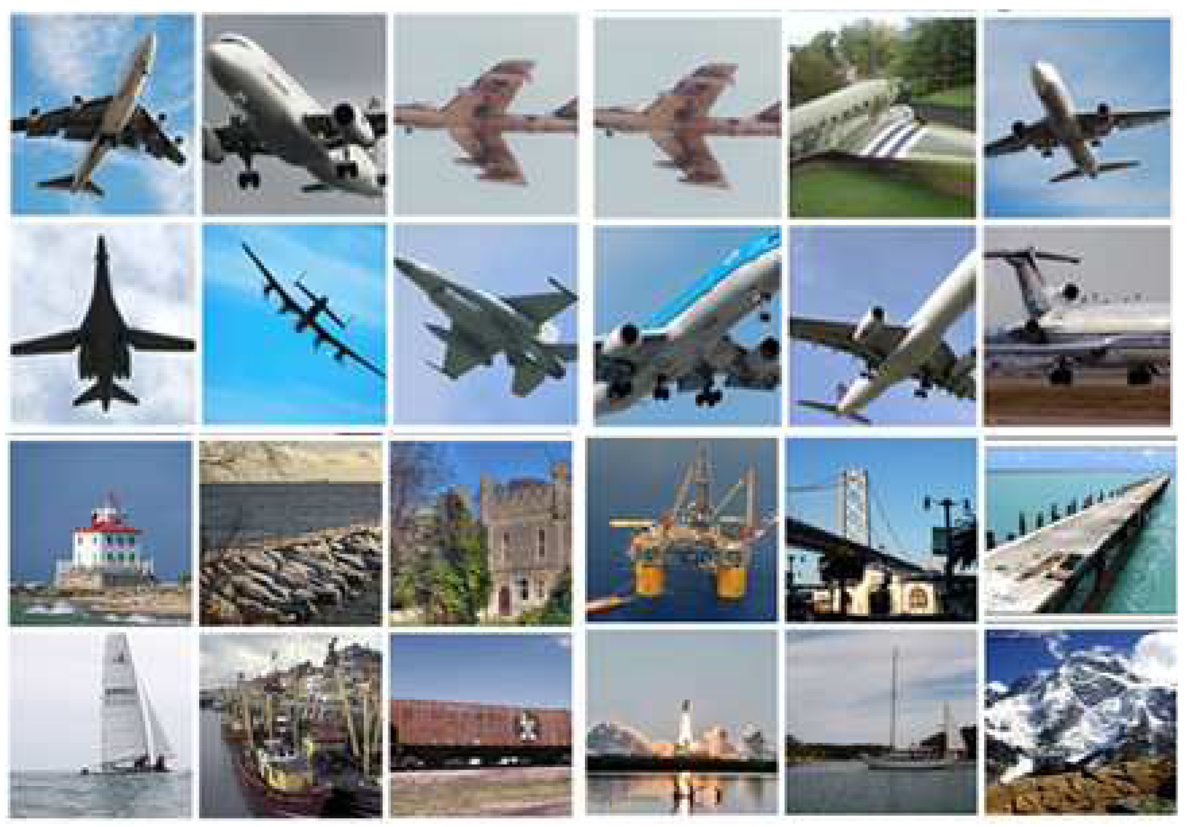
The data used in the transfer learning of objNet network were mainly extracted from the ImageNet 2012 dataset, in which positive samples were all images in two categories of airplane and military airplane and some airplane images crawled from the Internet, a total of 12,300 images; for negative samples, we picked a category that may appear in the remote sensing images, such as ships, harbors, mountains, etc., and removed the other 980 categories, such as sharks, hens, caps, etc., which might be useless for object identification in remote sensing images. Figure 17 shows examples of the positive and negative samples of the dataset. For the convenience of the following description, this dataset is called NATURE-PLANE.

5.5.2. Environment and Evaluation

The experiment in this section was performed on Caffe. Caffe is widely used in the deep learning domain because of its advantages of being clear, simple, fast, and fully open source. The platform had two NVIDIA GeForce GTX 980 video cards, 16 GB memory, CPU i5-4460. For a detection result with IoU overlap with a real object coincidence degree no less than a threshold (usually set to 0.5), the detection result is considered correct; besides, if there are multiple detections, then only one is considered right, while the rest are false detections. In this paper, we used the precision and recall curve (PR curve) and the average precision (AP) to evaluate the detection performance synthetically. The evaluation method and code used the PASCAL VOC2007 standard. Accuracy and recall are defined as Formulas (17) and (18), respectively:
P = T P T P + F P
R = T P T P + F N
where T P is true positive, the number of true boxes, that is the number of objects correctly detected; F P is false positive, the number of false positives, that is the number of false detection results; F N is false negative, the number of false negative cases, that is the true number of objects that were missed.
The average detection accuracy of A P can be measured by a single value, which is a representative comprehensive evaluation of the index, called the area under the P R curve, as shown in Formula (19).
A P = 0 1 P R d R
I o U = D e t e c t i o n R e s u l t G r o u n d T r u t h D e t e c t i o n R e s u l t G r o u n d T r u t h

5.5.3. Result Analysis

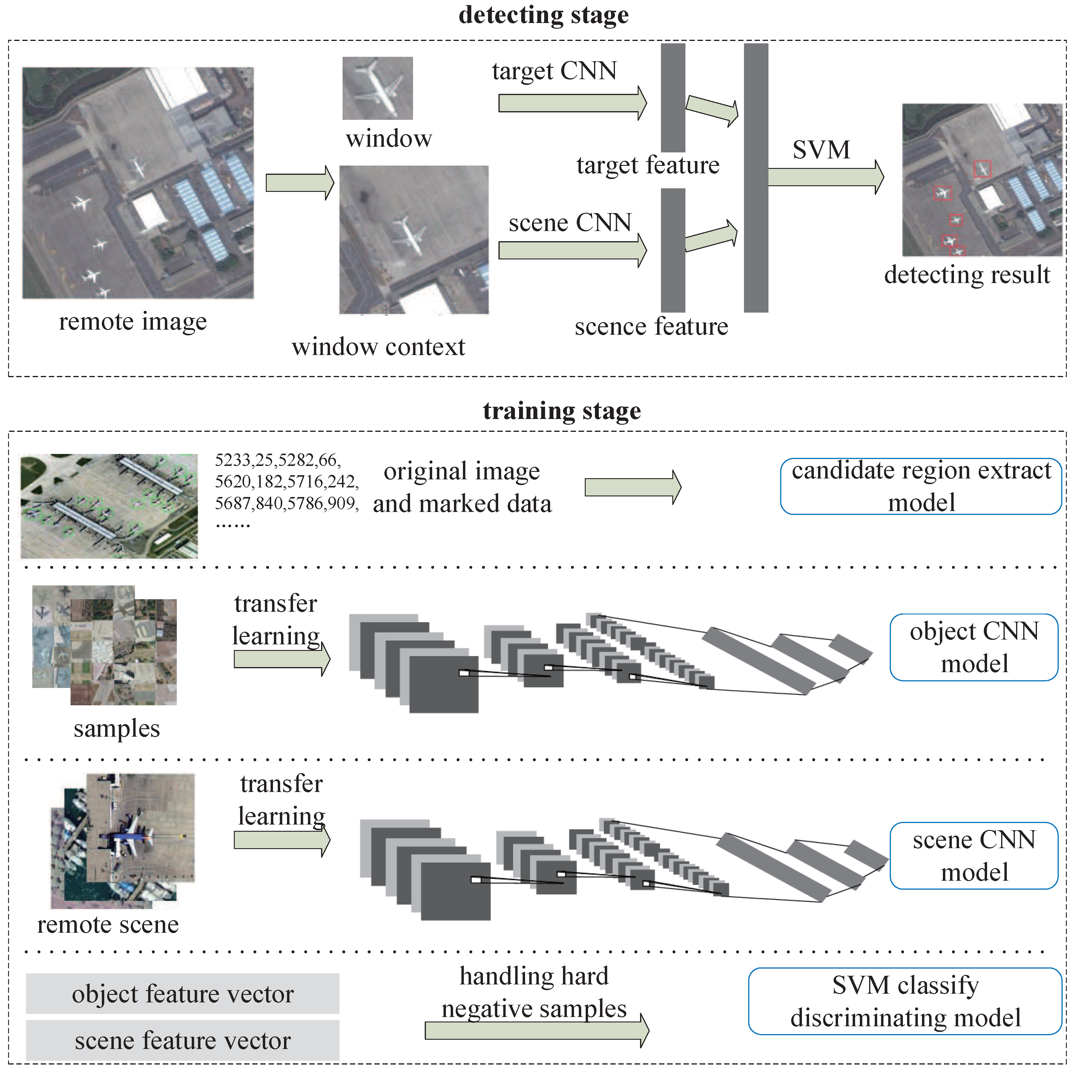
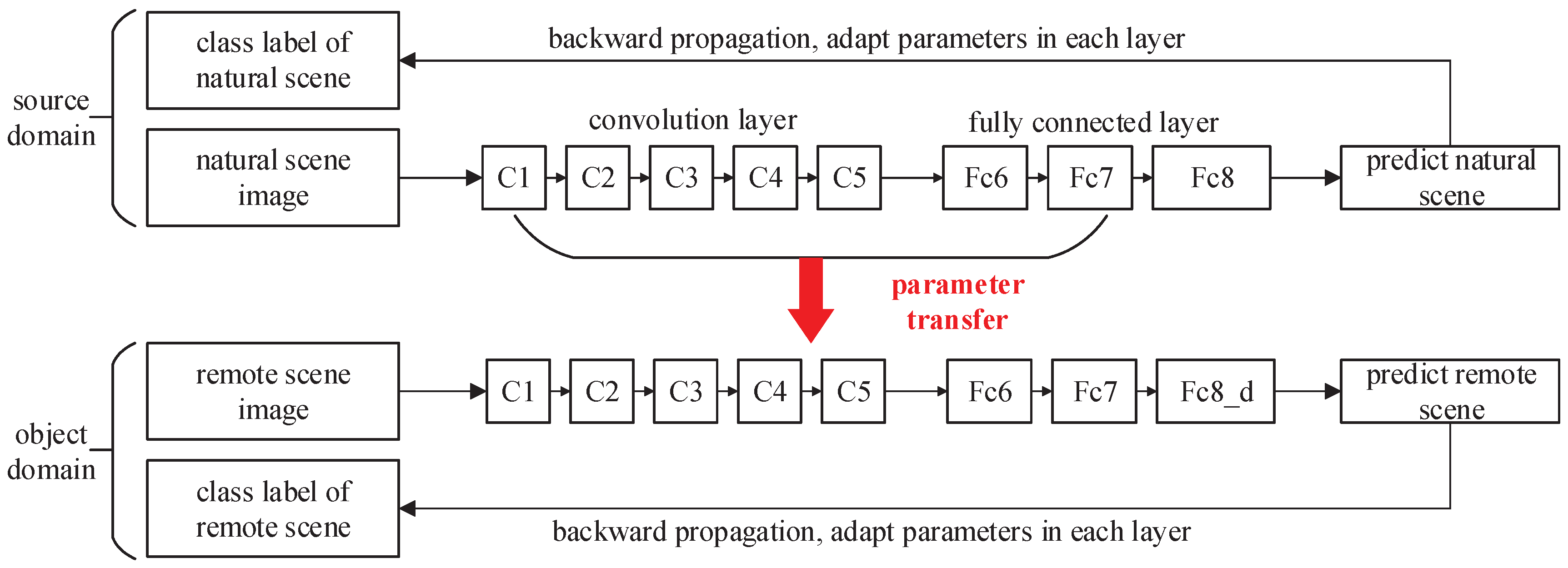
In order to prove the validity of the transfer learning, this section firstly gives the classification accuracy of the object and scene feature extraction network in the training process and then gives the influence of the feature extraction on the detection effect before and after the transfer learning. Furthermore, the effectiveness of scene feature fusion is illustrated by contrasting the detection performance before and after the context scene feature fusion. Finally, we compare the other algorithms to prove the validity of the proposed remote sensing object detection algorithm based on deep learning with scene feature fusion.
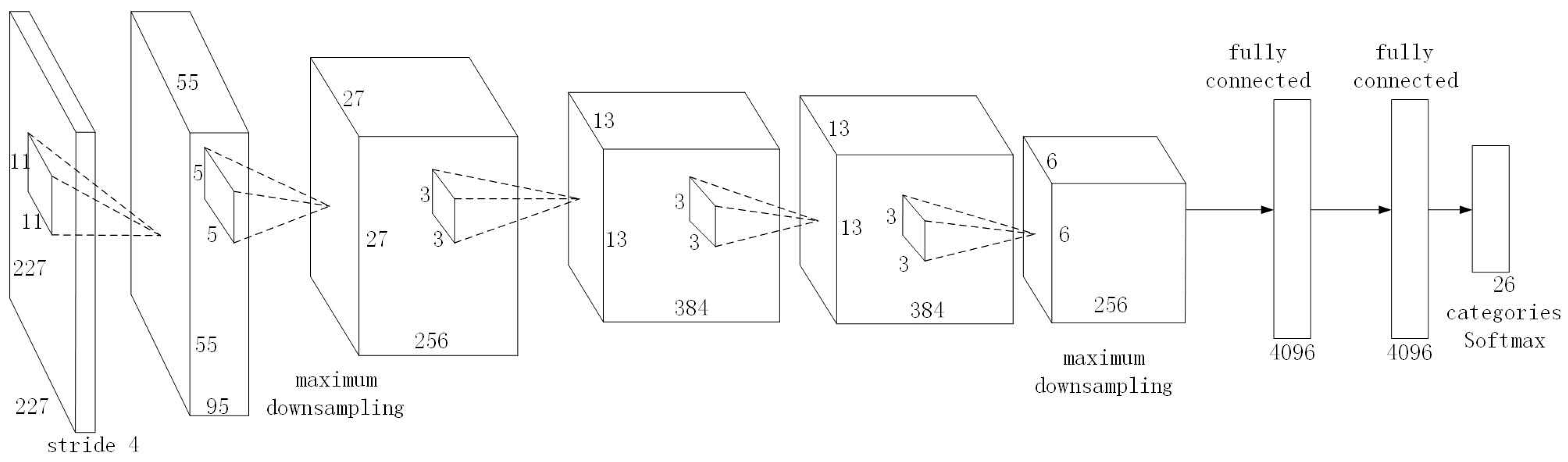
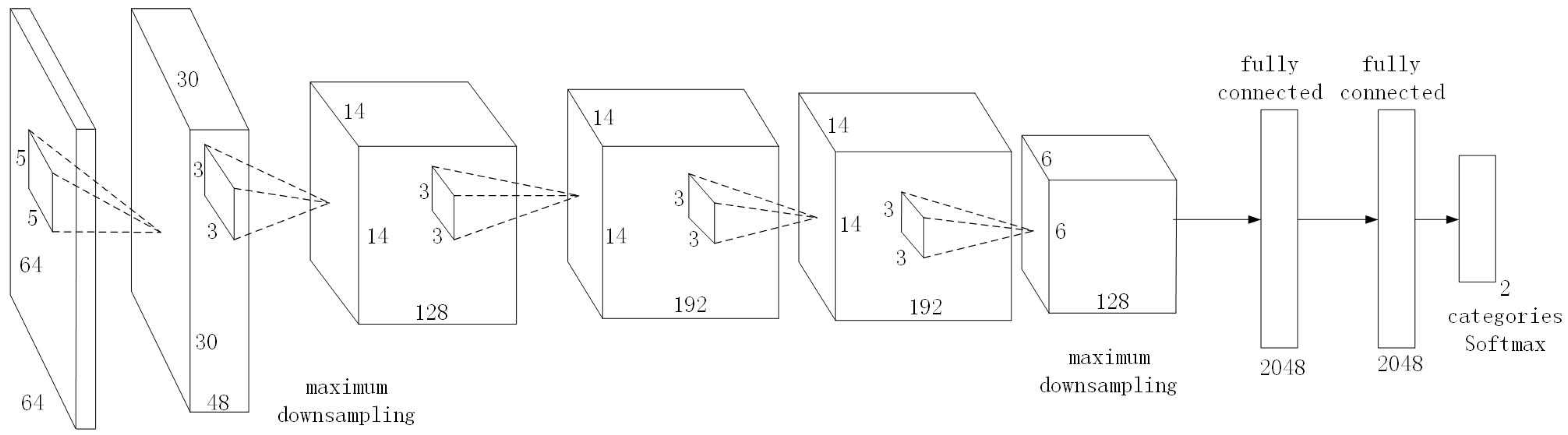
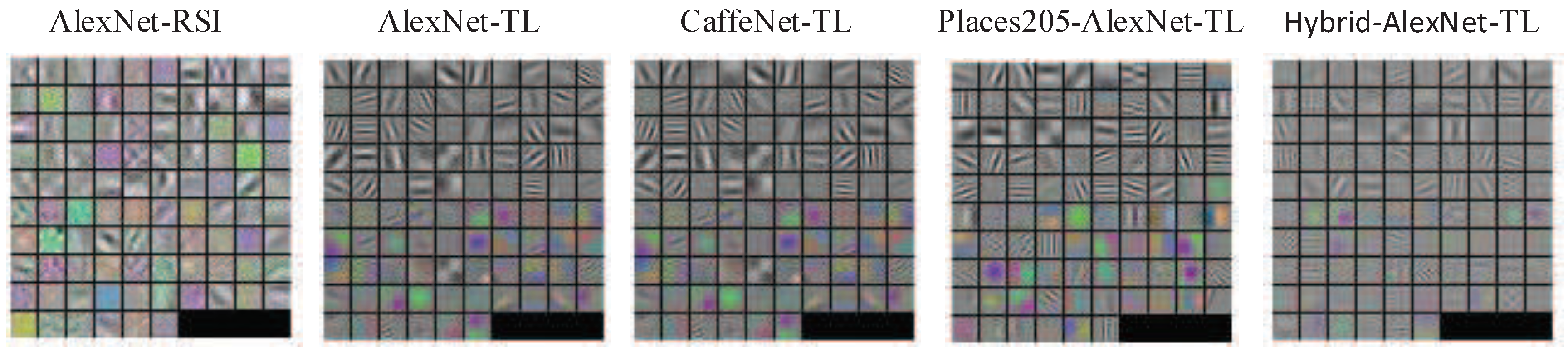
Because the sceNet network uses the classic AlexNet network structure, there are many trained parameter models based on the network, which can be used for transfer learning. During the training process, the parameter models of AlexNet, CaffeNet, Places205-AlexNet, and Hybrid-AlexNet were used for transfer learning in this paper. AlexNet and CaffeNet were trained on the ImageNet2012 dataset, and CaffeNet has a very similar architecture to AlexNet, except for two small modifications: training without data augmentation and exchanging the order of pooling and normalization layers. Places205-AlexNet is a parameter model trained on the Places dataset. Hybrid-AlexNet was trained on the dataset combining the Place dataset with the ImageNet2012 dataset for a total of 3.6 million images in 1183 categories. Table 5 shows the classification accuracy of the remote sensing scene using different transfer learning models, where “AlexNet-RSI” indicates the learned network model without transfer learning and “xx-TL” denotes the network transferred from different models.
Table 5 reveals that the accuracy of the network trained with transfer learning was much higher than that of a network trained directly using remote sensing scene data. After transfer learning, the accuracy of the Hybrid-AlexNet network trained on the Place and ImageNet 2012 datasets was the highest, so we used the Hybrid-AlexNet-TL model to extract the feature of the object context scene. In addition, by visualizing the convolution kernel parameters of the first convolution layer, as shown in Figure 18, this shows that the convolution kernel of the network with transfer learning learned more edge features, and without transfer learning, the first layer of the network simply learned some simple fuzzy color information.
For the training of object classification network objNet, because the network structure was designed in this paper, there was no trained model for transfer learning, so it was necessary to pre-train the transferable model parameters. Therefore, we used the NATURE-PLANE dataset introduced in Section 5.4.1 to pre-train objNet. However, in practice, it appears that if we pre-train the objNet directly using ImageNet2012’s complete data and resume training using the NATURE-PLANE dataset, a better classification result could be obtained. Table 6 lists the classification accuracy of different pre-trained objNet networks, where objNet-RSI denotes the network model obtained without using transfer learning.
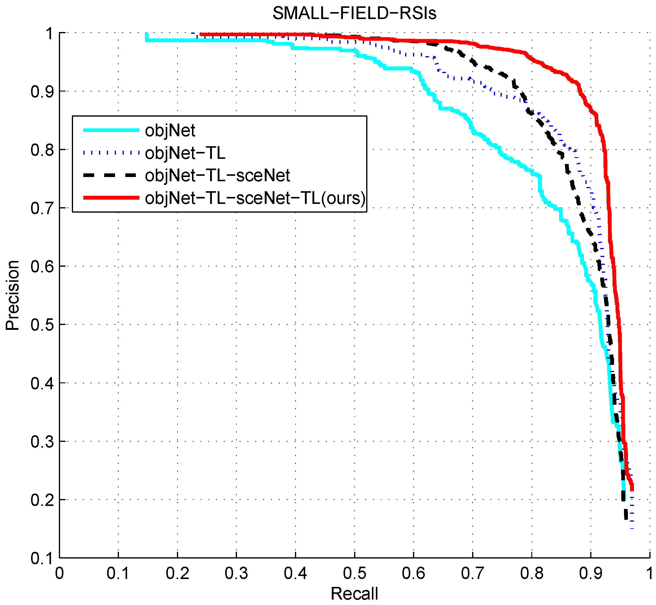
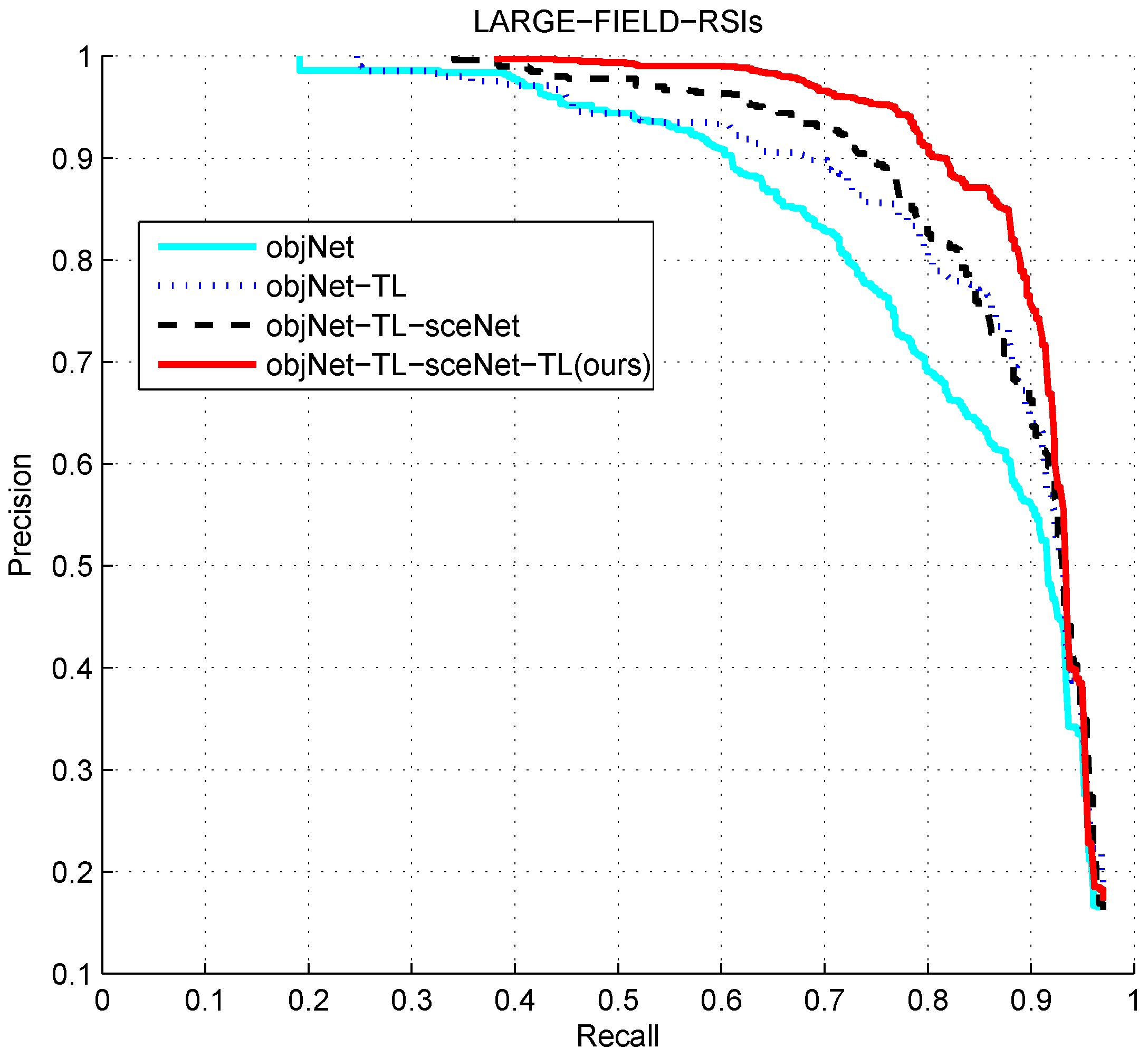
After the training of the objNet network and sceNet network was complete, we used the two networks for feature extraction and classification detection. We first compared the detection performance before and after using transfer learning in objNet when there was no scene feature fusion. Then, to fuse the scene features, in the fusion, we also compared the effect of sceNet before and after transfer. That is, there was in total four groups of experiments, and the four groups of experiments had a progressive relationship, in which the fourth set of experiments was our proposed algorithm. In order to simplify the following description, we named each experiment and the configuration of each set of experiments as listed in Table 7.
Figure 19 and Figure 20 show the comparison of the results of the four experiments on two different dataset sizes. From the results of the experiments objNet and objNet-TL, it was revealed that the transfer learning of object the feature extraction network could improve the whole detection performance significantly. Before transfer learning, the accuracy of the curve decreased rapidly with the recall increasing, and the curve decreased slowly after transfer learning, which shows that the extracted feature of network after transfer learning made the classifier discriminate better, which means the transfer learning was effective. It can be concluded from the experiment objNet-TL-sceNet-TL that the detection efficiency on the two remote sensing datasets was better than that for the experiment without context scene feature fusion, indicating the effectiveness of the scene feature fusion. However, compared with objNet-TL-sceNet and objNet-TL, it is shown that when transfer learning was not employed, the improvement was not obvious, the possible reason for which being that the sceNet network has too many parameters for the limited remote sensing scene data, and if we directly trained the network using limited data without transfer learning, it would easily to over-fit, so that the extracted features would not be representative.
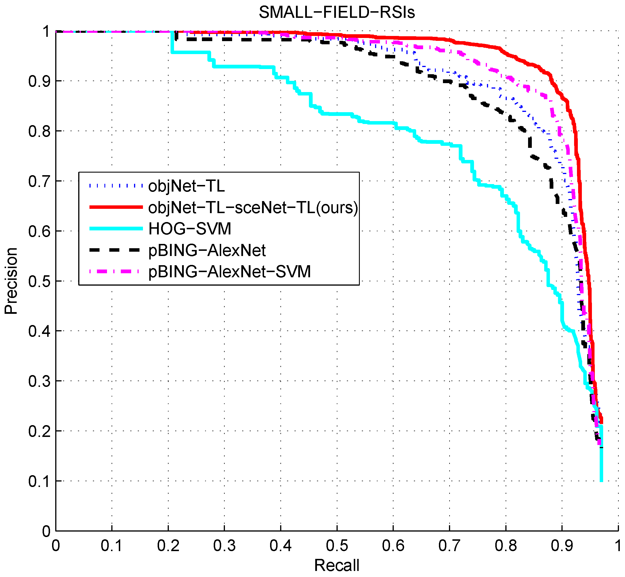
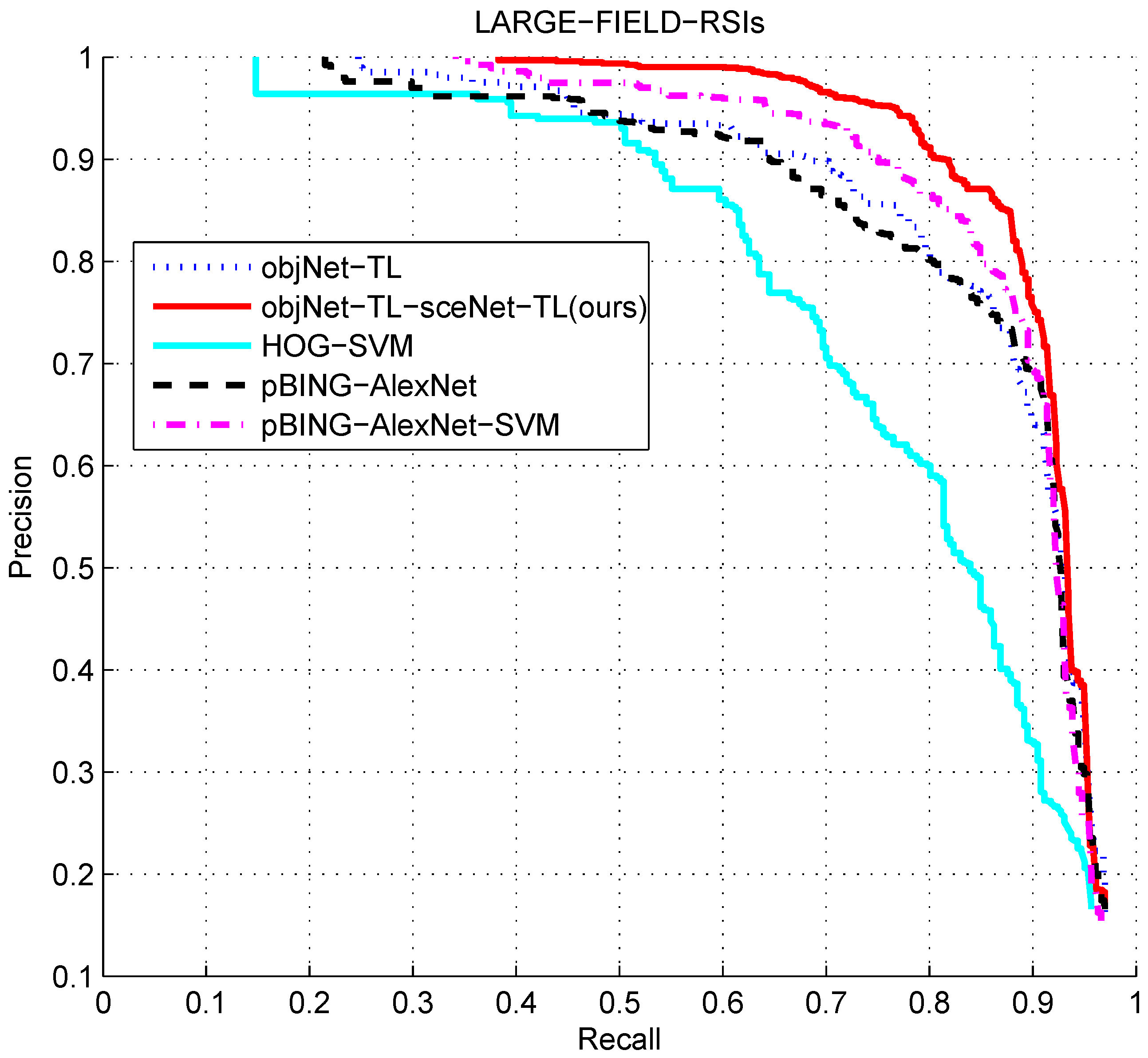
Finally, we compared the proposed algorithm objNet-TL-sceNet-TL with the other algorithms. Firstly, in order to prove the effectiveness of the deep features, we used the HOG algorithm [34] to extract the feature of the candidate region and used the SVM algorithm and the hard negative mining method to train the detector; we called it HOG-SVM. In addition, this paper compared the R-CNN algorithm [14]. This algorithm achieved a breakthrough in the PASCAL VOC2007 object detection task. It first uses the selective search algorithm to generate about 2000 candidate regions for each image and then uses the AlexNet network to extract features, and finally classifies each region using linear SVM classification. From the analysis of 
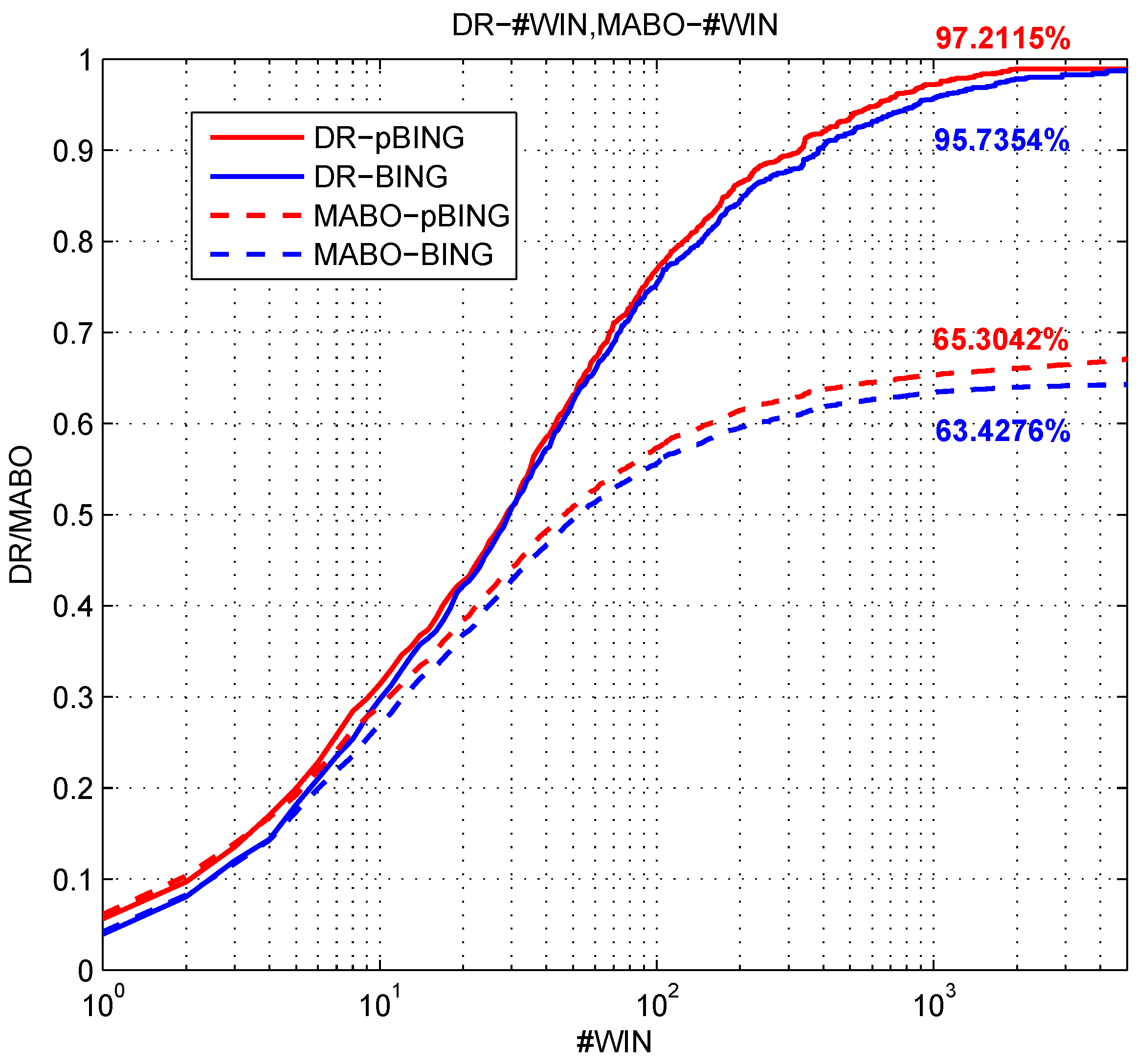
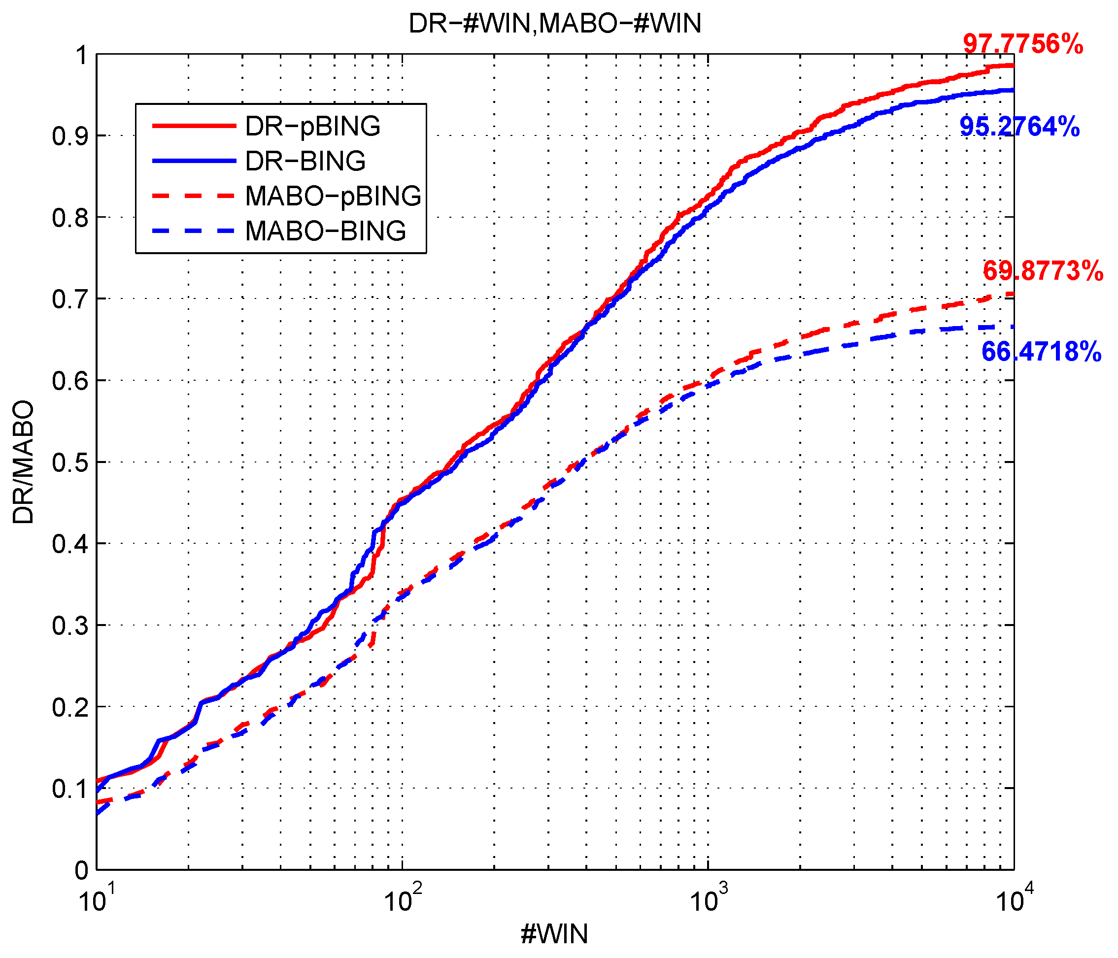
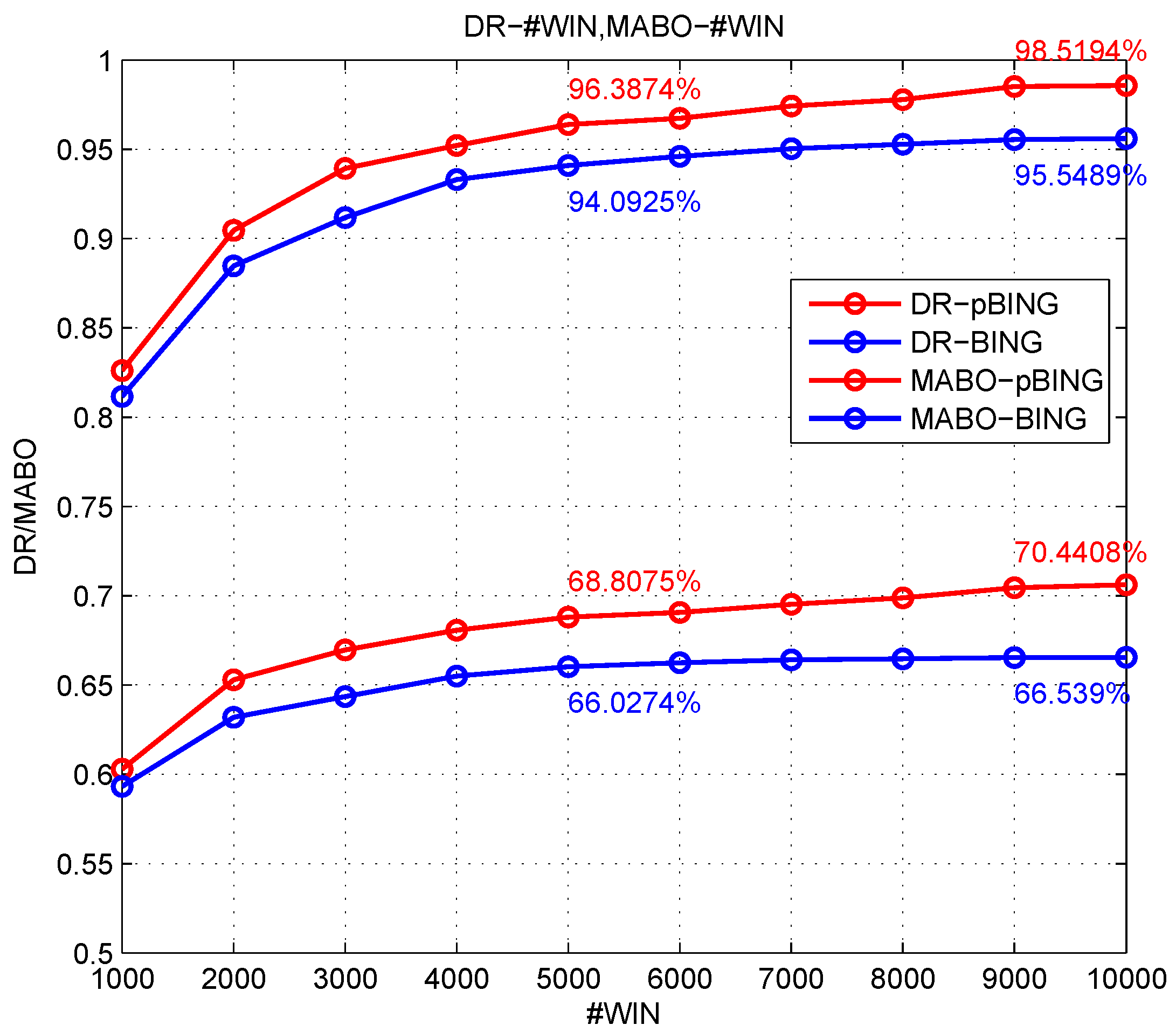
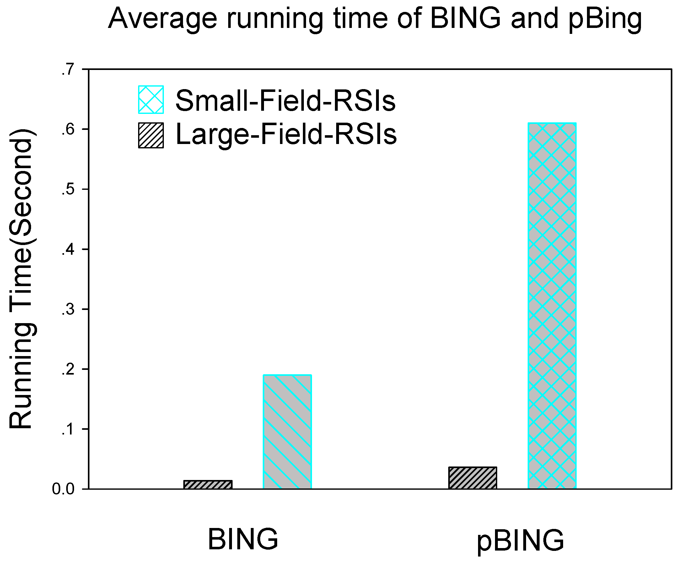
Section 4.3.2, we can see that the selective search algorithm is not suitable for large-sized remote sensing images. Therefore, this paper replaced the candidate region proposal with the pBING algorithm proposed in this paper. Furthermore, we compared the detection performance of the two methods of R-CNN: directly obtaining classification results by the AlexNet network and extracting features by AlexNet, then classifying by SVM. For convenience, the two algorithms are called pBING-AlexNet and pBING-AlexNet-SVM, respectively. Figure 21 and Figure 22 show the comparison of the detection performance of each algorithm on two different sizes of remote sensing images.
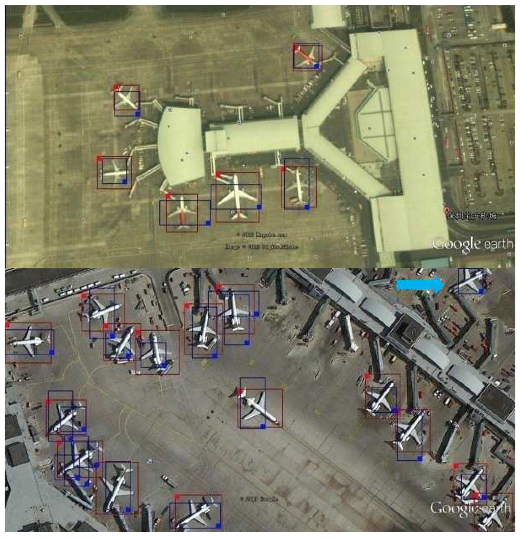
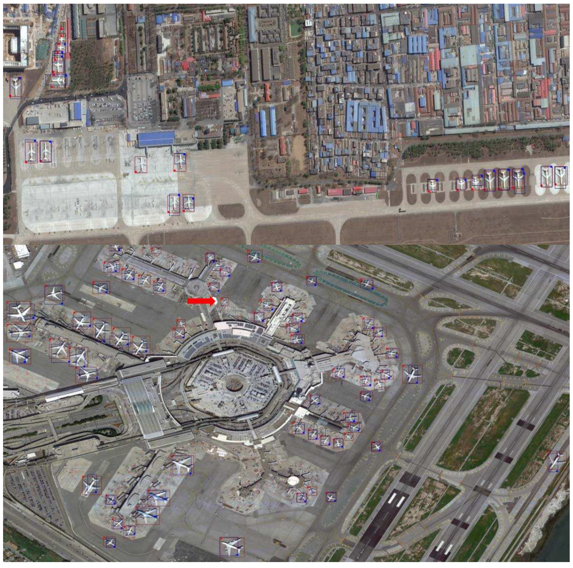
Figure 23 and 
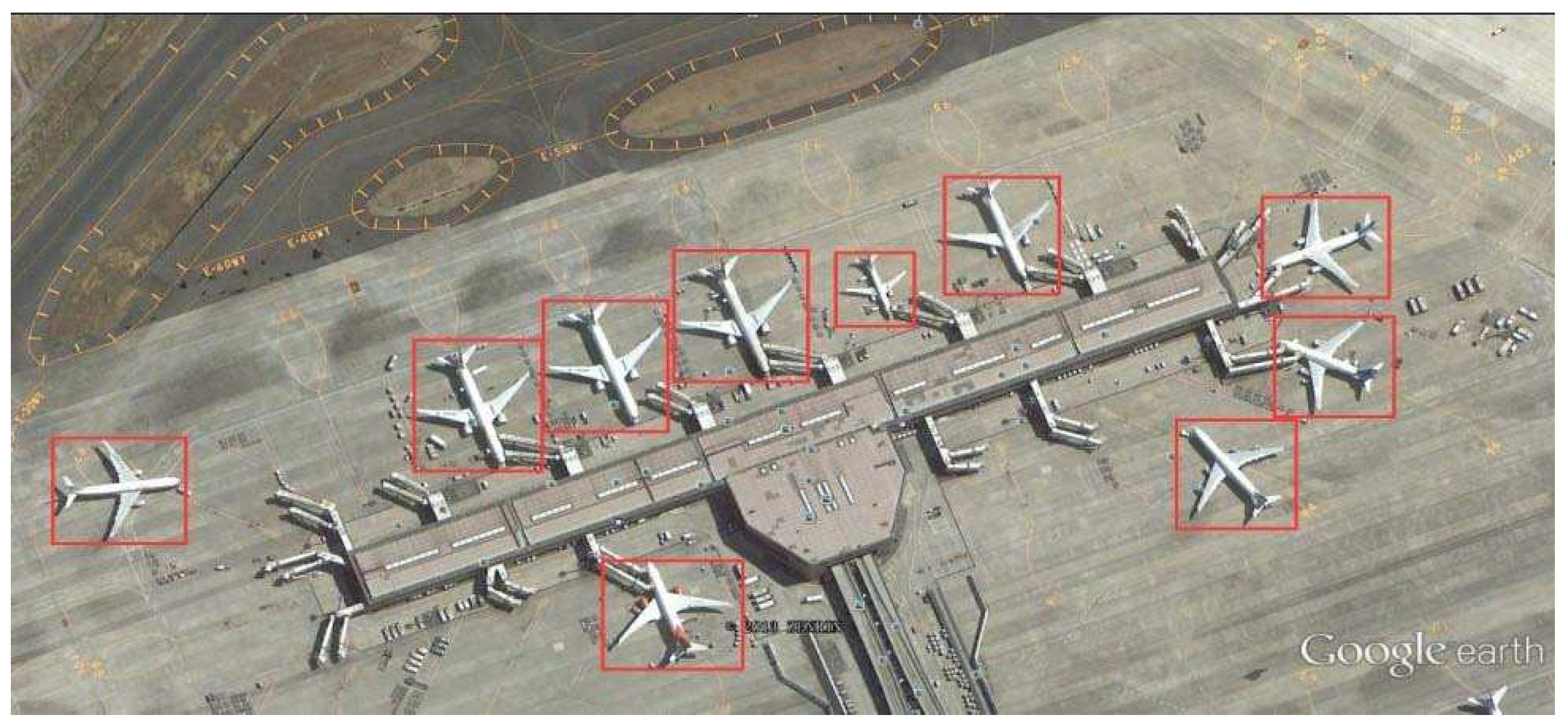
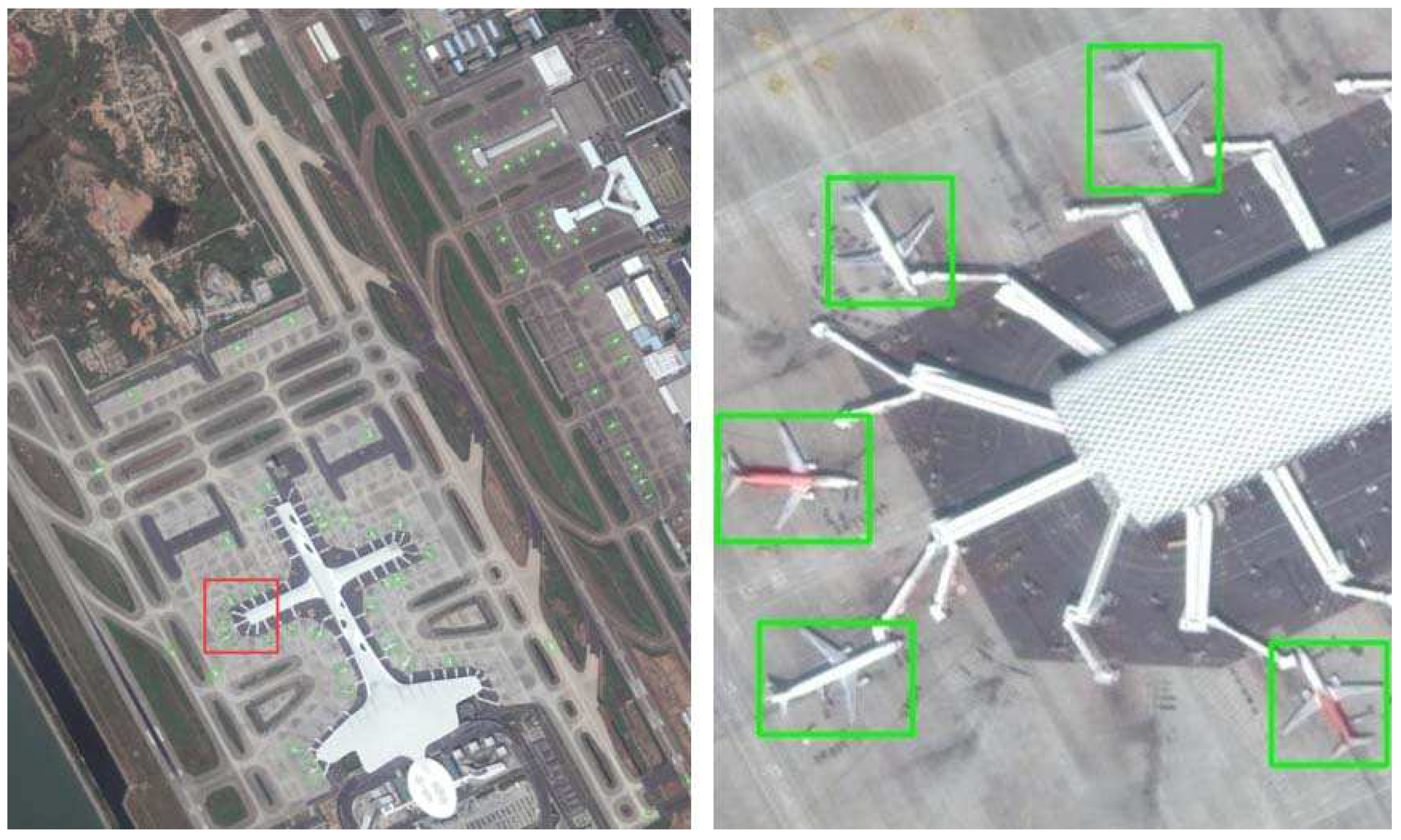
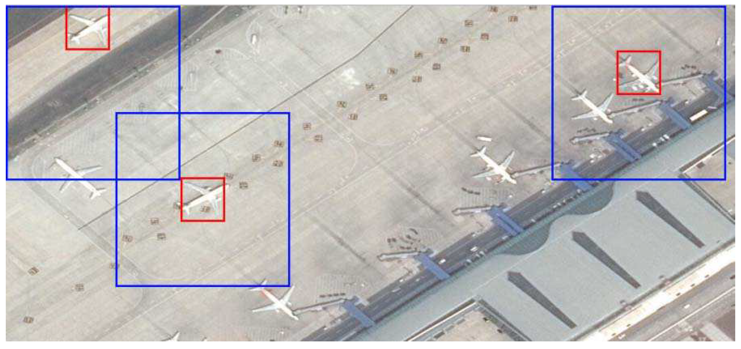
Figure 24 show the results of the objNet-TL-sceNet-TL algorithm on the SMALL-FIELD-RSIs and LARGE-FIELD-RSIs datasets, respectively. In each image, the red rectangles indicate the real objects marked by the dataset and the blue rectangles the final detection result of our algorithm. It appears that the vast majority of airplane objects can be correctly detected. It is noted that our algorithm can detect one airplane, which was not marked (missed by a human) on the dataset, and it is shown by the blue arrow in Figure 23. The comparison details of average precision (AP) can be checked in Table 8.
However, we found that if the airplane object was ambiguous and small, it may be missed. One missed airplane is pointed out by the red arrow in Figure 24. The reason is that our candidate region proposal algorithm was not strong enough for objects that are too small and ambiguous, and it needs to be further improved in the future.

6. Conclusions

In this paper, we present a deep fusion feature approach to detect objects in high-resolution remote sensing images. Our method is composed of three main steps, which are the candidate region generation, deep feature extraction with fine-tuning, and the SVM classification with deep features. Hence, we re-structured the paper in terms of the three steps. For candidate region generation, we improved the binarized normed gradients algorithm and developed the pBING method. For deep feature extraction, the object feature and scene feature were both extracted for each candidate region, by utilizing the AlexNet model. As the label data in remote sensing are very scarce, we utilized the fine-tuning notion and pre-trained AlexNet on the ImageNet database, then fine-tuned the model with labeled remote sensing data. Finally, the object feature and scene feature were utilized to train an SVM for classification. After introducing the three main steps, we reported the experimental results, which validated the effectiveness of the developed pBING method, the fine-tuning strategy, and the overall detection model.

Author Contributions

E.K.W. is the main writer of the paper. Y.L. responds to the algorithms. Z.N. responds to design the pBing algorithm, J.Y., Z.L. and X.Z. respond to make experiments. S.M.Y. responds to the English Check.

Funding

This research was supported in part by the National Natural Science Foundation of China (No. 61572157), Grant No. 2016A030313660 and 2017A030313365 from the Guangdong Province Natural Science Foundation, and JCYJ20160608161351559, KQJSCX70726103044992, JCYJ20170811155158682, and JCYJ20160428092427867 from the Shenzhen Municipal Science and Technology Innovation Project. The authors thank the reviewers for their comments.

Conflicts of Interest

The authors declare no conflicts of interest.

References

  1. Weber, J.; Lefevre, S. A multivariate hit-or-miss transform for conjoint spatial and spectral template matching. In Proceedings of the International Conference on Image and Signal Processing, Cherbourg-Octeville, France, 1–3 July 2008; pp. 226–235. [Google Scholar]
  2. Sirmacek, B.; Unsalan, C. Urban-area and building detection using SIFT keypoints and graph theory. IEEE Trans. Geosci. Remote Sens. 2009, 47, 1156–1167. [Google Scholar] [CrossRef]
  3. Yokoya, N.; Iwasaki, A. Object localization based on sparse representation for remote sensing imagery. In Proceedings of the International Geoscience and Remote Sensing Symposium, Quebec City, QC, Canada, 13–18 July 2014; pp. 2293–2296. [Google Scholar]
  4. Tao, C.; Tan, Y.; Cai, H.; Tian, J. Airport detection from large ikonos images using clustered sift keypoints and region information. IEEE Geosci. Remote Sens. Lett. 2011, 8, 128–132. [Google Scholar] [CrossRef]
  5. Sun, H.; Sun, X.; Wang, H.; Li, Y.; Li, H. Automatic target detection in high-resolution remote sensing images using spatial sparse coding bag-of-words mode. IEEE Geosci. Remote Sens. Lett. 2012, 9, 109–113. [Google Scholar] [CrossRef]
  6. Gan, L.; Liu, P.; Wang, L. Rotation sliding window of the hog feature in remote sensing images for ship detection. In Proceedings of the 8th International Symposium on Computational Intelligence and Design, Hangzhou, China, 12–13 December 2015; pp. 401–404. [Google Scholar]
  7. Arastounia, M.; Oude Elberink, S. Application of template matching for improving classification of urban railroad point clouds. Sensors 2016, 16, 2112. [Google Scholar] [CrossRef] [PubMed]
  8. Aytekin, O.; Zongur, U.; Halici, U. Texture-based airport runway detection. IEEE Geosci. Remote Sens. Lett. 2013, 10, 471–475. [Google Scholar] [CrossRef]
  9. Felzenszwalb, P.F.; Girshick, R.B.; McAllester, D.; Ramanan, D. Object detection with discriminatively trained part-based models. IEEE Trans. Pattern Anal. Mach. Intell. 2010, 32, 1627–1645. [Google Scholar] [CrossRef]
  10. Han, J.; Zhang, D.; Cheng, G.; Guo, L.; Ren, J. Object detection in optical remote sensing images based on weakly supervised learning and high-level feature learning. IEEE Trans. Geosci. Remote Sens. 2015, 53, 3325–3337. [Google Scholar] [CrossRef]
  11. Mottaghi, R.; Chen, X.; Liu, X.; Cho, N.-G.; Lee, S.-W.; Fidler, S.; Urtasun, R.; Yullie, A. The role of context for object detection and semantic segmentation in the wild. In Proceedings of the IEEE Conference on Computer Vision and Pattern Recognition, Columbus, OH, USA, 23–28 June 2014; pp. 891–898. [Google Scholar]
  12. Ren, X.; Ramanan, D. Histograms of sparse codes for object detection. In Proceedings of the IEEE Conference on Computer Vision and Pattern Recognition, Portland, OR, USA, 23–28 June 2013; pp. 3246–3253. [Google Scholar]
  13. Krizhevsky, A.; Sutskever, I.; Hinton, G.E. Imagenet Classification with Deep CNNs. In Proceedings of the Advances in Neural Information Processing Systems, Lake Tahoe, NV, USA, 3–6 December 2012; pp. 1097–1105. [Google Scholar]
  14. Uijlings, J.; Sande, K.E.; Gevers, T.; Smeulders, A.W.M. Selective search for object recognition. Int. J. Comput. Vis. 2013, 104, 154–171. [Google Scholar] [CrossRef]
  15. Cheng, M.; Zhang, Z.; Lin, W.-Y.; Torr, P. BING: Binarized Normed Gradients for Objectness Estimation at 300fps. In Proceedings of the Computer Vision and Pattern Recognition, Columbus, OH, USA, 24–27 June 2014; pp. 3286–3293. [Google Scholar]
  16. Zitnick, C.L.; Dollar, P. Edge boxes: Locating object proposals from edges. In Proceedings of the European Conference on Computer Vision, Zurich, Switzerland, 6–12 September 2014; pp. 391–405. [Google Scholar]
  17. Humayun, A.; Li, F.; Rehg, J.M. RIGOR: Reusing inference in graph cuts for generating object regions. In Proceedings of the Computer Vision and Pattern Recognition, Columbus, OH, USA, 24–27 June 2014; pp. 336–343. [Google Scholar]
  18. Girshick, R.; Donahue, J.; Darrell, T.; Malik, J. Rich feature hierarchies for accurate object detection and semantic segmentation. In Proceedings of the Computer Vision and Pattern Recognition, Columbus, OH, USA, 24–27 June 2014; pp. 580–587. [Google Scholar]
  19. Simonyan, K.; Zisserman, A. Very deep convolutional networks for large-scale image recognition. arXiv, 2014; arXiv:1409.1556. [Google Scholar]
  20. Oquab, M.; Bottou, L.; Laptev, I.; Sivic, J. Learning and transferring mid-level image representations using convolutional neural networks. In Proceedings of the IEEE Computer Vision and Pattern Recognition, Columbus, OH, USA, 24–27 June 2014; pp. 1717–1724. [Google Scholar]
  21. Girshick, R.; Donahue, J.; Darrell, T.; Malik, J. Region-based convolutional networks for accurate object detection and segmentation. IEEE Trans. Pattern Anal. Mach. Intell. 2016, 38, 142–158. [Google Scholar] [CrossRef] [PubMed]
  22. Kong, T.; Yao, A.; Chen, Y.; Sun, F. HyperNet: Towards Accurate Region Proposal Generation and Joint Object Detection. Accurate region proposal generation and joint object detection. In Proceedings of the Computer Vision and Pattern Recognition, Las Vegas, NV, USA, 26 June–1 July 2016; pp. 845–853. [Google Scholar]
  23. Ouyang, W.; Wang, X.; Zeng, X.; Qiu, S.; Luo, P.; Tian, Y.; Li, H.; Yang, S.; Wang, Z.; Loy, C.-C.; et al. DeepID-Net: Deformable deep convolutional neural networks for object detection. In Proceedings of the Computer Vision and Pattern Recognition, Boston, MA, USA, 7–12 June 2015; pp. 2403–2412. [Google Scholar]
  24. Redmon, J.; Divvala, S.; Girshick, R.; Farhadi, A. You only look once: Unified, real-time object detection. In Proceedings of the Computer Vision and Pattern Recognition, Boston, MA, USA, 7–12 June 2015; pp. 779–788. [Google Scholar]
  25. Hosang, J.; Benenson, R.; Dollar, P.; Schiele, B. What makes for effective detection proposals? IEEE Trans. Pattern Anal. Mach. Intell. 2016, 38, 814–830. [Google Scholar] [CrossRef] [PubMed]
  26. Hare, S. Efficient online structured output learning for keypoint-based object tracking. In Proceedings of the IEEE Conference on Computer Vision and Pattern Recognition, Providence, RI, USA, 16–21 June 2012; pp. 1894–1901. [Google Scholar]
  27. Zheng, S.; Sturgess, P.; Torr, P.H.S. Approximate structured output learning for constrained local models with application to real-time facial feature detection and tracking on low-power devices. In Proceedings of the IEEE International Conference and Workshops on Automatic Face and Gesture Recognition, Shanghai, China, 22–26 April 2013; pp. 1–8. [Google Scholar]
  28. Kegl, B. The return of AdaBoost.MH: Multi-class hamming trees. arXiv, 2013; arXiv:1312.6086. [Google Scholar]
  29. Wang, X.; Han, T.X.; Yan, S. An HOG-LBP human detector with partial occlusion handling. In Proceedings of the International Conference on Computer Vision, Lisboa, Portugal, 5–8 February 2009; pp. 32–39. [Google Scholar]
  30. Srivastava, N.; Hinton, G.; Krizhevsky, A.; Sutskever, I.; Salakhutdinov, R. Dropout: A simple way to prevent neural networks from overfitting. J. Mach. Learn. Res. 2014, 15, 1929–1958. [Google Scholar]
  31. Zhou, B.; Garcia, A.L.; Xiao, J.; Torralba, A.; Olivia, A. Learning deep features for scene recognition using places database. In Proceedings of the Advances in Neural Information Processing Systems, Montreal, QC, Canada, 7–12 December 2015; pp. 487–495. [Google Scholar]
  32. Yang, Y.; Newsam, S. Bag-of-visual-words and spatial extensions for land-use classification. In Proceedings of the Advances in Geographic Information Systems, San Jose, CA, USA, 2–5 November 2010; pp. 270–279. [Google Scholar]
  33. Xia, G.S.; Yang, W.; Delon, J.; Gousseau, Y.; Sun, H.; Maitre, H. Structural high-resolution satellite image indexing. In Proceedings of the ISPRS TC VII Symposium-100 Years ISPRS, Vienna, Austria, 5–7 July 2010; pp. 298–303. [Google Scholar]
  34. Dalal, N.; Triggs, B. Histograms of oriented gradients for human detection. In Proceedings of the Computer Vision and Pattern Recognition, San Diego, CA, USA, 20–25 June 2005; pp. 886–893. [Google Scholar]
Figure 1. Proposed object detection framework.
Applsci 09 01130 g001
Figure 2. pBING algorithm flowchart.
Applsci 09 01130 g002
Figure 3. The annotation method of the airplane object.
Applsci 09 01130 g003
Figure 4. The high-resolution remote sensing image of Baoan Airport.
Applsci 09 01130 g004
Figure 5. Tradeoff between the number of windows (#WIN) and DR/MABO on the dataset SMALL-FIELD-RSIs.
Applsci 09 01130 g005
Figure 6. Tradeoff between #WIN and the detection rate (DR)/mean average best overlap (MABO) on the dataset LARGE-FIELD-RSIs.
Applsci 09 01130 g006
Figure 7. Tradeoff between #WIN and DR/MABO on the dataset LARGE-FIELD-RSIs when #WIN varied from 1000–10,000.
Applsci 09 01130 g007
Figure 8. Average running time of the BING algorithm and the pBING algorithm on different datasets.
Applsci 09 01130 g008
Figure 9. Example of the context scene of a car in regular images.
Applsci 09 01130 g009
Figure 10. Airplane objects in high-resolution remote sensing images.
Applsci 09 01130 g010
Figure 11. Window feature and context scene feature fusion.
Applsci 09 01130 g011
Figure 12. The definition of the context scene for the candidate region.
Applsci 09 01130 g012
Figure 13. sceNet network structure.
Applsci 09 01130 g013
Figure 14. objNet network structure.
Applsci 09 01130 g014
Figure 15. The training process of CNN.
Applsci 09 01130 g015
Figure 16. The transfer learning flowchart of the sceNet network.
Applsci 09 01130 g016
Figure 17. Examples of the NATURE-PLANE dataset used in the transfer learning of the objNet network.
Applsci 09 01130 g017
Figure 18. Visualization of the first-level convolutions in different network models.
Applsci 09 01130 g018
Figure 19. The performance comparison of four experiments on the SMALL-FIELD-RSIs dataset.
Applsci 09 01130 g019
Figure 20. The performance comparison of four experiments on the LARGE-FIELD-RSIs dataset.
Applsci 09 01130 g020
Figure 21. The performance comparison of different algorithms on the SMALL-FIELD-RSIs dataset.
Applsci 09 01130 g021
Figure 22. The performance comparison of different algorithms on the LARGE-FIELD-RSIs dataset.
Applsci 09 01130 g022
Figure 23. Examples of detection results on the SMALL-FIELD-RSI dataset.
Applsci 09 01130 g023
Figure 24. Examples of detection results on the LARGE-FIELD-RSIs dataset.
Applsci 09 01130 g024
Table 1. The experimental dataset.
Dataset NameSpatial ResolutionImage Size (Pixels)Number of ImagesNumber of Objects
SMALL-FIELD-RSIs0.6 m1300 × 8009807452
LARGE-FIELD-RSIs0.6 m5000 × 50001093380
Table 2. The performance analysis for the selective search algorithm.
remote image scale (pixel)500 × 500800 × 8001000 × 10001500 × 1500
average number of candidate windows without constraints31617123906013,810
average number of candidate windows after filtering30396270846912,782
average computing time (s)2.77.614.329.8
Table 3. The parameters of each layer in the sceNet network.
1st Layer2nd Layer3rd Layer4th Layer5th Layer
convolution layerwindow size11 × 115 × 53 × 33 × 33 × 3
number of convolution kernels96256384384256
stride41111
pad02111
pooling layerwindow size3 × 33 × 33 × 3
stride222
Table 4. The parameters of each layer in objNet network.
1st Layer2nd Layer3rd Layer4th Layer5th Layer
convolution layerwindow size5 × 53 × 33 × 33 × 33 × 3
number of convolution kernels4812819219228
stride11111
pad00110
pooling layerwindow size2 × 22 × 22 × 2
stride222
Table 5. The classification accuracy of the network transferred from different models.
AlexNet-RSIAlexNet-TLCaffeNet-TLPlaces205 -AlexNet-TLHybrid -AlexNet-TL
accuracy89.76%94.04%93.87%92.68%94.81%
Table 6. The accuracy of objNet based on different transfer learning methods.
Accuracy
SMALL-FIELD-RSIsLARGE-FIELD-RSIs
objNet-RSI93.51%94.24%
objNet-TL196.63%95.52%
objNet-TL297.23%96.86%
Table 7. List pf the configurations of each experiment.
AlgorithmScene Feature FusionsceNet Transfer LearningobjNet Transfer Learning
objNet××
objNet-TL×
objNet-TL-sceNet×
objNet-TL-sceNet-TL (ours)
Table 8. The average detection accuracy (average precision (AP)).
AlgorithmSMALL-FIELD-RSIsLARGE-FIELD-RSIs
objNet83.38%82.30%
objNet-TL87.59%85.19%
objNet-TL-sceNet87.67%86.86%
objNet-TL-sceNet-TL (ours)90.77%89.12%
HOG-SVM77.52%76.69%
pBING-AlexNet85.63%84.54%
pBING-AlexNet-SVM88.93%86.91%

