Analysis and Design of A PMQR-Type Repetitive Control Scheme for Grid-Connected H6 Inverters


1
College of Information Engineering, Nanchang University, Nanchang 330031, China
2
Department of Electronics, Carleton University, Ottawa, ON K1S 5B6, Canada
*
Author to whom correspondence should be addressed.
Appl. Sci. 2019, 9(6), 1198; https://doi.org/10.3390/app9061198
Submission received: 27 February 2019
/
Revised: 11 March 2019
/
Accepted: 15 March 2019
/
Published: 21 March 2019
(This article belongs to the Section Energy Science and Technology)
Abstract
:There exist several challenges in the implementation of proportional multiple quasi-resonant (PMQR) control strategies in single-phase grid-connected H6 inverters, such as high computational costs and design complexity. To overcome these challenges, this paper proposes a proportional multiple quasi-resonant (PMQR)-type repetitive control (PMQR-type RC) scheme for single-phase grid-connected H6 inverters. In the control scheme, a repetitive controller and a proportional controller run in parallel. The repetitive controller is to improve the steady-state harmonics compensation ability, while the proportional controller can enhance the transient performance of the system. Both theoretical stability analysis and detailed design steps regarding the proposed control scheme are introduced. Finally, comparison results on a typical single-phase grid-connected H6 inverter with LC filter under a variety of control methods verify the capability of suppressing harmonics and the robust performance of the proposed control strategy against grid disturbances.
1. Introduction
Distributed power generation systems (DPGSs) based on renewable energy sources have been increasingly implemented world-wide, such as wind and solar energy [1]. The inverter configurations and corresponding current control strategies play an important roles in a grid-connected DPGS. Being a key interface equipment between a power generation source and the utility grid, the grid-tied inverter needs to ensure a high power conversion efficiency and guarantee the high-quality current injection into the grid. Typically, the output current total harmonic distortion (THD), which is a crucial index for assessing the power quality, must be less than 5% for both wind turbines and photovoltaic arrays connected to the grid [2]. In order to obtain a high-quality grid current and maintain a low output current THD value, researchers have proposed various current control strategies, such as PI control [3], proportional-repetitive (PR) control [4] and repetitive control [5].
Due to the absence of the transformer between the power generation source and utility grid to achieve galvanic isolation, there are potential power quality and safety issues in grid-connected inverters [6]. To tackle these issues, various inverter topologies have been designed [7,8]. For instance, full-bridge inverters are the most commonly used, which have a nice compromise among efficiency, complexity, and cost. However, this will generate relatively large common-mode leakage current, which increases the current harmonic content injected into grid and system loss. Half-bridge inverters with only two active switches are immune to leakage currents. However, this requires twice the input voltage of a full-bridge inverter. Practice has shown that adding more active switches to the full-bridge topology with a suitable PWM modulation strategy can achieve both high efficiency and low leakage current. The transformer-less H6 inverter, which features a simple structure, high efficiency, small ground leakage current, and low output current distortion, can be extensively used in the renewable energy power generation industry [9,10].
Various grid-tied current control techniques have been proposed to achieve the steady-state harmonics suppression. Among these control methods, the proportional-integral (PI) and proportional-repetitive (PR) control are popular methods [11,12,13,14]. The PI control scheme is commonly used in the stationary reference frame (SRF) for its simple control structure, ease of implementation, and good transient response [14]. However, a PI controller is unable to track a sinusoidal reference with zero steady-state error because of the limited control-loop gain [15]. It also lacks sufficient suppression ability for low frequency harmonics. On the other hand, the PR control technique, using the stationary reference frame, can efficiently overcome the aforementioned disadvantages of the PI control scheme. Thus, it possesses a high reputation in grid-connected control. The PR controller is composed of a proportional component like PI control and a resonant controller that acts as a sinusoidal integrator [12]. Theoretically, an ideal PR compensator introduces an infinite gain at resonant frequency, which is equal to grid frequency, to achieve a good sinusoidal reference current tracking effect. However, a PR controller will cause periodic disturbances at frequencies distinct from its resonant frequency and is unable to turn its control gain independently. The proportional multiple resonant control scheme together with its improved design can address the issue of multi-frequency harmonics compensation efficiently [16,17,18,19]. However, there is no doubt that multiple resonant (or quasi-resonant) controllers will lead to computational cost and significantly increase implementation complexity [20]. The repetitive controller (RC) has been presented with a simplified control structure, tracking many harmonics simultaneously. For the design of repetitive control, the control plant can be simplified as a single-input-single-output system. As a result, the design complexity is greatly reduced, and the stability assessment becomes easier. However, it cannot satisfy the requirements of dynamic response in renewable energy generation [21].
To address the issues mentioned above, this paper presents a proportional multiple quasi-resonant-type repetitive control (PMQR-type RC) scheme for single-phase grid-connected H6 inverters with the LC filter. The proposed controller consists of a proportional component and a repetitive controller in parallel, resulting in a better harmonics suppression performance and faster dynamic response ability. A detailed system modelling process is used to guide the design of the RC. Stability analysis and specific design steps of the controller are performed to select the proper control parameters. Furthermore, a second-order generalized integrator-based phase-locked loop (SOGI-based PLL) is applied to this system for improving the robust performance against grid disturbances. The simulation results show that the designed current controller can guarantee an output current THD value less than 1%. The proposed control strategy is verified to achieve a better performance for grid-connected H6 inverter systems, by comparing with PI, PR, and conventional repetitive control schemes. The rest of this paper is organized as follows. In Section 2, the overall operation principle of the system is described. In Section 3, the PMQR-type RC scheme is analysed in detail. The simulation results are presented and discussed in Section 4, which verify the feasibility and superior performance of the proposed scheme. Section 5 concludes the paper.
2. Description of the System
Figure 1 shows the overall structure diagram of the system. Firstly, the main circuit topology involves a single-phase H6 inverter with a LC filter. The H6 inverter consists of six power IGBTs (S1–S6) and two freewheeling diodes (D1 and D2), and its output is connected to the grid through the inductors and respectively, which is used to filter out the high-order harmonic current caused by the switching action. The SPWM drive logic can be expressed as follows. Switches S1–S4 operate at high frequency diagonally according to the polarity of the grid voltage. In the power transfer stage, current flows through switches S1, S6 and S4 during positive grid voltage and switches S3, S5 and S2 while grid voltage is negative. In the freewheeling stage, current will flow through S6, D1 during forward freewheeling and S5, D2 in negative freewheeling period. The topology uses the newly-added S5, S6, D1, and D2 for freewheeling, so that the power generation equipment such as the photovoltaic panel is separated from the grid in the freewheeling stage to achieve electrical isolation and suppression of the DC component in grid-connected current. This paper assumes that the input of the inverter is a fixed DC voltage source, so it is unnecessary to design a voltage loop to regulate the DC bus voltage. Hence, the given current amplitude combined with the grid voltage phase angle extracted by a second-order generalized integrator-based phase-locked loop (SOGI-based PLL) can generate the grid current reference . Then, the current controller applies the PMQR-type repetitive control strategy, so that the detected instantaneous grid current can track the grid current reference with zero steady-state error and low THD.
In this paper, the PMQR-type repetitive control scheme is analysed in a single-phase inverter system. And repetitive control is used for harmonic suppression. Certainly, the control strategy can also be employed in a three-phase system in a stationary coordinate frame.
3. Analysis and Design of the PMQR-Type RC Scheme
3.1. Modelling of the Single-Phase Grid-Tied H6 Inverter
The output voltage of the H6 inverter has three different levels, , and the transition between these three levels will be determined by the switching function , which can be expressed as:
Analyses of the H6 inverter in the positive cycle and negative cycle are similar. Hence, only the inverter in the positive half cycle is analysed below. Assume that the bus voltage remains unchanged at the switching period. The H6 inverter output voltage can be expressed as:
where T is the sampling period. is the turn-on time of the switch during the switching period. D is the switching duty ratio. Therefore, the inverter average output voltage during the switching period can be expressed as:
and D can also be written as:
where is the reference sinusoidal signal value. is the triangular carrier amplitude, which is set at one in this paper.
Because the switching frequency is much higher than the grid frequency, the average switching model of the inverter bridge can be approximated by a gain link . Substituting of Equation (4) into Equation (3), can be obtained as:
Due to the inverter being connected to the grid through the filter inductor L () with an internal resistance R, the state-space equation of the single phase grid connected inverter system is given by:
Taking the Laplace transform on the dynamic equation, the transfer function of the inverter output voltage to the grid current can be expressed as:
Actually, there is a control delay in the digital control together with a zero-order hold (ZOH) characteristic [22]. If a discrete system has to be modelled as a continuous system, the sampler needs to be considered. In addition, the actual modulated signal values remain constant for each sampling period. To express this feature accurately, the control structure should add a delay link , the sampler , as well as the ZOH; where means the sampling period. The ZOH function can be described as:
Therefore, the transfer function in the s-domain of the digital control emulator can be expressed as:
From Equations (5), (7), and (9), the plant of the current control system can be obtained as:
3.2. Control System Configuration
The PMQR controller is composed of a proportional controller and a multiple quasi-resonant controller. Its control structure diagram is shown in Figure 2. It can be expressed as [23]:
is the transfer function of the PMQR controller, where is the proportional gain. is the integral gain of the -order quasi-resonant controller. and are the cut-off and resonant angular frequency of the quasi-resonant controller, respectively. = is the fundamental angular frequency. k is the specified highest harmonic order that is required to be compensated, and n is the order of the harmonics, usually low-order harmonics, especially 3, 5, and 7 harmonics.
In spite of the capability of tracking sinusoidal reference current and compensating various harmonic components, the utilization of the MQR controller leads to a complex control structure, expensive computational cost, and difficulties in implementing on low-end MCUs or DSPs [21]. Furthermore, the design of the control gain for the quasi-resonant controller is not an easy task, especially when the current controller needs to compensate for higher harmonics. So as to avoid these problems, RC is regarded as an appropriate alternative. An RC is able to offer a similar characteristic as MQR controllers by employing a simple delay function. The transfer function in the s-domain of the RC can be described as:
According to [24], Equation (12) can also be expressed as:
where is the RC gain and is the time delay. is a low-pass filter or a simple constant slightly less than one to improve system stability and robustness. is the cut-off angular frequency, and . can be ignored due to . Equation (13) shows that the repetitive controller contains a limitless number of MQR controllers. In order to improve the system dynamic response, a proportional controller is selected to connect in parallel with the RC, which forms the PMQR-type RC, as shown in Figure 3. The parallel structure of different controllers perhaps affects the dynamic response of the system. However, it seems that the relatively slow RC will not affect the quick response performance of the proportional controller in the parallel configuration [25]. It is worth noting that the repetitive controller should be designed for the frequency characteristics of its control plant. And the parallel structure will provide a more friendly plant for the repetitive controller. As can be seen from the Figure 4. the transfer function of the new plant can be expressed as:
3.3. PMQR-Type RC Scheme Design
According to Figure 3, the proposed PMQR-type repetitive controller is composed of a repetitive controller and a proportional controller , where is the proportional gain of . Therefore, the parameters of the PMQR-type RC are designed by designing and . Usually, the RC is implemented in the DSP. For accurate analysis, the following controller design is discussed directly in the z-domain.
A more detailed structure of the proposed PMQR-type RC controller is shown in Figure 5.
The conventional modified RC block is mainly composed of a repetitive signal generator (internal model), a periodic delay link, and a compensator. Its transfer function in the z-domain can be described as:
where is the cyclic delay link, which causes the current period error information to affect the correction amount from the next cycle. It makes the setting of the advance link possible. The coefficient N is the number of samples of the output voltage per cycle, . and are the carrier frequency and the grid voltage reference frequency, respectively. is a filter or a constant less than one, which is set to overcome the inaccuracies of the object model and enhance system robustness. is the compensation link used to modify the characteristics of the system to meet the requirements of repetitive control. is used for phase compensation, so that the modified system has no phase lag in a certain frequency range. Here, m denotes the number of sampling periods. is the repetitive control gain used for amplitude compensation to maintain system stability.
From Figure 5, the relationship between the tracking error , the reference input , and disturbances can be written as:
In the discrete domain, the necessary and sufficient condition for the stability of the closed-loop system is that all roots of the characteristic equation are located in the unit circle centred on the origin [25]. From Equation (16), the characteristic equation of the PMQR-type RC control system is obtained as:
and the characteristic polynomial expansion can be expressed as:
where
Hence, according to the condition of system stability, the roots of the equation should be inside the unit circle, which can be controlled by the proportion coefficient . At the same time, the inequality should also be ensured. Therefore, substitution of Equation (15) into this inequality leads to:
Then, there exists:
According to [26], if the frequency of reference input signal and disturbance approaches , with for even N and for odd N), then . Consequently, Equation (20) can be written as:
Suppose , is a constant slightly less than one, which is generally taken as 0.95 in engineering. The low-pass filter and the control plant can be expressed respectively in the frequency-domain as follows:
where and are the amplitude characteristics of and , respectively. and are their phase characteristics, respectively. Then, Equation (21) becomes:
Obviously, , and , transforming Equation (23) through Euler’s formula leads to:
Therefore, the inequality is yielded as follows:
Inequalities (25) and (26) offer the design standard of the repetitive controller gain and the phase lead compensator Inequality (25) can be used to design parameter m due to Inequality (25) only involving one parameter m. Then, the gain can be calculated according to Equation (26).
3.4. SOGI-PLL Design
In order to synchronize the grid-connected inverter output current frequency and phase with the grid voltage, the grid current reference signal tracking the phase and frequency accurately and quickly of the grid voltage should be ensured at first [27]. Therefore, the phase-locked loop (PLL) achieves a high sinusoidal current reference signal through phase negative feedback control. At the same time, the system uses the PLL to monitor the parameters of the grid voltage (such as the grid voltage amplitude and frequency), so as to guarantee the working performance and state of the grid-connected inverter.
Because the accuracy of hardware-based PLL is limited by sensors and zero-crossing comparisons and it is difficult to overcome the disturbance of harmonic and unbalanced grid voltage, software-based digital PLL technology has been widely used [28]. For the digital PLL design of single-phase inverters, a pair of orthogonal signals needs to be constructed by a certain algorithm [29]. While a simple method is to use the traditional delay module in [30] to generate a fictitious signal with phase difference, frequency, and amplitude consistent with the grid voltage, which forms a pair of orthogonal components with the grid fundamental voltage, other methods, such as Hilbert transform, inverse-park transform, and so on, are devoted to generating accurate orthogonal virtual signals without delay [28,31]. Considering the interference of harmonics in the system and the dynamic performance of PLLs, this paper applied a new second-order generalized integrator (SOGI) phase-locked module to generate quadrature signals. The SOGI-PLL can not only detect the grid voltage phase, but also extract the magnitude and frequency of the grid voltage. The SOGI-based PLL structure is shown in Figure 6. It mainly consists of three parts: a phase detector (PD) consisting of an SOGI module, a coordinate transformation module, a loop filter (LF), and a voltage-controlled oscillator (VCO) [32].
The SOGI-based orthogonal signal generator (OSG) structure diagram is shown in Figure 7. It generates a pair of orthogonal signals, where the amplitude, phase, and frequency of the output signal are equal to the input signal v. The other output virtual voltage signal is delayed by from the signal . The SOGI transfer function can be expressed as:
where is the resonant frequency of SOGI block.
Therefore, the closed-loop transfer function between the two output signals (, ) and the input signal (v) can be expressed as:
These transfer functions show that the bandwidth of the closed-loop system is directly determined by the gain k and is not affected by the resonant frequency , which means the grid frequency fluctuation has little effect on the system. Take the function as an example, when the gain k takes different values, the obtained Bode plot is shown in Figure 8, where the green, orange, and blue lines correspond to k = 0.3, k = 1, and k = 3, respectively.
As can be seen from Figure 8, the system has no attenuation, only at the resonant frequency (50 Hz). The farther away from the resonant frequency, the greater the attenuation. Since the resonant frequency of the SOGI block is exactly equal to the grid voltage frequency , the harmonic content of a pair of orthogonal signals is significantly reduced and has good filtering performance. Moreover, when the value of k decreases, the system bandwidth becomes narrower, and the filtering effect is enhanced. At the same time, the dynamic response of the system becomes slower. Therefore, the gain k is set at one in the simulation experiment.
4. Simulation Results and Analysis
4.1. Controller Design
The parameters of the grid-connected H6 inverter with the LC filter are given in Table 1. Substituting the parameters in Table 1 into Equation (10), the open-loop transfer function of the inverter in the s-domain is:
Discretization of Equation (29) using the zero-order hold method at a sampling frequency of 20 kHz yields:
Hence, based on the above analysis, the proposed RC parameter design mainly includes the following four parts.
4.1.1. The Proportional Gain
The corresponding dominant pole assignment map and Bode plot of the new control object taking different values are shown in Figure 9 and Figure 10, respectively. As can be seen from Figure 9, when is taken from 3 to 11, the dominant poles of remain inside the unit circle. Figure 10 shows that when changes from 3 to 11, the gain of in the low frequency band remains almost constant. Moreover, with the value of increasing, the system bandwidth becomes narrower, and the filtering effect is improved. At the same time, the system dynamic response is considered. Therefore, the gain is selected as nine in this paper.
4.1.2. The Internal Model
The value of carrier frequency (PWM switching frequency) was equal to the sampling frequency, which was set at 20 kHz, and = 50 Hz. Therefore, the cyclic delay link was . improves robustness by attenuating the integral action slightly, which can be a constant less than one. As shown in Figure 11, the internal model of RC has a high gain at the fundamental and multiple frequency together with no phase shift existing. However, the closer is to one, the worse the system stability becomes. After comprehensive consideration, is selected in this paper.
4.1.3. The Magnitude Compensator
The filter is a very important component of the RC, which will directly influence the performance of the controller. Its function can be mainly expressed in two aspects. Firstly, corrects the gain of control object to remain almost uniform before the cut-off frequency, which facilitates the gain , unifying the adjustment range. In other words, needs to suppress the resonant peak of . Furthermore, should also improve the system stability and immunity to high-frequency interference by attenuating high frequency signals. In theory, the compensator is preferably designed as the inverse of [19]. This design method requires high accuracy of the control model. However, the actual plant cannot be completely accurate due to the uncertainty of the model parameters. Hence, according to the frequency characteristic of , a suitable second-order low-pass filter and a notch filter are combined to form a magnitude compensator in this paper, where the second-order low-pass filter is used to attenuate the high frequency signal, and its general expression in the s-domain can be written as:
The cut-off frequency of the filter is generally set as of the switching frequency, which is about 2000 Hz. The damping ratio is selected in this paper. Hence, the second-order low-pass filter is designed as:
Then, as for the elimination of the resonant peak, the notch filter is finally chosen as:
Figure 12 shows the Bode plot of after amplitude compensation. As can be seen from the magnitude plot, under the action of the second-order low-pass filter , the attenuation of the high frequency signal is increased obviously, while the low and medium frequency characteristics are basically unaffected. The resonant peak has been suppressed effectively after the notch filter was employed. Under the complete compensation of the magnitude compensator , the gain of remained almost uniform before its cut-off frequency. Therefore, the system stability and high frequency harmonic suppression capability can be enhanced greatly.
4.1.4. The Phase Advance Compensator
It can be seen from the phase-frequency characteristic diagram in Figure 12 that both the control object and the designed second-order low-pass filter have a certain phase lag. Therefore, it is necessary to select an appropriate phase lead compensation link to compensate the system phase shift without affecting the amplitude-frequency characteristics of the system. A fourth-order phase advance compensator was employed in this paper. As can be seen from Figure 13, under the operation of the different order phase lead compensator, the magnitudes of the system have not been affected at all. However, only when m is selected as four, the system can obtain a good zero phase shift characteristic. Hence, this paper applies the fourth-order phase lead link.
4.1.5. The Repetitive Gain
According to Equation (26), the range of can be further expressed as:
where .
According to Figure 13, the compensated system phase angle gradually changed from – in the frequency range less than 20 kHz, so . It is easy to know that the maximum gain of is 0 dB, so the amplitude of the completely compensated system is only determined by the gain of . Thus, according to the magnitude plot of Figure 13, the system gain is changed from −19.6 dB (0.1047) to −21.5 dB (0.0841) until 20 kHz. Then, can be obtained. Therefore, .
However, it is worth noting that the larger the is, the smaller the system steady-state error is, and the faster the error convergence speed becomes, but in order to maintain a sufficient stability margin, the value of should not be too large. Therefore, the specific value of needs further consideration.
According to Equation (21), define , which means that the trajectory of should always be inside the unity circle. Figure 14 shows the Nyquist plot of under different values of . The plotted curves are all kept well within the unit circle. However, a smaller magnitude of means faster error convergence, a larger stability margin, and better steady-state harmonic compensation performance. Considering the steady-state error, stability margin, and model uncertainties of the system, the is selected as nine as a compromise. Figure 15 shows the open-loop magnitude plot of the PMQR-type RC, and is compared with the generally-used RC, for which is always set as one. Obviously, the proposed controller possesses superior gains to the generally-used RC. Furthermore, Figure 16 displays the open-loop gain diagrams of the plant and the plant compensated respectively by the proportional controller and the proposed controller, which means that it is with the help of proportional controllers that repetitive controllers can achieve higher gains at fundamental and multiple frequencies together with superior steady-state response.
4.2. Simulation Results
Simulations were carried out with Simulink in MATLAB software. The sampling time was set as s. The rated output power was 3 kW, and the average output current was about 14 A. In the SRF, the proportional controller was used to provide higher control gain. The repetitive control was mainly responsible for compensating the harmonics. In order to confirm the superiority of the proposed PMQR-type RC scheme, the simulations of a variety of classical control scheme were carried out for comparison. All simulations were tested on the single-phase grid-tied H6-type inverter with SOGI-based PLL. The parameters are listed in Table 1, and the given current reference amplitude was set at 20 A.
The inverter should pour current into the grid with unity power factor during steady state. The value of THD can reflect the harmonic suppression capability of each current controller. Figure 17 displays the steady-state waveforms of grid voltage and output current for the H6 inverter. The simulated cases were all well achieved such that the phase of output current was synchronized with grid voltage. The current tracking error waveforms in the steady state are illustrated in Figure 18. As can be seen, there existed a distinct periodic steady-state error in the inverter output current, which will decrease the capability of tracking the reference input signal. The amplitude of the output current error was about 0.5 A under PI control. The current steady-state error was the minimum in the case of the PMQR-type RC scheme, which demonstrates that the proposed controller had a better zero error tracking performance.
Figure 19 is the FFT analysis diagrams of H6 inverter output current with different control schemes. Obviously, the magnitude of the output current harmonics was significantly decreased under the operation of the PMQR-type RC controller. Figure 20 compares the THD values under different control strategies. As can be seen in Figure 20, the THD value of the PMQR-type RC strategy was the minimum, which was only 0.80%. The THD values for the PI, PR, and RC schemes were 3.43%, 2.54%, and 1.69%, respectively. Figure 21 involves the individual amplitudes of odd-numbered low frequency harmonics. Obviously, the multi-frequency harmonics obtained a perfect suppression by using the proposed controller compared with others, and the third harmonic content was almost zero. All these figures mean that the harmonic suppression capability of the proposed controller was more powerful than others.
The performance of controllers mainly depends on the system parameters, such as the system frequency. The THD value of grid-tied current was selected as the performance criteria to observe the different controllers under the system frequency variation. Figure 22 shows the THD variation of the different controllers as the system frequency changes from 48 Hz–52 Hz. It can be found that the PI and PR control strategies were both insensitive to frequency variation. However, the ability of suppressing harmonics for RC and PMQR-type RC was significantly reduced at the frequency, except fundamental frequency, because the repetitive control was highly dependent on frequency. From another perspective, the performance was still excellent despite sensitivity to frequency changes.
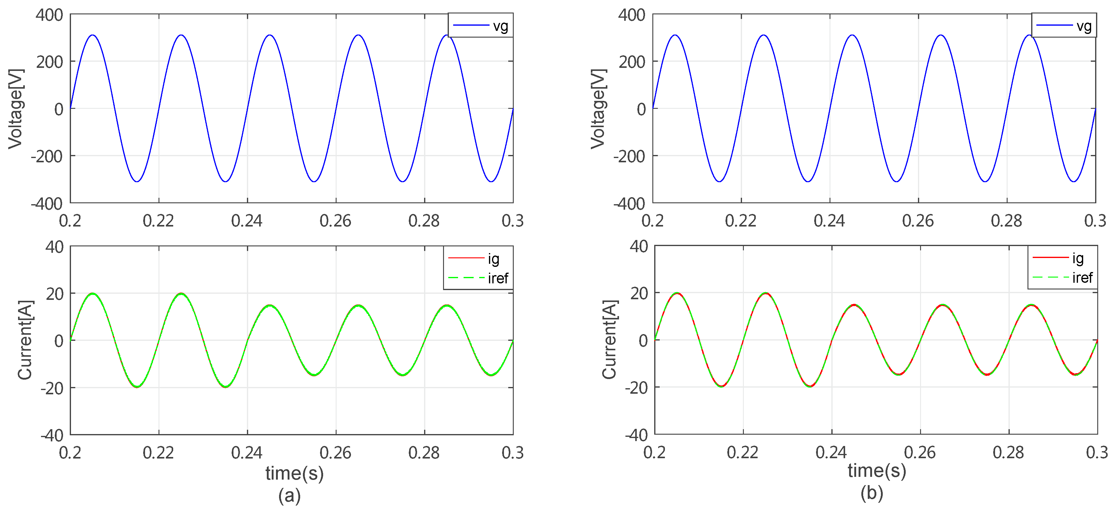
Due to the slow dynamic response of the traditional RC, a fast transient response should be achieved in the improved control scheme. When the given grid current reference steps from 20 A to 15 A at 0.24 s, the system dynamic response comparisons with the traditional PI control and the proposed PMQR-type repetitive control were as illustrated in Figure 23. It can be seen that the dynamic performance of the PMQR-type RC was almost the same as the PI control scheme. Just as mentioned in Section 3.3, fast dynamic response of the proportional controller will not be affected by slow RC, which indicates that the dynamic performance was mainly determined by the proportional controller, and the RC just like the MQR controller was only used to improve steady-state harmonics compensation.
5. Conclusions
In this paper, a PMQR-type repetitive current controller was designed for single-phase grid-tied H6-type inverters with an SOGI-based PLL. The proposed control scheme consisted of a repetitive controller and a proportional controller in parallel. The parallel structure can not only significantly reduce the design difficulty and cost compared with a PMQR controller, but also improve the capability of suppressing harmonics and the robust performance against grid disturbances. A detailed system modelling process and SOGI-based PLL design principles were introduced. A thorough stability analysis was also conducted, and the design steps of the proposed controller were given. The simulation results under different control schemes were compared, to verify the feasibility and superiority of the proposed controller.
Author Contributions
X.Y. designed the whole method for research. P.L. wrote the draft and the experiment. S.X. gave a detailed revision. S.L. provided important guidance for this paper. All authors have read and approved the final manuscript.
Funding
This work was supported in part by the National Science Foundation of China (51765042, 61463031, 61662044, 61862044), Jiangxi Provincial Department of Science and Technology JXYJG-2017-02.
Conflicts of Interest
The authors declare no conflict of interest.
References
- Adefarati, T.; Bansal, R. Integration of renewable distributed generators into the distribution system: A review. IET Renew. Power Gener. 2016, 10, 873–884. [Google Scholar] [CrossRef]
- Chen, D.; Zhang, J.; Qian, Z. An improved repetitive control scheme for grid-connected inverter with frequency-adaptive capability. IEEE Trans. Ind. Electron. 2013, 60, 814–823. [Google Scholar] [CrossRef]
- Dannehl, J.; Wessels, C.; Fuchs, F. Limitations of voltage-oriented pi current control of grid-connected pwm rectifiers with lcl filters. IEEE Trans. Ind. Electron. 2009, 56, 380–388. [Google Scholar] [CrossRef]
- Teodorescu, R.; Blaabjerg, F.; Liserre, M.; Loh, P.C. Proportional-resonant controllers and filters for grid-connected voltage-source converters. IEE Proc.-Electr. Power Appl. 2006, 153, 750–762. [Google Scholar] [CrossRef]
- Rashed, M.; Klumpner, C.; Asher, G. Repetitive and resonant control for a single-phase grid-connected hybrid cascaded multilevel converter. IEEE Trans. Power Electron. 2013, 28, 2224–2234. [Google Scholar] [CrossRef]
- Lopez, O.; Teodorescu, R.; Freijedo, F.; DovalGandoy, J. Leakage current evaluation of a singlephase transformerless pv inverter connected to the grid. In Proceedings of the APEC 2007-Twenty Second Annual IEEE Applied Power Electronics Conference, Anaheim, CA, USA, 25 February–1 March 2007; pp. 907–912. [Google Scholar]
- Ahmad, Z.; Singh, S. Single phase transformerless inverter topology with reduced leakage current for grid connected photovoltaic system. Electr. Power Syst. Res. 2018, 154, 193–203. [Google Scholar] [CrossRef]
- Islam, M.; Mekhilef, S.; Hasan, M. Single phase transformerless inverter topologies for grid-tied photovoltaic system: A review. Renew. Sustain. Energy Rev. 2015, 45, 69–86. [Google Scholar] [CrossRef]
- Yu, W.; Lai, J.-S.; Qian, H.; Hutchens, C. High-efficiency mosfet inverter with h6-type configuration for photovoltaic nonisolated ac-module applications. IEEE Trans. Power Electron. 2011, 26, 1253–1260. [Google Scholar] [CrossRef]
- Zhang, L.; Sun, K.; Xing, Y.; Xing, M. H6 transformerless full-bridge pv grid-tied inverters. IEEE Trans. Power Electron. 2014, 29, 1229–1238. [Google Scholar] [CrossRef]
- Panda, A.; Pathak, M.; Srivastava, S. A single phase photovoltaic inverter control for grid connected system. Sadhana 2016, 41, 15–30. [Google Scholar] [CrossRef]
- Chatterjee, A.; Mohanty, K. Current control strategies for single phase grid integrated inverters for photovoltaic applications—A review. Renew. Sustain. Energy Rev. 2018, 92, 554–569. [Google Scholar] [CrossRef]
- Hassaine, L.; Lias, E.; Quintero, J.; Salas, V. Overview of power inverter topologies and control structures for grid connected photovoltaic systems. Renew. Sustain. Energy Rev. 2014, 30, 796–807. [Google Scholar] [CrossRef]
- Yang, S.; Lei, Q.; Peng, F.; Qian, Z. A robust control scheme for grid-connected voltage-source inverters. IEEE Trans. Ind. Electron. 2011, 58, 202–212. [Google Scholar] [CrossRef]
- Sun, Z.; Wang, D.; Yuan, T.; Liu, Z.; Yu, J. A novel control strategy for grid-connected inverter based on iterative calculation of structural parameters. Energies 2018, 11, 3306. [Google Scholar] [CrossRef]
- Liserre, M.; Teodorescu, R.; Blaabjerg, F. Multiple harmonics control for three-phase grid converter systems with the use of pi-res current controller in a rotating frame. IEEE Trans. Power Electron. 2006, 21, 836–841. [Google Scholar] [CrossRef]
- Schiesser, M.; Wasterlain, S.; Marchesoni, M.; Carpita, M. A simplified design strategy for multi-resonant current control of a grid-connected voltage source inverter with an lcl filter. Energies 2018, 11, 609. [Google Scholar] [CrossRef]
- Yepes, A.G.; Freijedo, F.D.; López, O.; Doval-Gandoy, J. High-performance digital resonant controllers implemented with two integrators. IEEE Trans. Power Electron. 2011, 26, 563–576. [Google Scholar] [CrossRef]
- Pan, Z.; Dong, F.; Zhao, J.; Wang, L.; Wang, H.; Feng, Y. Combined resonant controller and two-degree-of-freedom pid controller for pmslm current harmonics suppression. IEEE Trans. Ind. Electron. 2018, 65, 7558–7568. [Google Scholar] [CrossRef]
- Zhao, Q.; Ye, Y. A pimr-type repetitive control for a grid-tied inverter: Structure, analysis, and design. IEEE Trans. Power Electron. 2018, 33, 2730–2739. [Google Scholar] [CrossRef]
- Trinh, Q.N.; Wang, P.; Tang, Y.; Choo, F.H. Mitigation of dc and harmonic currents generated by voltage measurement errors and grid voltage distortions in transformerless grid-connected inverters. IEEE Trans. Energy Convers. 2018, 33, 801–813. [Google Scholar] [CrossRef]
- Gao, Y.-G.; Jiang, F.-Y.; Song, J.-C.; Zheng, L.-J.; Tian, F.-Y.; Geng, P.-L. A novel dual closed-loop control scheme based on repetitive control for grid-connected inverters with an lcl filter. ISA Trans. 2018, 74, 194–208. [Google Scholar] [CrossRef]
- De, D.; Ramanarayanan, V. A proportional + multiresonant controller for three-phase four-wire high-frequency link inverter. IEEE Trans. Power Electron. 2010, 4, 899–906. [Google Scholar] [CrossRef]
- Gradshteyn, I.S.; Ryzhik, I.M. Table of Integrals, Series, and Products; Academic Press: New York, NY, USA, 2014. [Google Scholar]
- He, L.; Zhang, K.; Xiong, J.; Fan, S. A repetitive control scheme for harmonic suppression of circulating current in modular multilevel converters. IEEE Trans. Power Electron. 2014, 30, 471–481. [Google Scholar] [CrossRef]
- Zhang, B.; Wang, D.; Zhou, K.; Wang, Y. Linear phase lead compensation repetitive control of a cvcf pwm inverter. IEEE Trans. Ind. Electron. 2008, 55, 1595–1602. [Google Scholar] [CrossRef]
- Han, Y.; Luo, M.; Zhao, X.; Guerrero, J.M.; Xu, L. Comparative performance evaluation of orthogonal-signal-generators-based single-phase pll algorithms—A survey. IEEE Trans. Power Electron. 2016, 31, 3932–3944. [Google Scholar] [CrossRef]
- Özdemir, A.; Yazici, I.; Vural, C. Fast and robust software-based digital phase-locked loop for power electronics applications. IET Gener. Trans. Distrib. 2013, 7, 1435–1441. [Google Scholar] [CrossRef]
- Golestan, S.; Guerrero, J.M.; Vasquez, J.C. A nonadaptive window-based pll for single-phase applications. IEEE Trans. Power Electron. 2018, 33, 24–31. [Google Scholar] [CrossRef]
- Golestan, S.; Guerrero, J.M.; Vidal, A.; Yepes, A.G.; Doval-Gandoy, J.; Freijedo, F.D. Small-signal modeling, stability analysis and design optimization of single-phase delay-based plls. IEEE Trans. Power Electron. 2016, 31, 3517–3527. [Google Scholar] [CrossRef]
- Jiang, Y.; Li, Y.; Tian, Y.; Wang, L. Phase-locked loop research of grid-connected inverter based on impedance analysis. Energies 2018, 11, 3077. [Google Scholar] [CrossRef]
- Golestan, S.; Monfared, M.; Freijedo, F.D.; Guerrero, J.M. Dynamics assessment of advanced single-phase pll structures. IEEE Trans. Ind. Electron. 2013, 60, 2167–2177. [Google Scholar] [CrossRef]
Figure 1.
The overall control block diagram of a single-phase grid-connected H6 inverter. SOGI, second-order generalized integrator.
Figure 1.
The overall control block diagram of a single-phase grid-connected H6 inverter. SOGI, second-order generalized integrator.
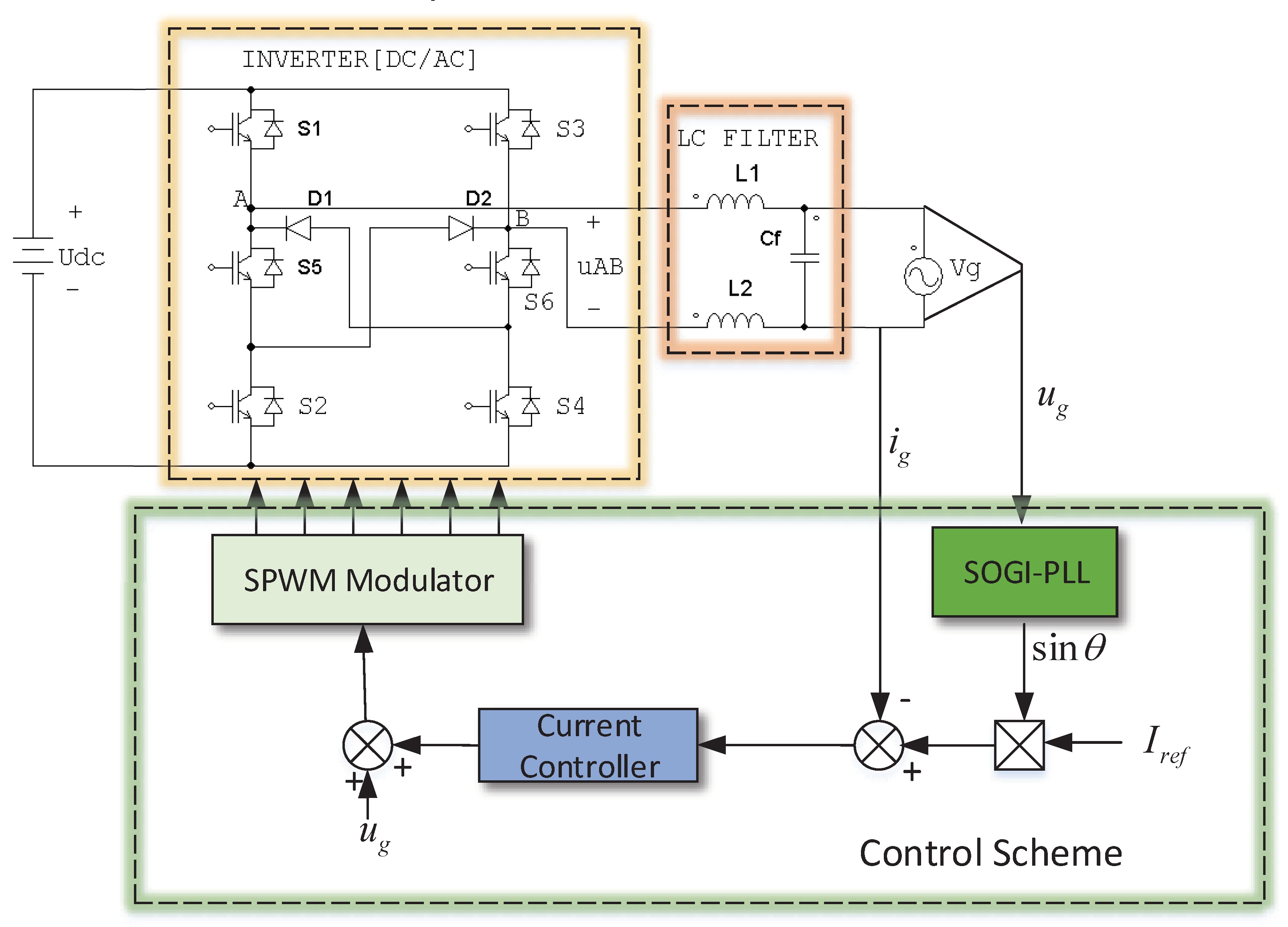
Figure 2.
The proportional multiple quasi-resonant (PMQR) controller for fundamental and harmonic components.
Figure 2.
The proportional multiple quasi-resonant (PMQR) controller for fundamental and harmonic components.

Figure 3.
The control structure of the PMQR-type repetitive control (RC) scheme.
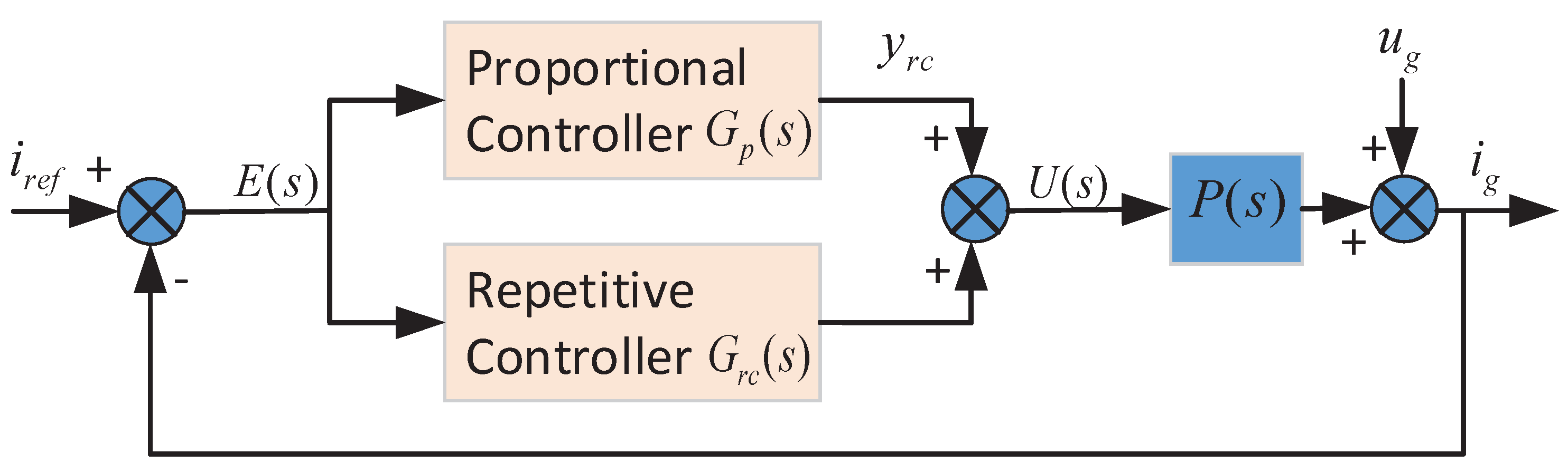
Figure 4.
The equivalent block diagram of .

Figure 5.
The detailed block diagram of the PMQR-type RC scheme.
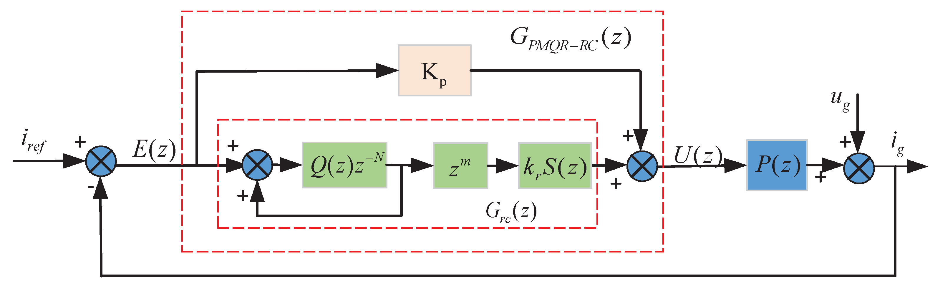
Figure 6.
Block diagram of the SOGI-PLL.

Figure 7.
Structure block diagram of SOGI-based OSG.
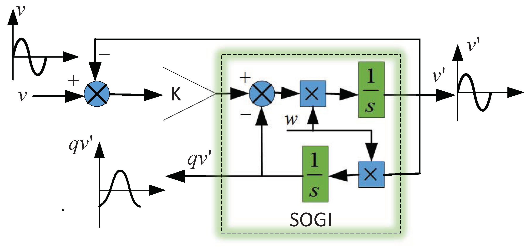
Figure 8.
Bode plot of the transfer function with different k.
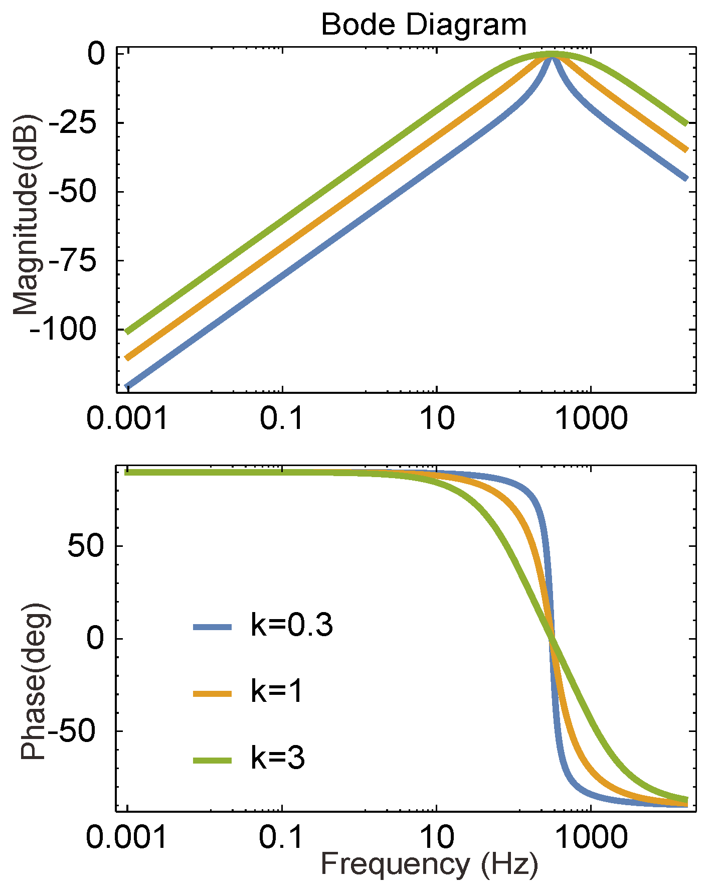
Figure 9.
The dominant pole assignment map of under different .
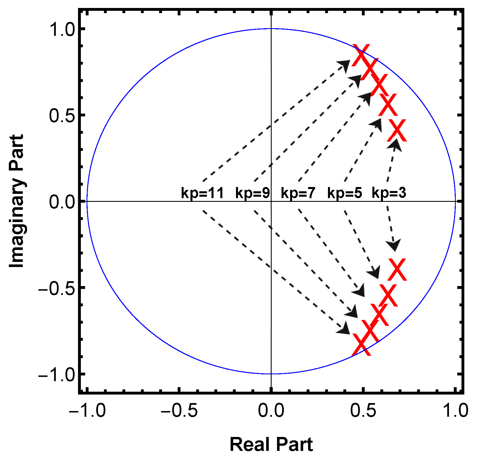
Figure 10.
Bode plot of under different .
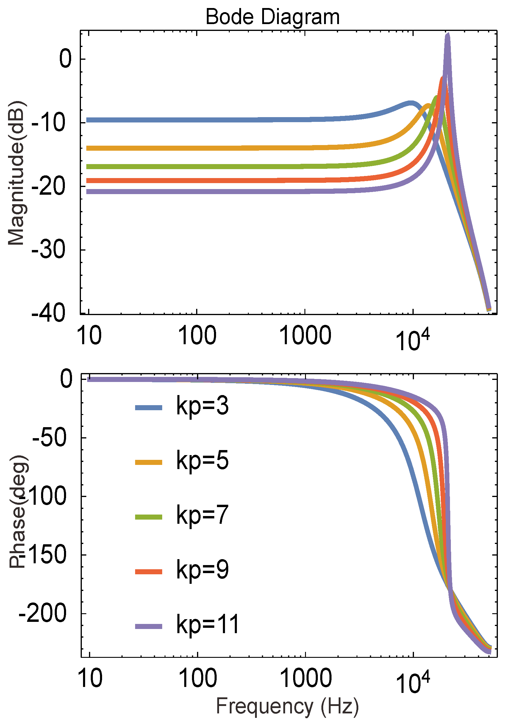
Figure 11.
Bode plot of the internal model of RC with different .

Figure 12.
Bode plot of the system after magnitude compensation.
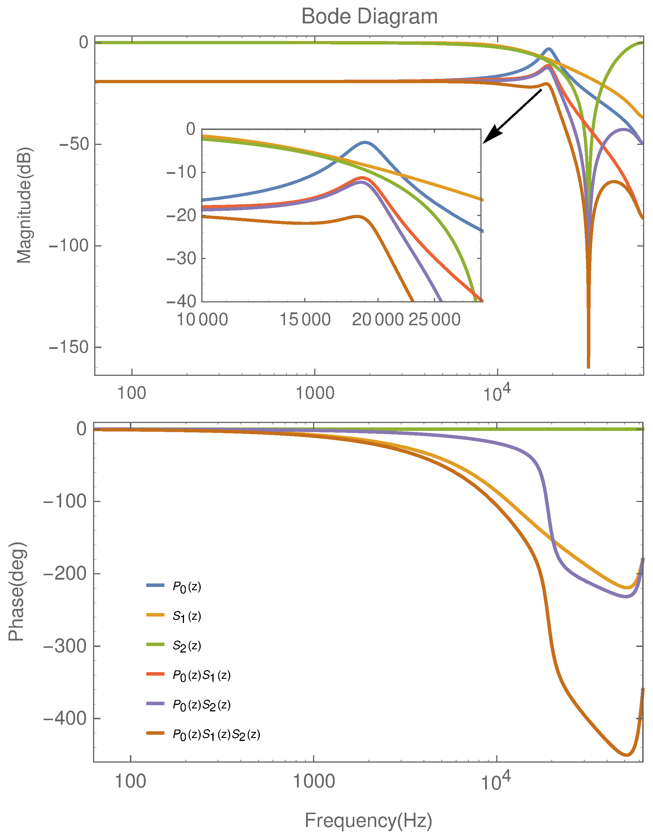
Figure 13.
Frequency characteristic of the system in different lead-links .
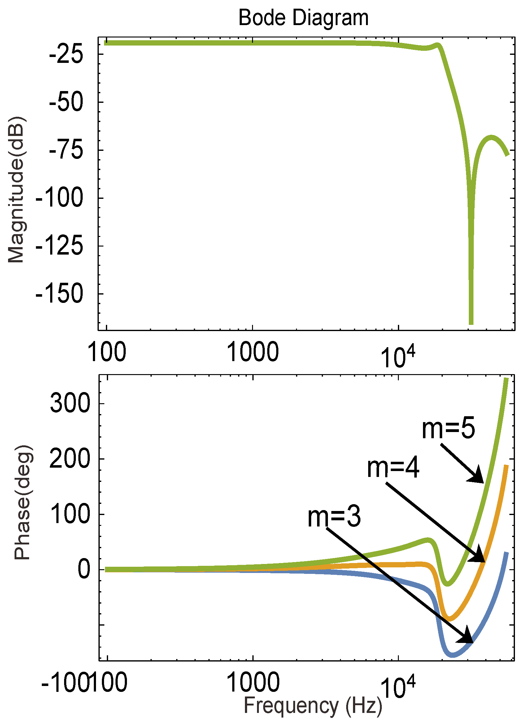
Figure 14.
Nyquist plot of with different values of .
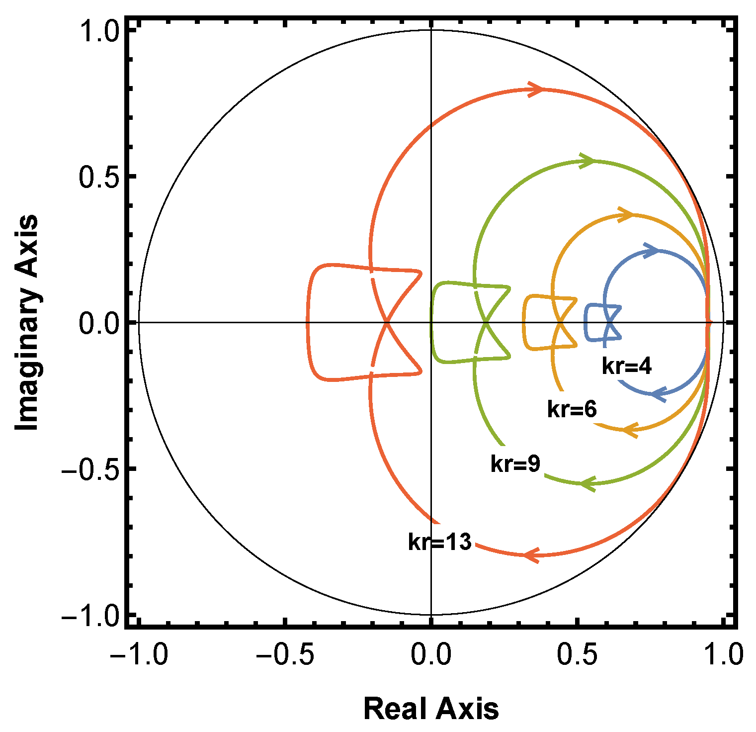
Figure 15.
The open-loop control gains of the PQMR-type RC and general RC .
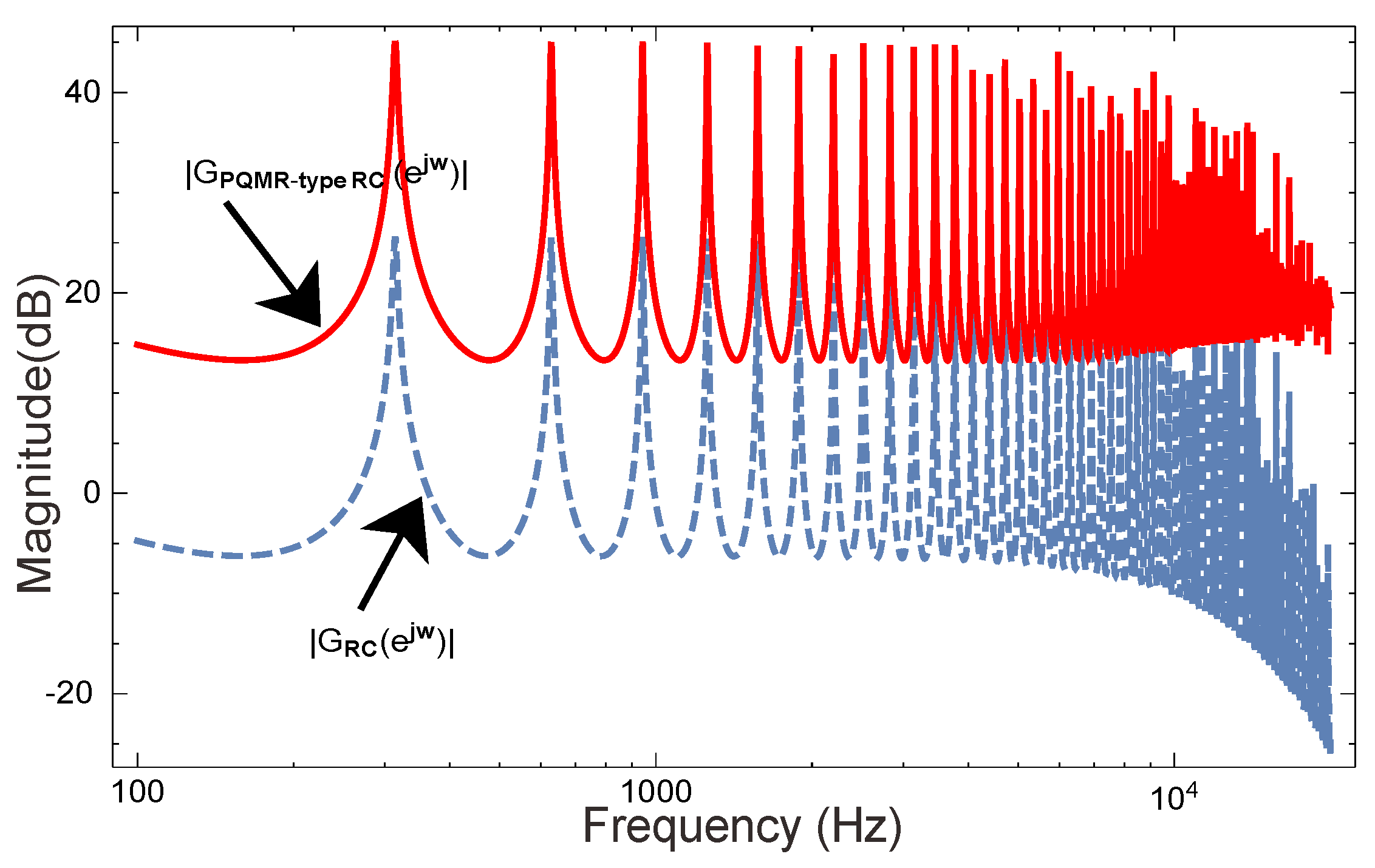
Figure 16.
The open-loop gains of , and general RC .
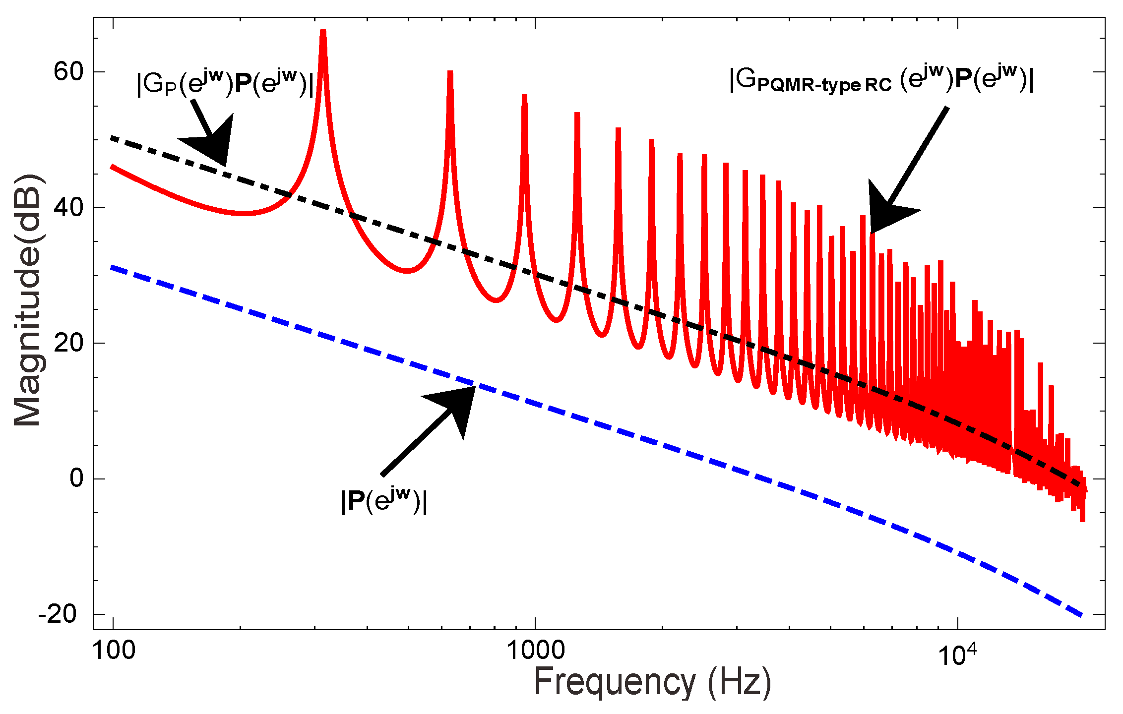
Figure 17.
Steady-state grid voltage and output current waveforms under different controllers. (a) With PI controller. (b) With PR controller. (c) With repetitive controller. (d) With PMQR-type RC controller.
Figure 17.
Steady-state grid voltage and output current waveforms under different controllers. (a) With PI controller. (b) With PR controller. (c) With repetitive controller. (d) With PMQR-type RC controller.
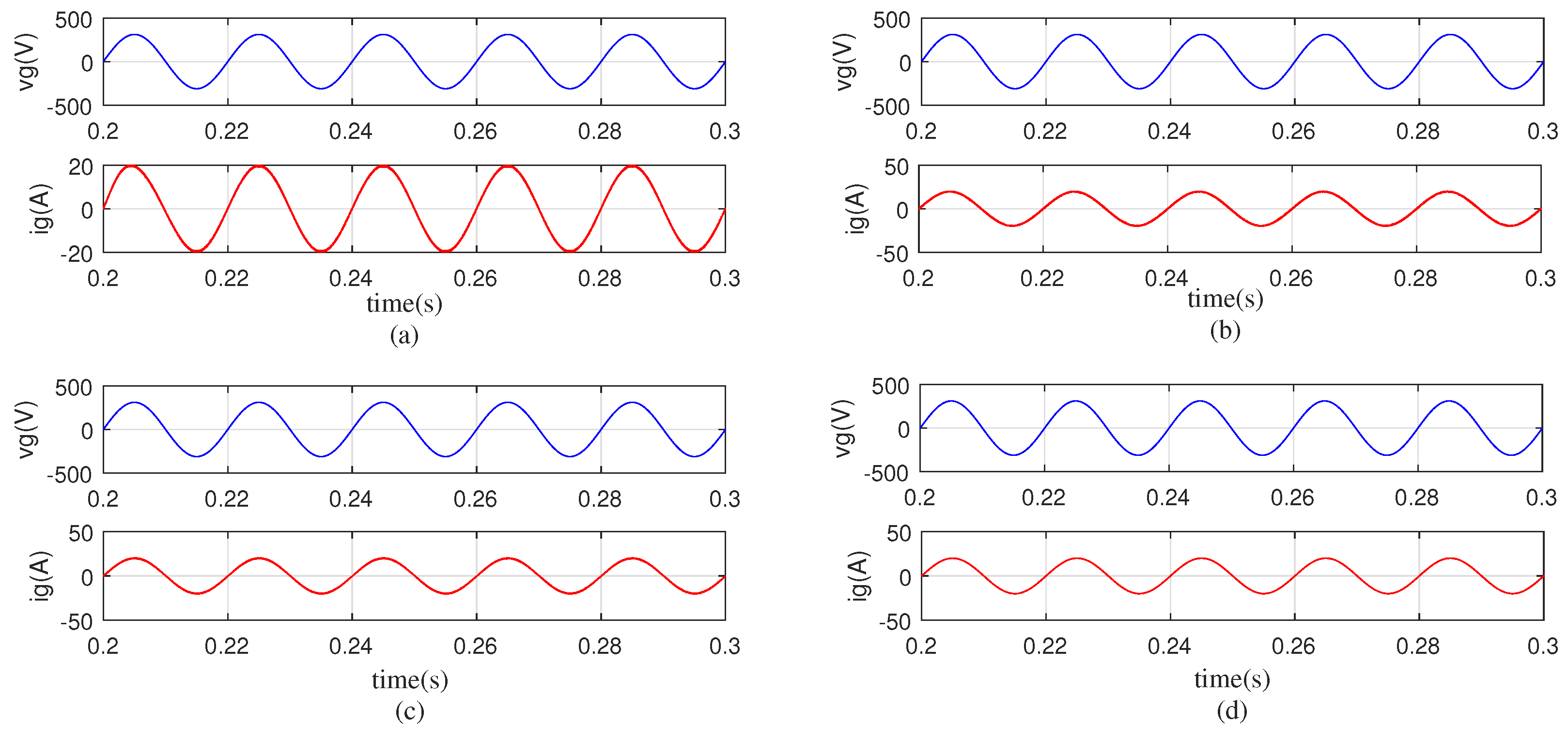
Figure 18.
The current tracking error in the steady-state with different controllers. (a) With PI controller. (b) With PR controller. (c) With repetitive controller. (d) With PMQR-type RC controller.
Figure 18.
The current tracking error in the steady-state with different controllers. (a) With PI controller. (b) With PR controller. (c) With repetitive controller. (d) With PMQR-type RC controller.

Figure 19.
FFT analysis plots of output current with different controllers. (a) With PI controller. (b) With PR controller. (c) With repetitive controller. (d) With the PMQR-type RC controller.
Figure 19.
FFT analysis plots of output current with different controllers. (a) With PI controller. (b) With PR controller. (c) With repetitive controller. (d) With the PMQR-type RC controller.
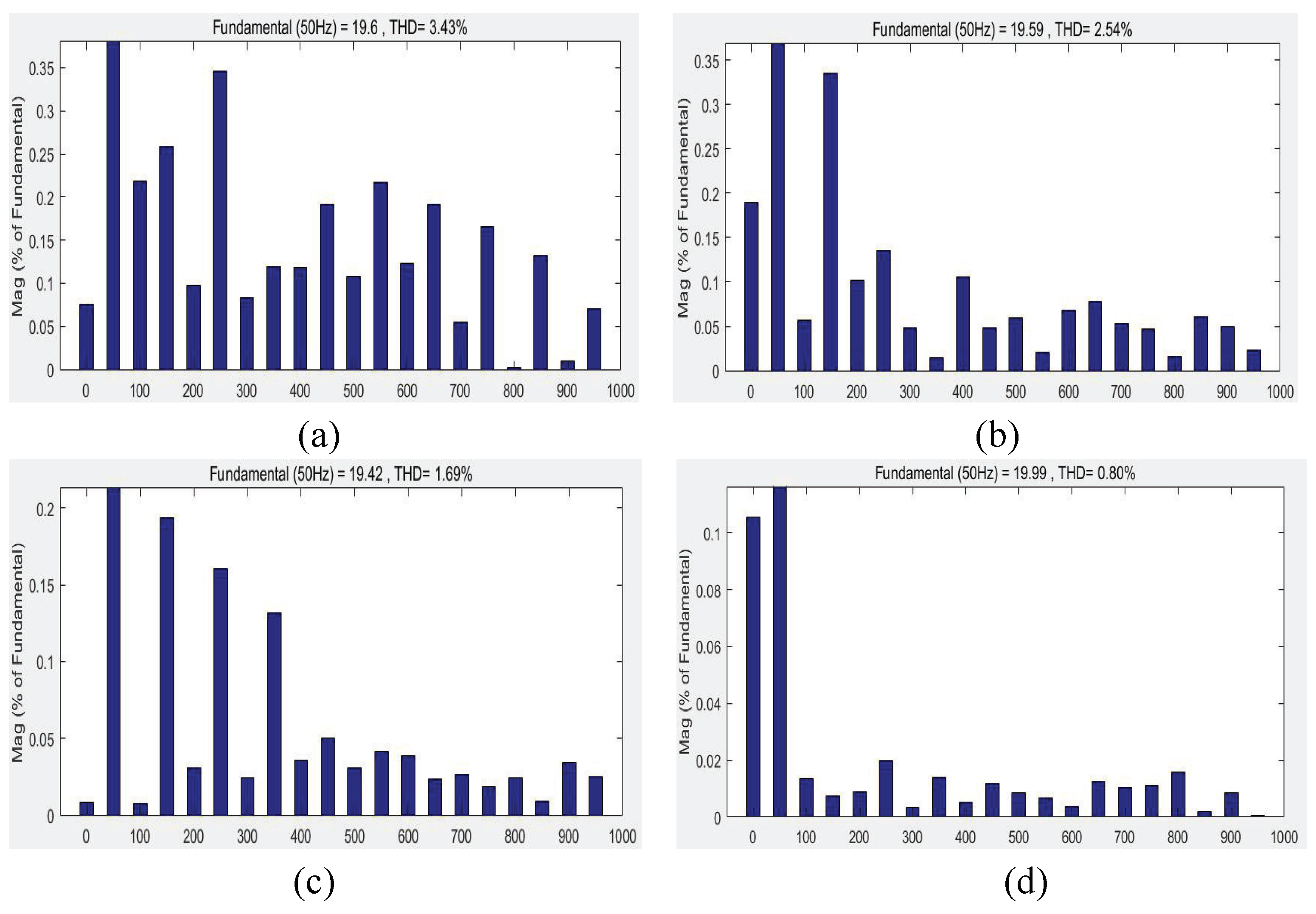
Figure 20.
Total harmonic distortion (THD) magnitude with current controllers.
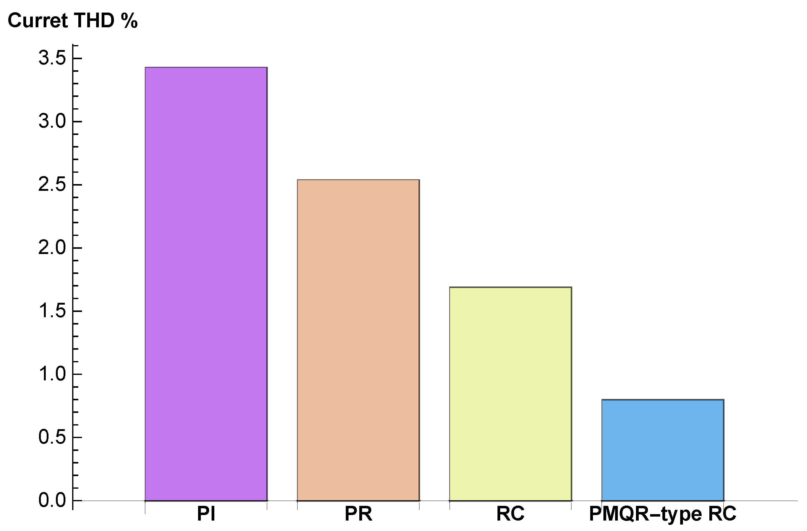
Figure 21.
Most prominent harmonic components of output current.
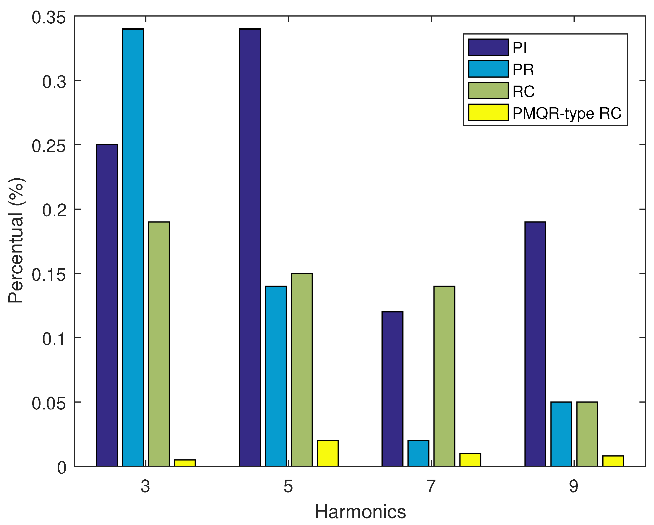
Figure 22.
THD magnitude of current controller during variation in frequency.
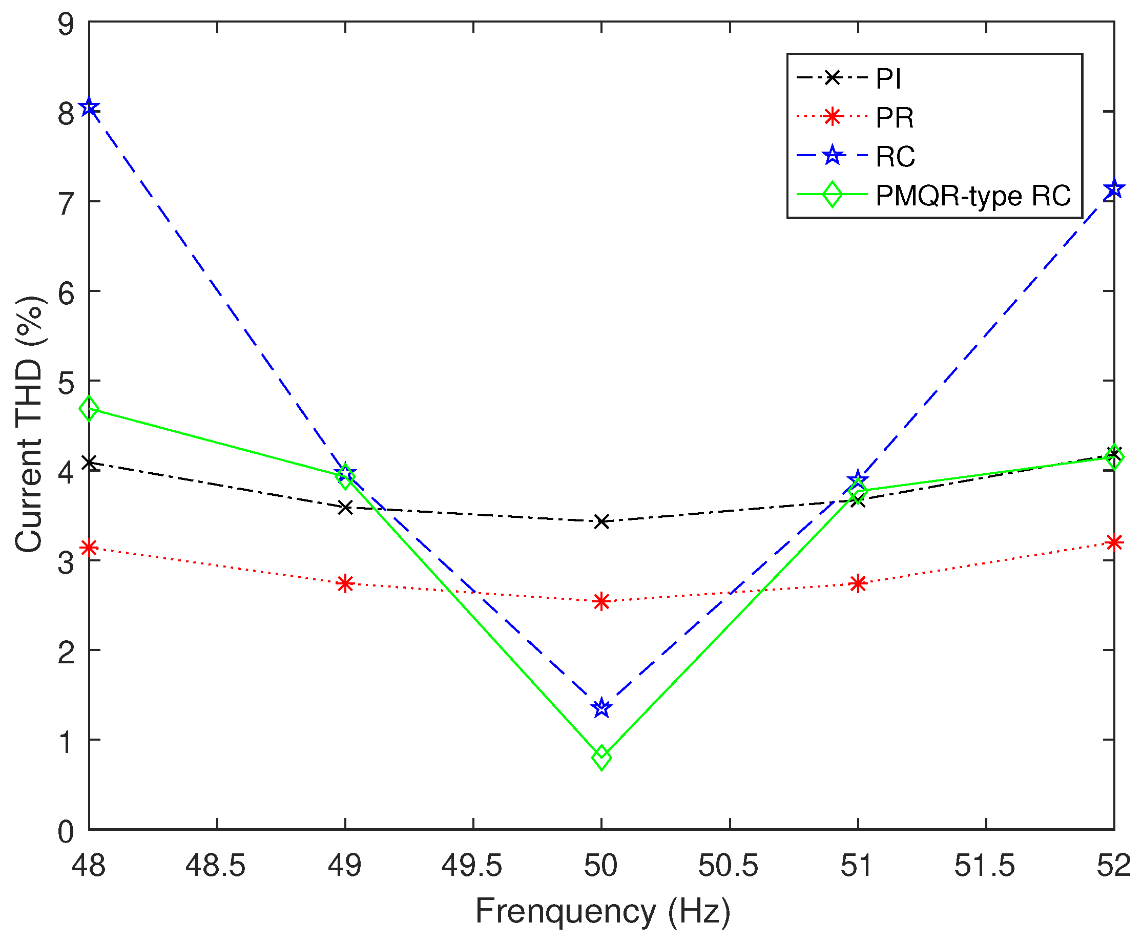
Figure 23.
The system dynamic response. (a) With PI controller. (b) With PMQR-type RC controller.

Table 1.
Parameters of the grid-connected H6 inverter with the LC filter.
| Symbol | Description | Values |
|---|---|---|
| grid voltage | 220 V | |
| ideal grid voltage frequency | 50 Hz | |
| DC bus voltage | 360 V | |
| sampling frequency | 20 kHz | |
| filter inductor | mH | |
| filter capacitor | 4 F | |
| R | ESR | 0.1 |
| P | output power | 3 kW |
© 2019 by the authors. Licensee MDPI, Basel, Switzerland. This article is an open access article distributed under the terms and conditions of the Creative Commons Attribution (CC BY) license (http://creativecommons.org/licenses/by/4.0/).
Share and Cite
MDPI and ACS Style
Yang, X.; Liu, P.; Xu, S.; Liu, S. Analysis and Design of A PMQR-Type Repetitive Control Scheme for Grid-Connected H6 Inverters. Appl. Sci. 2019, 9, 1198. https://doi.org/10.3390/app9061198
AMA Style
Yang X, Liu P, Xu S, Liu S. Analysis and Design of A PMQR-Type Repetitive Control Scheme for Grid-Connected H6 Inverters. Applied Sciences. 2019; 9(6):1198. https://doi.org/10.3390/app9061198
Chicago/Turabian StyleYang, Xiaohui, Peiyun Liu, Shaoping Xu, and Shichao Liu. 2019. "Analysis and Design of A PMQR-Type Repetitive Control Scheme for Grid-Connected H6 Inverters" Applied Sciences 9, no. 6: 1198. https://doi.org/10.3390/app9061198
Note that from the first issue of 2016, this journal uses article numbers instead of page numbers. See further details here.