Skin Aging Estimation Scheme Based on Lifestyle and Dermoscopy Image Analysis


1
School of Electrical Engineering, Korea University, 145 Anam-ro, Seongbuk-gu, Seoul 02841, Korea
2
Kiturami Research Planning Center, Co., Ltd., 40, Baekbeom-ro, 603 beon-gil, Seo-gu, Incheon 22830, Korea
*
Author to whom correspondence should be addressed.
Appl. Sci. 2019, 9(6), 1228; https://doi.org/10.3390/app9061228
Submission received: 14 February 2019
/
Revised: 21 March 2019
/
Accepted: 21 March 2019
/
Published: 23 March 2019
(This article belongs to the Special Issue Data Analytics in Smart Healthcare)
Abstract
:Besides genetic characteristics, people also undergo a process of skin aging under the influence of diverse factors such as sun exposure, food intake, sleeping patterns, and drinking habits, which are closely related to their personal lifestyle. So far, many studies have been conducted to analyze skin conditions quantitatively. However, to describe the current skin condition or predict future skin aging effectively, we need to understand the correlation between skin aging and lifestyle. In this study, we first demonstrate how to trace people’s skin condition accurately using scale-invariant feature transform and the color histogram intersection method. Then, we show how to estimate skin texture aging depending on the lifestyle by considering various features from face, neck, and hand dermoscopy images. Lastly, we describe how to predict future skin conditions in terms of skin texture features. Based on the Pearson correlation, we describe the correlation between skin aging and lifestyle, and estimate skin aging according to lifestyle using the polynomial regression and support vector regression models. We evaluate the performance of our proposed scheme through various experiments.
1. Introduction
Skin aging is a biological mechanism affected by various combinations of intrinsic and extrinsic aging factors. While intrinsic aging factors are represented by genetic characteristics and changes of hormones, extrinsic aging factors are represented by personal lifestyle and environmental factors, e.g., chronic sunlight exposure, cigarette smoking, air pollution. These factors, together, lead to cumulative structural and physiological alterations, and gradual changes in each skin layer as well as in skin appearance. Aside from genetic and natural factors, lifestyle is the most influential factor that affects skin condition. In dermatology, abrupt skin deterioration is considered to be deeply related to everyday activities such as excessive eating, drinking, sunlight exposure and lack of sleeping.
To investigate the correlation between skin aging and lifestyle, we need to continuously monitor any changes in the skin condition and its cause. Using this correlation, we can eventually predict the future of the skin condition according to the lifestyle. To do this efficiently, in this paper, we propose a scheme for tracing the correlation between the skin condition and lifestyle and estimating skin aging based on the correlation.
In general, dermatologists look into the shape of skin texture to diagnose the condition of the skin, the most significant ones of which include the width, length, and depth of wrinkles. So far, many studies have been done to objectively evaluate skin aging through skin texture image.
After 2000, most evaluations of skin surface used are captured by molding replicas to observe texture shape and surface topologies via 3D image modeling progress [1,2,3,4,5]. Yow et al. presented a skin analysis system that can identify and quantify skin characteristics such as the topography of skin surface and thickness automatically using 3D modeling processing [3]. Pirisinu and Mazzarello proposed a silicone replica analysis method for constructing 3D skin structure. They utilized the MEX Alicona software and scanning electron microscopy (SEM) to analyze skin topography quantitatively [4]. Replica-based analysis methods take a long time and are costly for diagnosis because they are involved with a complicated process and require expensive equipment.
Recently, 2D image analysis of skin texture methods [6,7,8,9,10,11] has tended to overcome these shortcomings. Tanaka et al. proposed various image processing methods for evaluating skin condition. They collected 50x magnified skin images and calculated the wrinkle thickness [6]. Hamer et al. described a new scheme for extracting skin texture to measure skin aging [7]. Zou et al. focused on the objective characterization of the skin surface and proposed a new parameter to represent the area mean of a skin texture block [8]. Trojahn et al. found the relationship between skin surface topography, roughness, and skin aging by investigating the number of closed polygons per measurement field [9]. Xie et al. proposed a skin texture pattern analysis scheme for personal identification and gender classification. They used the skin texture image of the back of the hand and various image filters for identifying texture characteristics [11].
Skin aging is a gradual process represented by the characteristic change in skin and one of the most obvious symptoms of human aging [12,13,14,15,16,17,18,19]. There have been many studies to clarify the relationship between progression of skin aging and skin texture change. For instance, Gao et al. proposed an image processing technique to calculate some of these skin texture parameters, focusing on the correlation of sun exposure history, demographic information and skin texture parameters [13]. Miyamoto et al. developed a quantitative method for analyzing facial skin elasticity rapidly and showed how skin elasticity is correlated to moisturization [14]. Haluza et al. investigated the effect of one-year prevalence of sun exposure and skin health-associated knowledge. They statistically analyzed that skin disease and aging can occur rapidly according to sun exposure time and personal life patterns [15]. Park et al. analyzed the effect of particulate matter (PM) on skin aging. They demonstrated that PM contributes to skin inflammation and skin aging [19].
Prediction of aging on the body organs has been considered a very challenging task because aging is complicated by various factors such as health, gender, and lifestyle. So far, many researchers have attempted to predict aging [20,21] by considering the life activity pattern [22,23]. For instance, Yang et al. proposed a facial aging simulation scheme that can simulate aging effects on the facial image. They applied the person-specific facial properties for facial aging simulation [20]. Suo et al. proposed a dynamic prediction model that predicts face aging using the Markov process and presented a compositional model that organized the face into parts such as hair and wrinkles [21].
To summarize, considerable research has been conducted on skin aging and aging estimation, but a major problem with understanding such relation between skin aging and lifestyle is a lack of practical methods and systems. To address this issue, we propose the following three primary contributions. 1) We present useful tracing methods for the region of the observation area, which combines scale invariant feature transform (SIFT) and the color histogram intersection methods. 2) We apply visual texture extraction methods that provide reasonable results for the skin condition and experimentally determine the correlation between skin condition changes and lifestyle data. To the best of our knowledge, if we know the cause of skin aging, it is possible to infer the skin condition that will be changed after a certain period. 3) We propose an aging simulation system based on the feature changes trends and obtain reasonable estimation results. We believe that it will be a useful tool for understanding the skin texture aging progress with lifestyle changes.
2. Methods
2.1. Our Previous Work
We previously proposed a skin texture extraction scheme for quantitative skin aging trend analysis [24,25,26]. We developed three major steps for skin texture analysis and tried to improve the visual feature quality [25]. Through this process, we verified that the visual skin aging trend is closely related to actual aging [26]. And then, to quantitatively calculate the effect of lifestyle on skin condition changes, we developed the matric called SDS (Skin Damaging Score) which formulated the influence of life activities on skin aging [27]. However, skin aging patterns can be different for each person. For example, depending on personal lifestyle, skin aging progress can appear quickly or slowly. In this study, we consider the personal characteristics affected by lifestyle.
2.2. Skin Texture Location Mapping
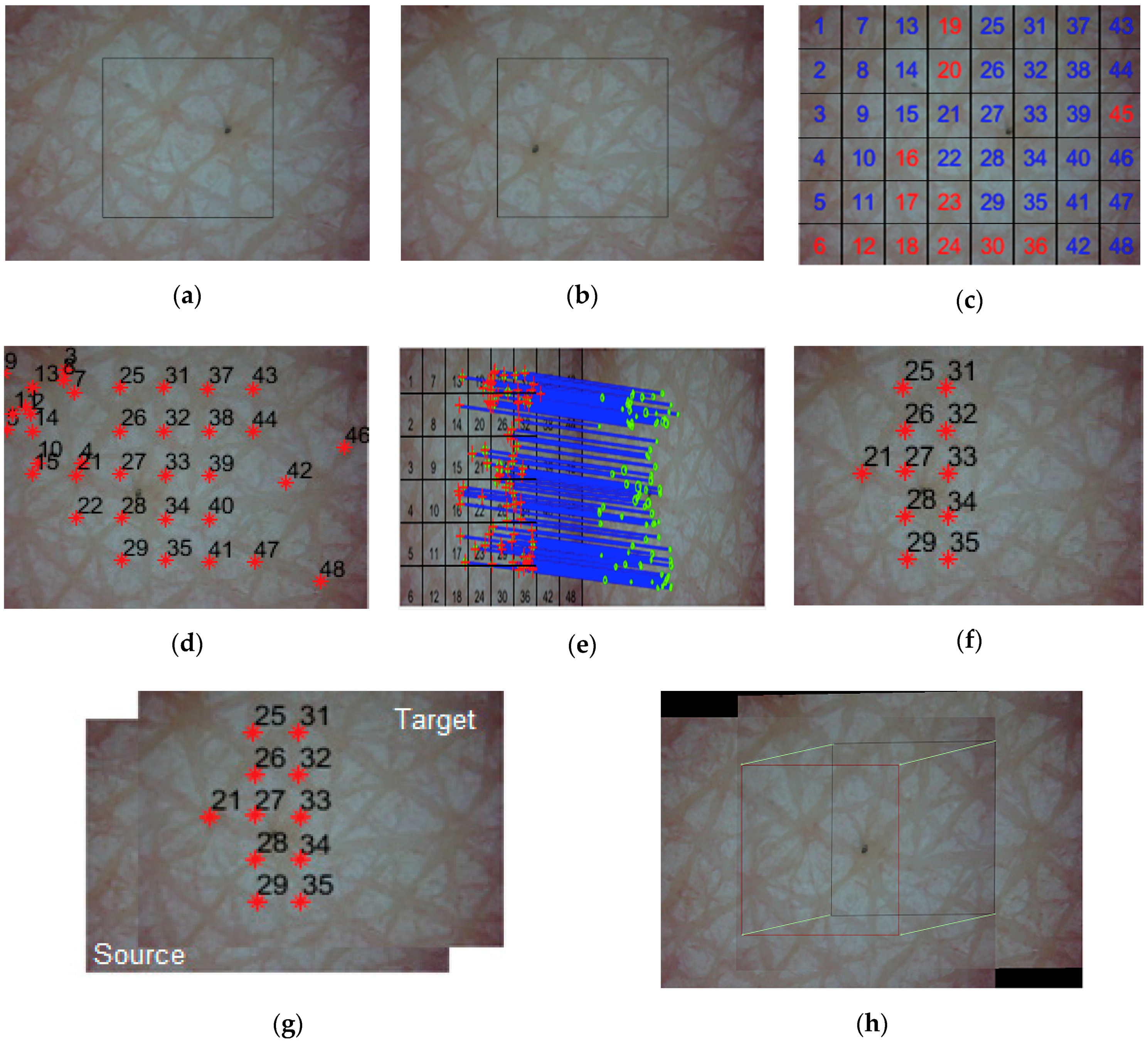
When tracing and observing the skin condition periodically, it is important to compare the same location of skin. However, due to camera device limitation and capturing wrong region of interest (ROI) location of skin, it is difficult to observe the skin condition precisely. Therefore, we applied the SIFT and color histogram mapping methods when periodically analyzing the skin texture images. SIFT [28] is a very popular algorithm in the image processing field for detecting and describing local features in images. However, SIFT does not consider the color information in the feature matching. Therefore, we performed the color histogram mapping before SIFT matching. For the color histogram intersection, we divided the source image into K grid regions. Then, we calculated the RGB color histograms on each grid region and performed normalized cross correlation (NCC) on the target image. Figure 1c shows the example of an image divided into 48 grids. Blue numbers on the grids indicate that NCC(k) ≥ 0.8 and the red numbers indicate that NCC(k) < 0.8. The numeric value of 0.8 was selected through extensive experiments for finding optimal geometric parameter. Following Equation (1), we calculate the NCC result for each grid K.
where k and n indicate the number of grids and the total number of pixels, respectively. Also, f and t indicate the sub-image of the source image and the target image, respectively. Using Equation (1), we can find similar regions between the sub-image and target image. Figure 1d shows the NCC matching results, which show highly correlated regions between the source and target images. Figure 1e shows the feature matching results using the SIFT algorithm. We calculated the number of matched feature points on the grids. If the matched SIFT feature points did not exist on the grids, we did not consider the grids for location mapping. Based on SIFT matching Figure 1e and NCC results Figure 1f, we calculated the same location between the source image and target image following Algorithm 1. Figure 1g,f show the overlapped and warped intersected grids between the source and target image using homographic computation [29].
| Algorithm 1. Warping region |
| Input: source image S, target image T Output: warped region of interest WROI |
| = () = () = (T) = false for each grid sg in for each grid tg in NCCindex = (sg, tg) matchedSIFT = ((sg, tg)) if (NCCindex 0.8 & matchedSIFT > 0) = true endif endfor endfor MatchPoints = () MatchPoints = () WarpPara W = ) WROI = (, W) return WROI |
2.3. Pre-Processing and Skin Feature Extraction
In this section, we briefly describe our skin feature extraction process. After texture location mapping, we first eliminated any excessive noise and vignetting effect induced by camera device limitations and light source interference. To analyze the skin texture accurately, we calculated skin features including wrinkle length, wrinkle width, wrinkle depth, wrinkle-bordered polygons and cell-related features [25,26,27] from the skeleton image, which is a one-pixel line skin texture generated from a dermoscopy image [25]. Also, from the skeleton image, we recovered the wrinkle width using a morphological region growing method. For the wrinkle depth, we defined the relative depth based on the color difference between the wrinkled and non-wrinkled regions. In addition, to identify wrinkle cells enclosed by the wrinkle border lines, we carried out the polygon mesh detection algorithm (PMDA) [26], which calculates the number of cells, cell area, and cell gradient. For instance, for the ROI and skin feature shown in Figure 2a,b, respectively, Figure 2c,d show recovered skin width and wrinkle cell gradients, respectively.
2.4. Skin Aging Estimation Model
Based on the diverse skin texture features, we first built a skin aging trend model using diverse regression techniques. We considered the polynomial regression and the support vector regression (SVR) for baseline analysis. Polynomial regression is very flexible and useful where a model must be developed empirically. In addition, it provides a good approximation and estimation of the relation between two independent variables. SVR is based on the computation of a linear regression function in a high-dimensional feature space where the input data are mapped via a nonlinear function. SVR has been very popular in the diverse fields such as sequential data prediction, approximation of complex engineering analysis, etc. To find the best polynomial regression, we propose Algorithm 2.
| Algorithm 2. Finding best polynomial regression model |
| Input: observed data S, time sequence T, n-th polynomial regression Output: optimized polynomial regression model OM |
| foreach degree n : = (S, T, n) : = ((), ()) if ( nbest: = endif endfor OM: = return OM |
Algorithm 2 describes curve fitting steps. For finding the best polynomial, we increased n and examine the goodness of fit by calculating the sum of squares error (SSE) and adjusting the R-square statistics. SSE indicates a better fit with a value closer to zero. The adjusted R-square statistic is generally the best indicator of the fit quality. For checking the accuracy of the curve fit, we used the confidence bounds on the coefficients. First, given a dataset with n independent variables and m observations, the regression model is generally expressed as , where and X are a vector of coefficients and a vector of independent variables, respectively, and b is the intercept. For selecting the best fitting model, we minimized the SSE.
For generating the estimation baseline, we used the SVM, which includes SVR for prediction and support vector classification (SVC) for classification. SVR differs from polynomial regression in the underlying theoretical settings. To avoid the prediction errors from outliers, we used the kernel functions and parameters to control the prediction errors. Equation (3) indicates how to construct the hyperplane to predict values.
Unlike Equation (2), the SVR method has two parameters: C and ε. Parameter C is introduced to adjust the error sensitivity of the training data in order to avoid over-fitting; setting C to a high value results in fewer prediction errors in the training data. Parameter ε is a regularization constant, which controls the flatness of the final model. To determine parameters, we carried out a grid search through a set of parameters, performing cross-validation. Then, we selected the optimal parameters with the best model performance.
In order to estimate skin aging associated with lifestyle, we assumed three types of lifestyle changes: 1) current lifestyle will be maintained in the future; 2) current lifestyle will be changed to accelerate the skin aging; and 3) current lifestyle will be changed to maintain the current skin condition. We called them ‘normal,’ ‘negative,’ and ‘positive,’ respectively. Based on this assumption, we defined two classes for skin aging status: ‘aging’ and ‘stopping’. The transient pattern of skin texture aging is affected by personal lifestyle. To classify the transient pattern, we considered the naïve Bayesian model which assumes that no relevance can be generated between different life activities.
In Equation (4), indicates the life activity value which is converted using SDS equations [27] from the observation period and indicates changes in skin status. indicates the type of life activities. In this study, we used five types of life activities. Using the following equation, we predicted skin status using life activity data.
2.5. Finding Relation between Skin Texture and Lifestyle
In real life, we frequently observe that skin conditions are affected by life activities. To find out their correlation, we needed to collect the activity data from subjects and analyze their effect on skin conditions. To investigate the correlation between activity pattern and skin aging, we collected user activity data from a smartphone and defined the activity type such as sleeping, basal metabolic rate (BMR), sun exposure, and drinking [27]. To determine the correlation coefficients, we performed the Pearson correlation coefficient test. The significance of the difference in each of the skin texture features among the life activities was analyzed through repeated measures of ANOVA for the paired data. We evaluated the relations among the wrinkle length, width, depth, cell-related features, and the activity features. The significance level was set at 0.05 and the confidence interval was set at 95%. A level of P < 0.05 was considered statistically significant.
2.6. Skin Aging Simulation
Based on the skin aging trend estimation results, we simulated the skin texture aging as shown in Figure 3. First, we extracted skin texture features from Section 2.3. Through the estimation models of each skin feature obtained through Section 2.4, we obtained the skin feature value at the desired age and set it as the simulation target value. After the target values were determined, we separated the wrinkle and cell regions to simulate the aging process.
Figure 4 shows an example of skin cell and wrinkle region clustering. For calculating the color histogram, we applied the K-means algorithm to the L*a*b* color regions of the two separated regions, respectively. We separated the color region using a K value of five and obtained the average and standard deviation of the L*a*b* color corresponding to each cluster. By subtracting the standard deviation value from the average that each cluster can have, we obtained the effect of image darkening. We repeatedly performed until the value of the prediction targets was reached.
Figure 5b,c show the translated cell color region and the translated wrinkle color regions, respectively. Figure 5d shows the result of merging the two images. After color translation for the wrinkle and cell regions was performed, we performed eight neighbors (left-top, top, right-top, left-middle, middle, right-middle, left-down, down and right-down) expansion based on the left and right skeleton of the wrinkle.
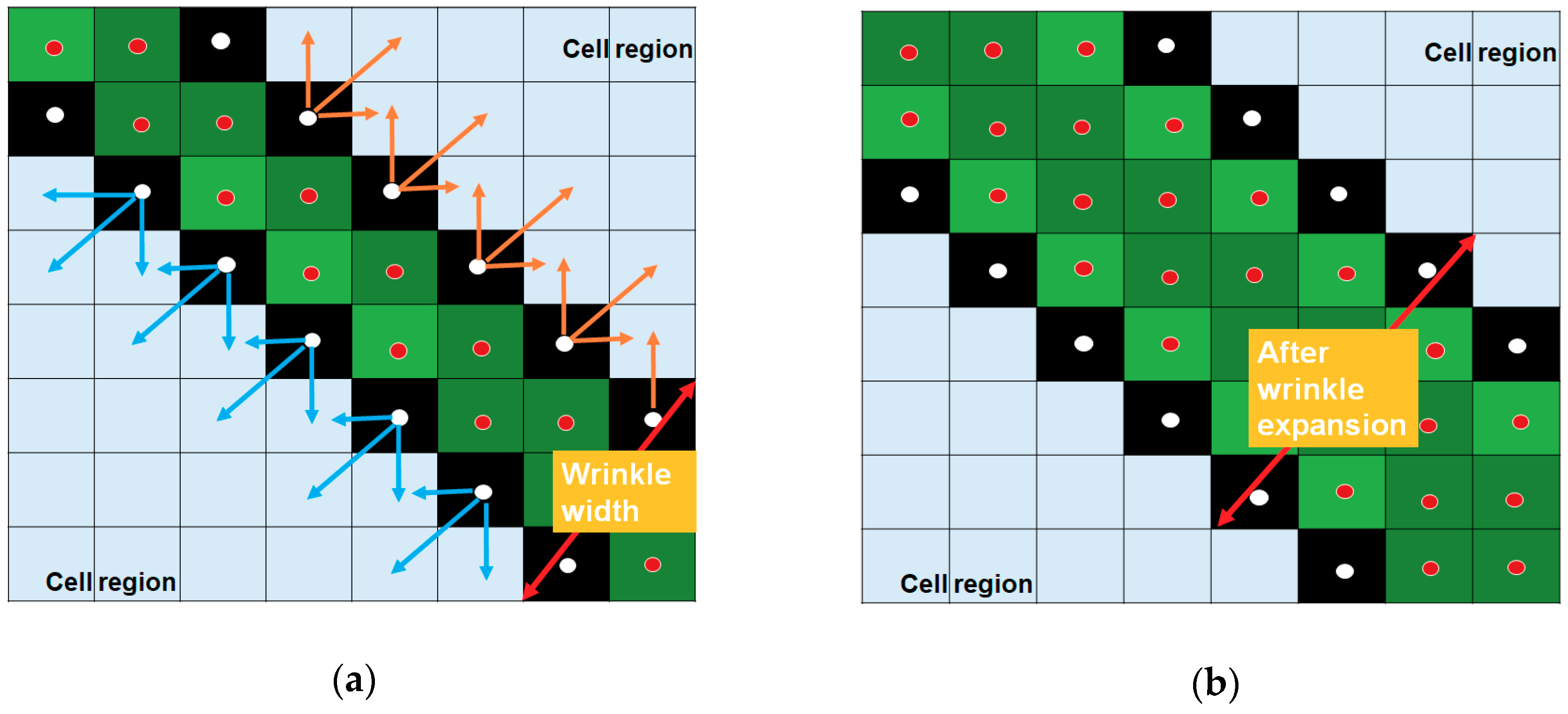
Figure 6a,b indicate the examples of wrinkle width expansion. Before expanding the wrinkle width, we checked the valid expansion points using the color histogram comparison. For eight-neighbor wrinkle width expansion, we proposed the wrinkle width expansion algorithm, which is based on clustered results. Algorithm 3 indicates how to expand the wrinkle width using clustered wrinkle regions. After wrinkle width expansion, we performed cell area and vector expansion.
Figure 7 provides a brief explanation of cell vector expansion. We calculated the cell vector using starting point A and ending point B. In Figure 7a, the black marked pixel indicates the wrinkle skeleton. The light blue, blue, and red pixels represent different cell regions. We define the maximum diameter of a cell region as a cell vector. In addition, the angle between the start point and end point is defined as θ. The cell vector increases with expansion weight EW and expansion angle α. We set the targets of cell vector length and angle from the estimation model of SVR and polynomial regression. Until reaching the target, we gradually increased EW and α. Algorithm 3 indicates the cell vector expansion process. First, we calculated the location of start point A and end point B from each cell region.
| Algorithm 3. Wrinkle width expansion |
| Input: wrinkle regions cluster , wrinkle skeleton Output: wrinkle width expanded image S |
| foreach wrinkle skeleton S(x,y) adjacent point(x,y) = (S(x,y)) for each wrinkle region clusters for each adjacent point (x,y), [] = ((x,y)) [] = (()) = indexmin = () (x,y) = S(x,y) = (x,y) endfor endfor endfor end return S |
Following Algorithm 4, we then calculated the cell vectors and expanded cell vectors. If the average of the cell vector length and angle reached the target value, the algorithm stops and overlaps all processed pixels on the image. Figure 8 shows the results of cell vector expansion. The red straight line in Figure 8c,d indicates the cell vectors that pass through the center of gravity of the cell. We performed the cell vector expansion iteratively until reaching the target cell vector’s length and angle.
| Algorithm 4. Cell vectors expansion |
| Input: cell regions , expansion weight EW, expansion angle , target cell vector length TCVL, target angle TA Output: Expanded cell regions |
| foreach cell regions startpoint (x,y) = () +[1 −1] * () * cos() endpoint () = () + [1 −1] * () * sin() cellvector = expandedcellvector = * cos() * EW endfor if (Avg(Length())) for each pixel (x,y) in cell regions = (x,y) * cos() * EW = () endfor else break return |
3. Result and Discussion
3.1. Study Population and Experiment Envoirnment
We used face, hand and neck 50X magnified dermoscopy images which were captured twice from the skin clinical research center in Korea. The skin research center selected 365 healthy subjects. They spent most of their time in indoor environments and maintained normal life patterns. The data collection period was from December 2013 to February 2014. Due to the cold weather, the subjects did little outside activities. The subjects’ skin types were classified as dry, complex, normal, and oily. To maintain a subject’s consistent skin condition, the dermatologist asked subjects to limit excessive exercising, drinking, outdoor activities and lack of sleeping time for several days. The dermoscopy images were carried out in a controlled space at a temperature of 23 ± 3 °C and relative humidity of 50 ± 10% with any cosmetics. The dataset was constructed in six classes, and sixty subjects belonged to one class. To analyze the correlation between changes of skin texture and life pattern, we selected the four subjects and observed their daily activities and skin texture images during the eight weeks. Four subjects completed a questionnaire including time duration of outdoor, physical activity, smoking history, drinking history, food intake, and sleeping time. To obtain the best condition of the skin texture image, we captured images from the four subjects around 2:30 pm, when skin form has the best coordination. Figure 9 shows the application interface of our system, which is developed in MATLAB 2016a version.
3.2. Skin Texture Location Mapping
For skin texture location mapping, we set the number of grids as 4, 48, and 108. For the experiments, we captured 132 skin texture images of the face and hand. Among them, 80 images contained the same regions to be analyzed and 52 images did not contain the same regions. Figure 10 shows examples of the experimental dataset. Figure 10a indicates the source image and Figure 10b,c indicate the matching target images, which has or does not have the warping region of the source image. If during the location mapping, the warping regions were found, the ROI existed in the target image. On the contrary, the warping regions were not found and the ROI did not exist in the target image. For evaluating the accuracy of texture location mapping, we set Equation (5) and calculated the accuracy of ROI warping. ROI calculates a size of 300 × 300 around the image center. If warping regions were not found, we classified it as a different image.
3.3. Trend Analysis of Skin Texture Aging
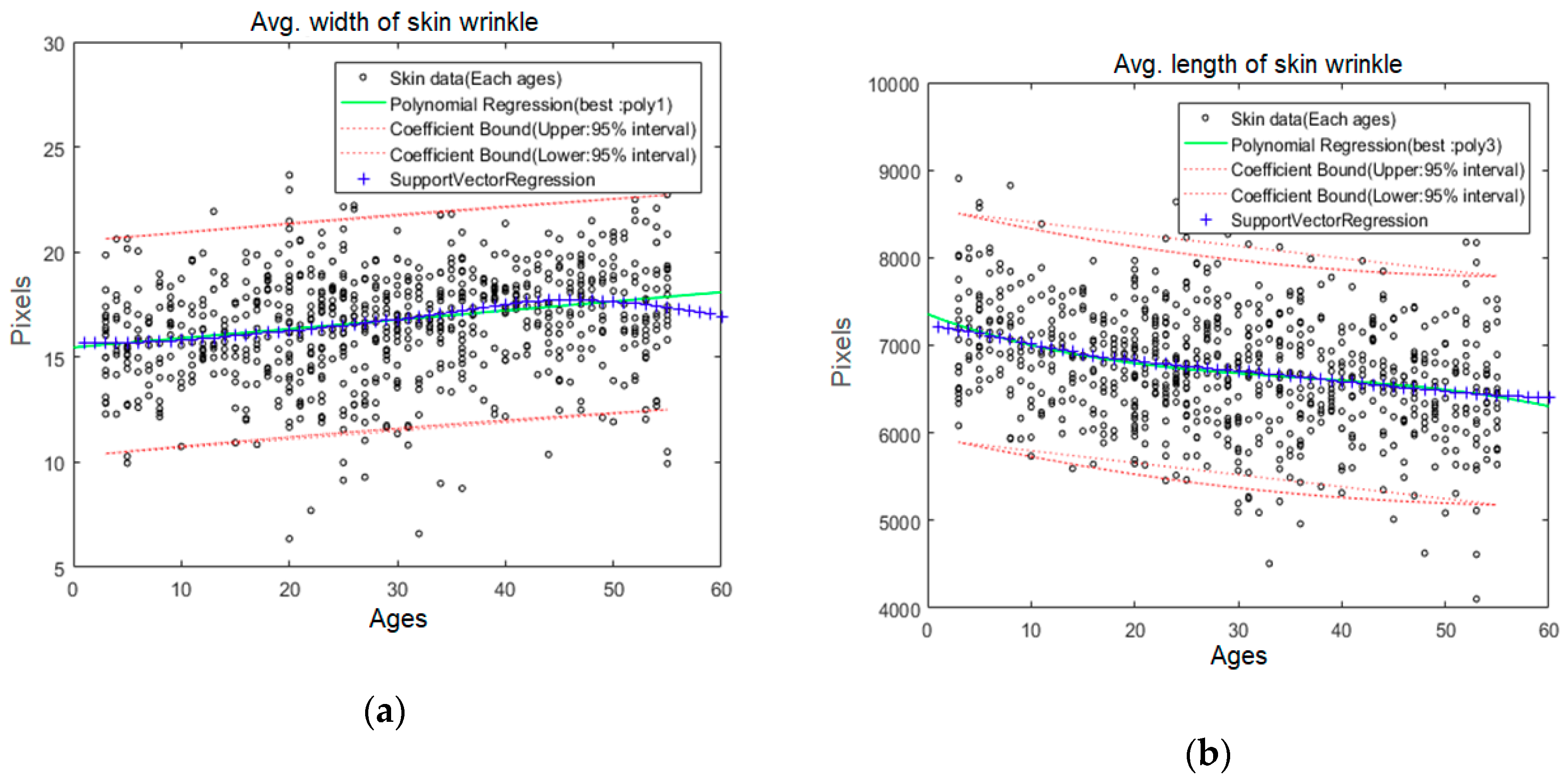
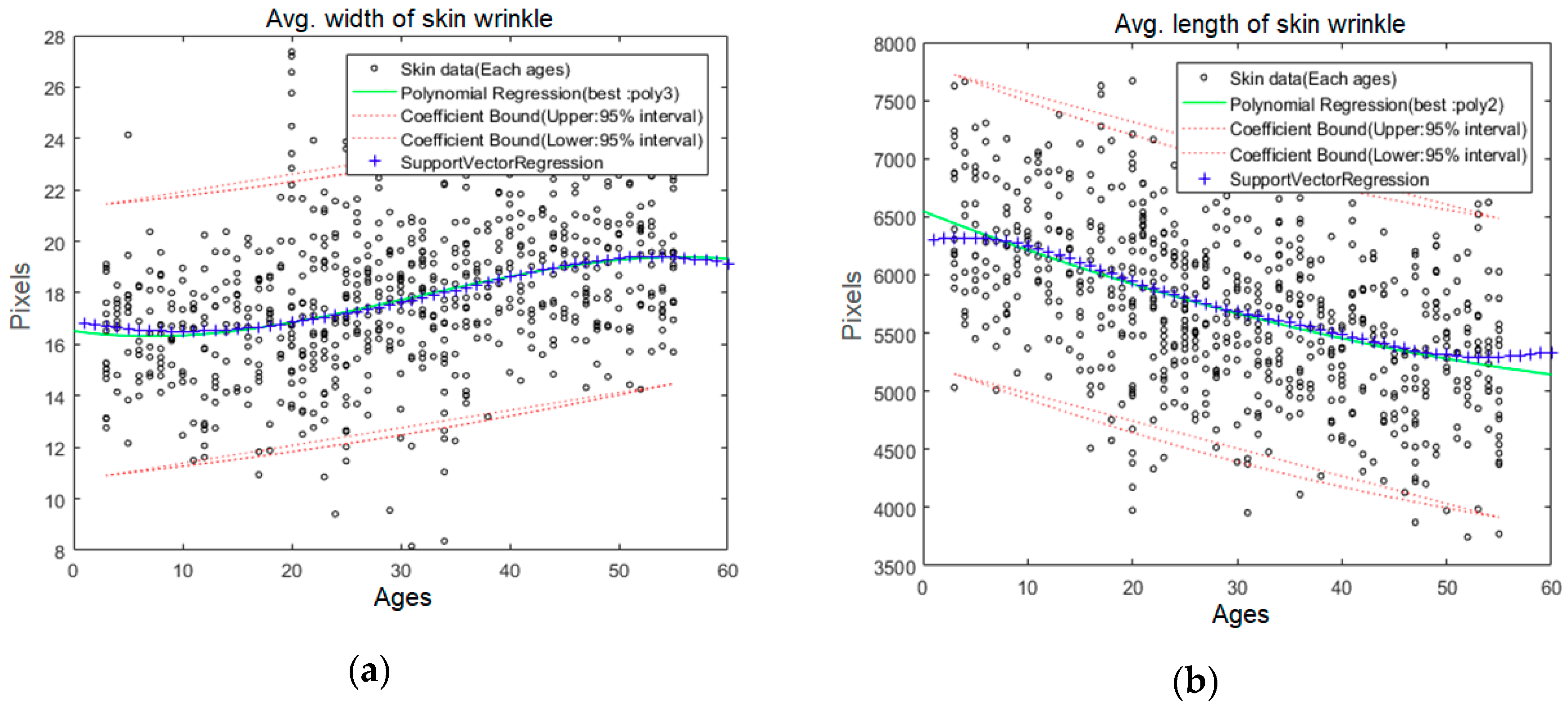
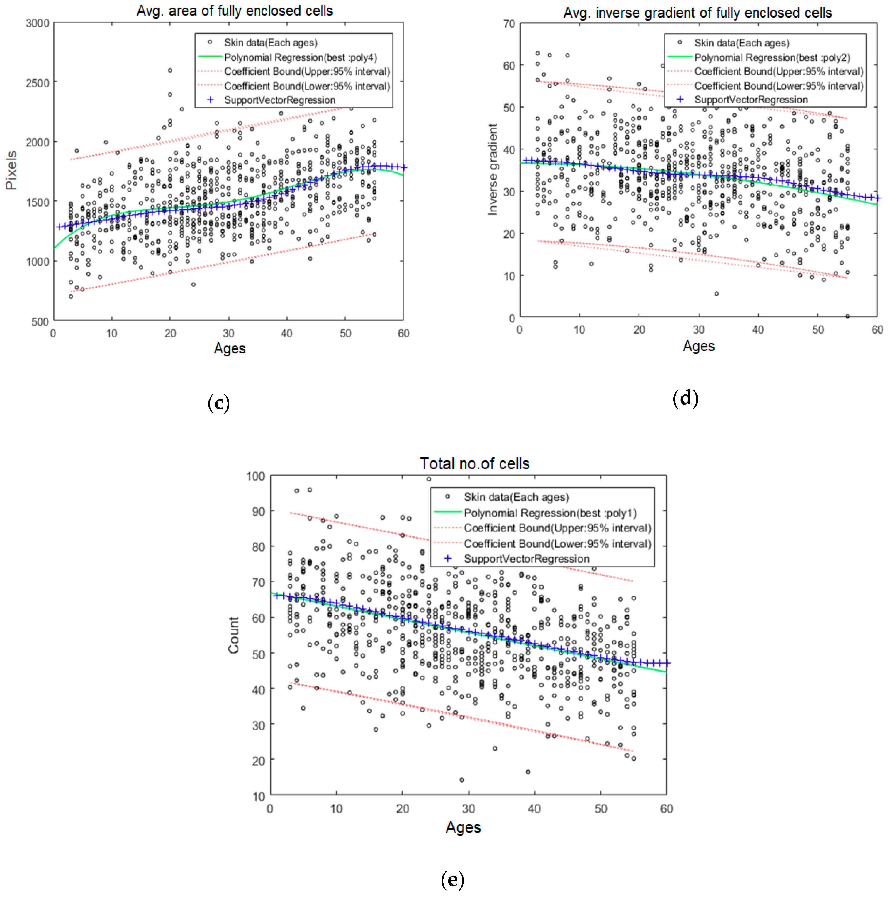
Figure 12, Figure 13 and Figure 14 show the skin aging estimation trends of overall face, neck, and hand. For skin texture aging trend estimation, we again extracted five texture features, which are skin wrinkle length, width, cell count, average cell area, and inverse gradient of cells. Based on these skin texture features, we estimated the skin texture aging trends using polynomial regression and SVR models. The green line indicates the polynomial regression estimation, which has the minimum SSE and root mean square error (RMSE). The blue and red dotted lines indicate the SVR estimation result and coefficient bound with 95% interval, respectively. The graphs in each of these figures depict the skin texture features distribution and their polynomial regression and SVR. Following our observation, the total length of skin wrinkle, average of inverse gradient of fully enclosed cells, and total number of cells decreased with age. The average of skin wrinkle width and average area of fully enclosed cells increased with age. Interestingly, the average of inverse gradient of fully enclosed face cells decreased considerably compared to the neck and hand. Similarly, the estimation trend of the total number of cells decreased considerably.
3.4. Correlation Analysis between Skin Texture and Life Pattern Changes
Table 2, Table 3, Table 4 and Table 5 show the Pearson correlation coefficients between the skin texture features and life activity of each of the four subjects. For skin texture aging coefficient analysis, we traced the lifestyle of each subject. We collected the life activity data using a questionnaire form that includes BMR questions, amount of sleeping time, eating meals, sun exposure times, drinking, and smoking. The investigated activity categories were studied to provide significant changes in skin condition changes [12,27,30]. During eight weeks, we observed daily the subject’s skin images and life activity changes.
Table 2 presents Pearson correlation analysis results from subject 1. Among the Pearson correlation results, sun exposure time and amount of drinking are significantly correlated with wrinkle length, wrinkle width, and sleeping time changes. In addition, sleeping time has a negative correlation with texture width changes, and drinking has a positive correlation with cell area changes. In summary, in the case of subject 1, the accumulated lack of sleeping time, the amount of sun exposure time, and drinking increased the wrinkle width and decrease the wrinkle length.
Table 3 presents Pearson correlation analysis results from subject 2, according to which correlation of sleeping time and skin texture features had the most positive correlation coefficient as compared to other correlation results. We observed a positive correlation of average wrinkle length and total number of cell features. On the contrary, the amount of drinking had an inverse correlation with wrinkle length and the average total number of cells. Subject 2’s significant correlation is detected in drinking activities.
Table 4 presents Pearson correlation analysis results for subject 3. The cell area, wrinkle length, and total number of cells had a significant correlation with sleeping time. Especially, subject 3’s feature changes were highly correlated with sleeping time. Lack of sleeping lead to decreased wrinkle width and cell area. The changes in BMR were correlated with average wrinkle width and length. We considered that these skin features are affected by BMR.
Table 5 indicates Pearson correlation analysis results for subject 4. Subject 4’s average wrinkle width, cell gradient, and total number of cells were significantly correlated with the accumulated sun exposure time. Especially, average wrinkle width and cell gradient had a positive correlation with accumulated sun exposure time. On the contrary, the average wrinkle length was positively correlated with sleeping time and the total number of cells was negatively correlated with the accumulated amount of drinking.
3.5. Simulation of Skin Texture Aging
Figure 15a shows the example of subject 1’s face texture aging simulation. To estimate the skin aging of subject 1, we considered subject 1 correlations results and applied the modified SDS values. The changes of subject 1 skin condition were most influenced by the amount of sleeping, sun light exposure and drinking, we modified SDS values of each activity (e.g., ‘negative’ activity value as 1, ‘normal’ activity value as 0.5 and ‘positive’ value as 0). Then, we applied these values to Equation (4) as an input. If subject 1 conducted negative activities on skin condition, his/her wrinkle width would be wider and the wrinkle length would be shorter than the current age. On the contrary, if subject 1 conducted positive life activities, his/her skin texture would maintain the current skin condition.
Figure 15b shows an example of subject 2’s face texture aging simulation. Subject 2’s skin condition was sensitive to accumulate sleeping and drinking. If subject 2 conducted heavy drinking and lack of sleeping, skin aging would accelerate. To apply the personal characteristics, we simulated in the same way as subject 1. Through the simulation process, we can observe the skin aging progress of subject 2’s face.
Figure 15c shows an example of subject 3’s face texture aging simulation. We observed that subject 3 changes of skin condition had correlated with food intakes and sleeping time. To reflect the personal characteristics, we modified the SDS of eating and sleeping activities. From the Pearson correlation results, we observed that subject 3’s skin condition, as well as lifestyle, changes. Subject 3’s skin was sensitive to the accumulated sleeping time and food intake. Figure 15d shows examples of subject 4’s skin texture changes in the simulation results. From the correlation results, we observed that subject 4’s skin condition was sensitive to the accumulated sun exposure time and amount of sleeping time. We can observe the progress of subject 4’s skin texture changes through simulation progress.
4. Conclusions
In this paper, we proposed a new scheme for tracing skin condition, estimating texture aging trend, and simulating skin aging. For an organized skin texture aging estimation model, we extracted diverse features which included skin texture width, length, cell, number of cells, and their areas. Based on the extracted skin texture features, we constructed the skin texture aging regression model and simulated the skin aging progress. In addition, we collected and analyzed the subject’s lifestyle, e.g, variation in sleeping time, amount of UV exposure, and amount of calories. Using the Pearson correlation method, we found the relation between skin texture aging and lifestyle. Based on the correlation results, we simulated the future skin texture aging. Our proposed scheme can be used for measuring the degree of skin damage, estimating skin aging, and simulating the process of skin aging.
In order to analyze the visual skin condition quantitatively, we plan to utilize more dataset and develop more efficient image processing algorithms to represent the characteristic of visual skin aging. To overcome the dataset quantity issue, we will consider the open datasets or collaborative research with clinical skin research centers. Since skin condition changes slowly over time, a further study with more focus on observing long-term changes of skin texture and life patterns should be done to understand what kinds of accumulated activities cause personal skin aging.
Author Contributions
Conceptualization, J.R. and Y.C.; investigation, H.K.; methodology, J.R. and Y.C.; software, J.R.; visualization, J.R.; writing—original draft preparation, J.R.; writing—review and editing, E.H.; supervision, E.H.;
Funding
This research was supported by the Brain Korea 21 Plus Project in 2019, and by the Basic Science Research Program through the National Research Foundation of Korea (NRF) funded by the Ministry of Education (NRF-2016R1D1A1A09919590).
Conflicts of Interest
The authors declare no conflict of interest.
References
- Cula, G.O.; Bargo, P.R.; Nkengne, A.; Kollias, N. Assessing facial wrinkles: Automatic detection and quantification. Skin Res. Technol. 2013, 19, 243–251. [Google Scholar] [CrossRef]
- Masuda, Y.M.; Oguri, T.; Morinaga, T.; Hirao, T. Three-dimensional morphological characterization of the skin surface micro-topography using a skin replica and changes with age. Skin Res. Technol. 2014, 20, 299–306. [Google Scholar] [CrossRef] [PubMed]
- Yow, A.P.; Cheng, J.; Li, A.; Srivastava, R.; Liu, J.; Wong, D.W.K.; Tey, H.L. Automated in vivo 3D high-definition optical coherence tomography skin analysis system. In Proceedings of the 2016 38th Annual International Conference of the IEEE Engineering in Medicine and Biology Society (EMBC), Orlando, FL, USA, 16–20 August 2016; pp. 3895–3898. [Google Scholar]
- Pirisinu, M.; Mazzarello, V. 3D profilometric characterization of the aged skin surface using a skin replica and alicona Mex software. Scanning 2016, 38, 213–220. [Google Scholar] [CrossRef] [PubMed]
- Kim, D.H.; Rhyu, Y.S.; Ahn, H.H.; Hwang, E.; Uhm, C.S. Skin microrelief profiles as a cutaneous aging index. J. Electron. Microsc. 2016, 65, 407–414. [Google Scholar] [CrossRef] [PubMed]
- Tanaka, H.; Nakagami, G.; Sanada, H.; Sari, Y.; Kobayashi, H.; Kishi, K.; Konya, C.; Tadaka, E. Quantitative evaluation of elderly skin based on digital image analysis. Skin Res. Technol. 2008, 14, 192–200. [Google Scholar] [CrossRef]
- Hamer, M.A.; Jacobs, L.C.; Lall, J.S.; Wollstein, A.; Hollestein, L.M.; Rae, A.R.; Gossage, K.W.; Hofman, A.; Liu, F.; Kayser, M.; et al. Validation of image analysis techniques to measure skin aging features from facial photographs. Skin Res. Technol. 2015, 21, 392–402. [Google Scholar] [CrossRef]
- Zou, Y.; Song, E.; Jin, R. Age-dependent changes in skin surface assessed by a novel two-dimensional image analysis. Skin Res. Technol. 2009, 15, 399–406. [Google Scholar] [CrossRef]
- Trojahn, C.; Dobos, G.; Schario, M.; Ludriksone, L.; Blume-Peytavi, U.; Kottner, J. Relation between skin micro-topography, roughness, and skin age. Skin Res. Technol. 2015, 21, 69–75. [Google Scholar] [CrossRef] [PubMed]
- Hames, S.C.; Ardigò, M.; Soyer, H.P.; Bradley, A.P.; Prow, T.W. Anatomical skin segmentation in reflectance confocal microscopy with weak labels. In Proceedings of the 2015 International Conference on Digital Image Computing: Techniques and Applications (DICTA), Adelaide, Australia, 23–25 November 2015; pp. 1–8. [Google Scholar]
- Xie, J.; Zhang, L.; You, J.; Zhang, D.; Qu, X. A study of hand back skin texture patterns for personal identification and gender classification. Sensors 2012, 12, 8691–8709. [Google Scholar] [CrossRef] [PubMed]
- Farage, M.A.; Miller, K.W.; Elsner, P.; Maibach, H.I. Intrinsic and extrinsic factors in skin ageing: A review. Int. J. Cosmet. Sci. 2008, 30, 87–95. [Google Scholar] [CrossRef]
- Gao, Q.; Yu, J.; Wang, F.; Ge, T.; Hu, L.; Liu, Y. Automatic measurement of skin textures of the dorsal hand in evaluating skin aging. Skin Res. Technol. 2013, 19, 145–151. [Google Scholar] [CrossRef] [PubMed]
- Miyamoto, K.; Nagasawa, H.; Inoue, Y.; Nakaoka, K.; Hirano, A.; Kawada, A. Development of new in vivo imaging methodology and system for the rapid and quantitative evaluation of the visual appearance of facial skin firmness. Skin Res. Technol. 2013, 19, 525–531. [Google Scholar] [CrossRef] [PubMed]
- Haluza, D.; Simic, S.; Moshammer, H. Sun exposure prevalence and associated skin health habits: Results from the Austrian population-based UVSkinRisk survey. Int. J. Environ. Res. Public Health 2016, 13, 141. [Google Scholar] [CrossRef] [PubMed]
- Krutmann, J.; Bouloc, A.; Sore, G.; Bernard, B.A.; Passeron, T. The skin aging exposome. J. Dermatol. Sci. 2017, 85, 152–161. [Google Scholar] [CrossRef] [Green Version]
- Tobin, D.J. Introduction to skin aging. J. Tissue Viability 2017, 26, 37–46. [Google Scholar] [CrossRef] [PubMed] [Green Version]
- Gunn, D.A.; Dick, J.L.; Van Heemst, D.; Griffiths, C.E.M.; Tomlin, C.C.; Murray, P.G.; Slagboom, P.E. Lifestyle and youthful looks. Br. J. Dermatol. 2015, 172, 1338–1345. [Google Scholar] [CrossRef]
- Park, S.Y.; Byun, E.; Lee, J.; Kim, S.; Kim, H. Air Pollution, Autophagy, and Skin Aging: Impact of Particulate Matter (PM10) on Human Dermal Fibroblasts. Int. J. Mol. Sci. 2018, 19, 2727. [Google Scholar] [CrossRef] [PubMed]
- Yang, H.; Huang, D.; Wang, Y.; Wang, H.; Tang, Y. Face aging effect simulation using hidden factor analysis joint sparse representation. IEEE Trans. Image Process. 2016, 25, 2493–2507. [Google Scholar] [CrossRef]
- Suo, J.; Zhu, S.C.; Shan, S.; Chen, X. A compositional and dynamic model for face aging. IEEE Trans. Pattern Anal. Mach. Intell. 2010, 32, 385–401. [Google Scholar] [PubMed]
- van Waateringe, R.P.; Slagter, S.N.; van der Klauw, M.M.; van Vliet-Ostaptchouk, J.V.; Graaff, R.; Paterson, A.D.; Wolffenbuttel, B.H. Lifestyle and clinical determinants of skin autofluorescence in a population-based cohort study. Eur. J. Clin. Investig. 2016, 46, 481–490. [Google Scholar] [CrossRef] [PubMed]
- Nam, Y.; Rho, S.; Lee, S. Extracting and visualising human activity patterns of daily living in a smart home environment. IET Commun. 2011, 5, 2434–2442. [Google Scholar] [CrossRef]
- Kim, K.; Choi, Y.H.; Hwang, E. Wrinkle feature-based skin age estimation scheme. In Proceedings of the IEEE International Conference on Multimedia and Expo, ICME 2009, New York, NY, USA, 28 June–3 July 2009; pp. 1222–1225. [Google Scholar]
- Choi, Y.H.; Tak, Y.; Rho, S.; Hwang, E. Skin feature extraction and processing model for statistical skin age estimation. Multimed. Tools Appl. 2013, 64, 227–247. [Google Scholar] [CrossRef]
- Choi, Y.H.; Kim, D.; Hwang, E.; Kim, B.J. Skin texture aging trend analysis using dermoscopy images. Skin Res. Technol. 2014, 20, 486–497. [Google Scholar] [CrossRef] [PubMed]
- Rew, J.; Choi, Y.H.; Rho, S.; Hwang, E. Monitoring skin condition using life activities on the SNS user documents. Multimed. Tools Appl. 2018, 77, 9827–9847. [Google Scholar] [CrossRef]
- Lowe, D.G. Distinctive image features from scale-invariant keypoints. Int. J. Comput. Vis. 2004, 60, 91–110. [Google Scholar] [CrossRef]
- Wu, F.L.; Fang, X.Y. An improved RANSAC homography algorithm for feature based image mosaic. In Proceedings of the 7th WSEAS International Conference on Signal Processing, Computational Geometry & Artificial Vision, Athens, Greece, 24–26 August 2007; pp. 202–207. [Google Scholar]
- Rew, J.; Choi, Y.H.; Kim, D.; Rho, S.; Hwang, E. Evaluating skin Hereditary traits based on daily activities. Front. Innov. Future Comput. Commun. 2014, 261–270. [Google Scholar]
Figure 1.
Examples of skin texture mapping step—(a) source image; (b) target image; (c) N grid partitioning; (d) grid mapping; (e) SIFT feature matching on K grids; (f) NCC matching on target image; (g) overlapped the mapped grids; (h) warped ROI.
Figure 1.
Examples of skin texture mapping step—(a) source image; (b) target image; (c) N grid partitioning; (d) grid mapping; (e) SIFT feature matching on K grids; (f) NCC matching on target image; (g) overlapped the mapped grids; (h) warped ROI.

Figure 2.
Examples of skin texture extraction step—(a) original image with ROI; (b) wrinkle and cell detection; (c) recovered wrinkle width; (d) wrinkle cell gradients.
Figure 2.
Examples of skin texture extraction step—(a) original image with ROI; (b) wrinkle and cell detection; (c) recovered wrinkle width; (d) wrinkle cell gradients.

Figure 3.
Flowchart of skin aging simulation.

Figure 4.
Cell and wrinkle regions clustering using L*a*b* color space and K-means (K = 5)—(a) cell; (b) wrinkle.
Figure 4.
Cell and wrinkle regions clustering using L*a*b* color space and K-means (K = 5)—(a) cell; (b) wrinkle.

Figure 5.
Cell and wrinkle color translation—(a) original; (b) cell color translation; (c) wrinkle color translation; (d) merged.
Figure 5.
Cell and wrinkle color translation—(a) original; (b) cell color translation; (c) wrinkle color translation; (d) merged.

Figure 6.
Wrinkle width expansion—(a) before wrinkle width expansion; (b) after wrinkle width expansion.
Figure 6.
Wrinkle width expansion—(a) before wrinkle width expansion; (b) after wrinkle width expansion.

Figure 7.
Example of cell vector expansion—(a) cell vector; (b) cell vector expansion.

Figure 8.
Cell vector expansion results—(a) merged image; (b) cell vector expansion; (c) cell vector; (d) expanded cell vector.
Figure 8.
Cell vector expansion results—(a) merged image; (b) cell vector expansion; (c) cell vector; (d) expanded cell vector.

Figure 9.
Application interface for skin aging simulation.

Figure 10.
Examples of skin dataset—(a) source image; (b) warping regions existing; (c) warping regions not existing.
Figure 10.
Examples of skin dataset—(a) source image; (b) warping regions existing; (c) warping regions not existing.

Figure 11.
Example of ROI warping results—(a) matched case; (b) non-matched case.

Figure 12.
Face skin texture aging trend estimation using polynomial regression and SVR—(a) average width trend of face wrinkle; (b) average length trend of face wrinkle; (c) average area trend of fully enclosed face cells; (d) average inverse gradient trend of fully enclosed face cells; (e) trend of the total number of face cells.


Figure 13.
Neck skin texture aging trend estimation using polynomial regression and SVR—(a) average width trend of neck wrinkle; (b) average length trend of neck wrinkle; (c) average area trend of fully enclosed neck cells; (d) average inverse gradient trend of fully enclosed neck cells; (e) trend of the total number of neck cells.


Figure 14.
Hand skin texture aging trend estimation using polynomial regression and SVR—(a) average width trend of hand wrinkle; (b) average length trend of hand wrinkle; (c) average area trend of fully enclosed hand cells; (d) average inverse gradient trend of fully enclosed hand cells; (e) trend of the total number of hand cells.


Figure 15.
Results of skin texture aging simulation—(a) subject #1’s face aging; (b) subject #2’s face aging; (c) subject #3’s face aging; (d) subject #4’s face aging.
Figure 15.
Results of skin texture aging simulation—(a) subject #1’s face aging; (b) subject #2’s face aging; (c) subject #3’s face aging; (d) subject #4’s face aging.


Table 1.
Average accuracy of ROI warping.
| Dataset | Avg. Warping Accuracy (No. of grids = 4) | Avg. Warping Accuracy (No. of grids = 48) | Avg. Warping Accuracy (No. of grids = 108) |
|---|---|---|---|
| Face | 81.32% | 86.57% | 91.43 % |
| Hand | 83.74% | 87.26% | 92.88% |
| Neck | 72.54% | 74.21% | 78.52% |
Table 2.
Pearson correlation coefficient (subject 1).
| Life Activity | Avg. Wrinkle Width (px) | Avg. Length of Wrinkle (px) | Avg. Cell Area (px) | Avg. Cell Gradient (Degrees) | Total No. of Cell (# Cells) |
|---|---|---|---|---|---|
| Sleeping time | −0.282 | 0.197 | −0.182 | −0.101 | 0.182 |
| BMR | 0.132 | 0.135 | 0.152 | 0.087 | 0.105 |
| Sun exposure time | 0.217 | −0.242 | 0.174 | 0.052 | −0.188 |
| Drinking | 0.321 | −0.281 | 0.284 | 0.131 | −0.211 |
| Amount of smoking | 0.138 | −0.116 | 0.102 | 0.125 | −0.123 |
Table 3.
Pearson correlation coefficient (subject 2).
| Life Activity | Avg. Wrinkle Width (px) | Avg. Length of Wrinkle (px) | Avg. Cell Area (px) | Avg. Cell Gradient (Degrees) | Total No. of Cell (# Cells) |
|---|---|---|---|---|---|
| Sleeping time | −0.185 | 0.218 | −0.144 | −0.178 | 0.092 |
| BMR | 0.101 | 0.105 | 0.116 | 0.135 | 0.113 |
| Sun exposure time | 0.147 | −0.142 | 0.201* | 0.073 | −0.105 |
| Drinking | 0.121 | −0.235 | 0.213 | 0.111 | −0.217 |
| Amount of smoking | - | - | - | - | - |
Table 4.
Pearson correlation coefficient (subject 3).
| Life Activity | Avg. Wrinkle Width (px) | Avg. Length of Wrinkle (px) | Avg. Cell Area (px) | Avg. Cell Gradient (Degrees) | Total No. of Cell (# Cells) |
|---|---|---|---|---|---|
| Sleeping time | −0.318 | 0.232 | −0.219* | −0.182 | 0.287 |
| BMR | 0.208 | 0.210* | 0.181 | 0.158 | 0.172 |
| Sun exposure time | 0.121 | −0.118 | −0.089 | 0.097 | −0.085 |
| Drinking | −0.078 | −0.086 | 0.108 | 0.108 | −0.113 |
| Amount of smoking | - | - | - | - | - |
Table 5.
Pearson correlation coefficient (subject 4).
| Life Activity | Avg. Wrinkle Width (px) | Avg. Length of Wrinkle (px) | Avg. Cell Area (px) | Avg. Cell Gradient (Degrees) | Total No. of Cell (# Cells) |
|---|---|---|---|---|---|
| Sleeping time | −0.146 | 0.208* | −0.107 | −0.085 | 0.124 |
| BMR | 0.152 | 0.121 | 0.157 | 0.133 | 0.146 |
| Sun exposure time | 0.287* | −0.198 | 0.154 | 0.205* | −0.228* |
| Drinking | 0.158 | −0.116 | 0.138 | 0.128 | −0.223* |
| Amount of smoking | - | - | - | - | - |
© 2019 by the authors. Licensee MDPI, Basel, Switzerland. This article is an open access article distributed under the terms and conditions of the Creative Commons Attribution (CC BY) license (http://creativecommons.org/licenses/by/4.0/).
Share and Cite
MDPI and ACS Style
Rew, J.; Choi, Y.-H.; Kim, H.; Hwang, E. Skin Aging Estimation Scheme Based on Lifestyle and Dermoscopy Image Analysis. Appl. Sci. 2019, 9, 1228. https://doi.org/10.3390/app9061228
AMA Style
Rew J, Choi Y-H, Kim H, Hwang E. Skin Aging Estimation Scheme Based on Lifestyle and Dermoscopy Image Analysis. Applied Sciences. 2019; 9(6):1228. https://doi.org/10.3390/app9061228
Chicago/Turabian StyleRew, Jehyeok, Young-Hwan Choi, Hyungjoon Kim, and Eenjun Hwang. 2019. "Skin Aging Estimation Scheme Based on Lifestyle and Dermoscopy Image Analysis" Applied Sciences 9, no. 6: 1228. https://doi.org/10.3390/app9061228
Note that from the first issue of 2016, this journal uses article numbers instead of page numbers. See further details here.