Evidence-Theory-Based Robust Optimization and Its Application in Micro-Electromechanical Systems


1
School of Mechanical and Electrical Engineering, Hunan City University, Yiyang 413002, China
2
College of Mechanical and Vehicle Engineering, Hunan University, Changsha 40082, China
3
School of Vehicle and Mechanical Engineering, Changsha University of Science and Technology, Changsha 410076, China
*
Author to whom correspondence should be addressed.
Appl. Sci. 2019, 9(7), 1457; https://doi.org/10.3390/app9071457
Submission received: 21 February 2019
/
Revised: 30 March 2019
/
Accepted: 1 April 2019
/
Published: 7 April 2019
(This article belongs to the Special Issue Advanced Theoretical and Computational Methods for Complex Materials and Structures)
Abstract
:Featured Application
This paper develops an evidence-theory-based robustness optimization (EBRO) method, which aims to provide a potential computational tool for engineering problems with epistemic uncertainty. This method is especially suitable for robust designing of micro-electromechanical systems (MEMS). On one hand, unlike traditional engineering structural problems, the design of MEMS usually involves micro structure, novel materials, and extreme operating conditions, where multi-source uncertainties inevitably exist. Evidence theory is well suited to deal with such uncertainties. On the other hand, high performance and insensitivity to uncertainties are the fundamental requirements for MEMS design. The robust optimization can improve performance by minimizing the effects of uncertainties without eliminating these causes.
Abstract
The conventional engineering robustness optimization approach considering uncertainties is generally based on a probabilistic model. However, a probabilistic model faces obstacles when handling problems with epistemic uncertainty. This paper presents an evidence-theory-based robustness optimization (EBRO) model and a corresponding algorithm, which provide a potential computational tool for engineering problems with multi-source uncertainty. An EBRO model with the twin objectives of performance and robustness is formulated by introducing the performance threshold. After providing multiple target belief measures (Bel), the original model is transformed into a series of sub-problems, which are solved by the proposed iterative strategy driving the robustness analysis and the deterministic optimization alternately. The proposed method is applied to three problems of micro-electromechanical systems (MEMS), including a micro-force sensor, an image sensor, and a capacitive accelerometer. In the applications, finite element simulation models and surrogate models are both given. Numerical results show that the proposed method has good engineering practicality due to comprehensive performance in terms of efficiency, accuracy, and convergence.
1. Introduction
In practical engineering problems, various uncertainties exist in terms of the operating environment, manufacturing process, material properties, etc. Under the combined action of these uncertainties, the performance of engineering structures or products may fluctuate greatly. Robust optimization [1,2] is a methodology, and its fundamental principle is to improve the performance of a product by minimizing the effects of uncertainties without eliminating these causes. The concept of robustness optimization has long been embedded in engineering design. In recent years, thanks to the rapid development of computer technology, it has been widely applied to many engineering fields, such as electronic [3], vehicle [4], aerospace [5], and civil engineering [6]. The core of robustness optimization lies in understanding, measuring, and controlling the uncertainty in the product design process. In mechanical engineering disciplines, uncertainty is usually differentiated into objective and subjective from an epistemological perspective [7]. The former, also called aleatory uncertainty, comes from an inherently irreducible physical nature, e.g., material properties (elasticity modulus, thermal conductivity, expansion coefficient) and operating conditions (temperature, humidity, wind load). A probabilistic model [8,9,10] is an appropriate way to describe such uncertain parameters, provided that sufficient samples are obtained for the construction of accurate random distribution. Conventional robustness optimization methods [11,12,13] are based on probabilistic models, in which the statistical moments (e.g., mean, variance) are employed to formulate the robustness function for the performance assessment under uncertainties. On the other hand, designers may lack knowledge about the issues of concern in practice, which leads to subjective uncertainty, also known as epistemic uncertainty. The uncertainty is caused by cognitive limitation or a lack of information, which could be reduced theoretically as effort is increased. At present, the methods of dealing with epistemic uncertainty mainly include possibility theory [14,15], the fuzzy set [16,17], convex model [18,19], and evidence theory [20,21]. Among them, evidence theory is an extension of probability theory, which can properly model the information of incompleteness, uncertainty, unreliability and even conflict [22]. When evidence theory treats a general structural problem, all possible values of an uncertain variable are assigned to several sub-intervals, and the corresponding probability is assigned to each sub-interval according to existing statistics and expert experience. After synthesizing the probability of all the sub-intervals, the belief measure and plausibility measure are obtained, which constitute the confidence interval of the proposition and show that the structural performance satisfies a given requirement. Compared with other uncertainty analysis theories, evidence theory may be more general. For example, when the sub-interval of each uncertain variable is infinitely small, evidence theory is equivalent to probability theory; when the sub-interval is unique, it is equivalent to convex model theory; when no conflict occurs to the information from different sources, it is equivalent to possibility theory [23].
In the past decade, some progress has been made in evidence-theory-based robust optimization (EBRO). For instance, Vasile [24] employed evidence theory to model the uncertainties of spacecraft subsystems and trajectory parameters in the robust design of space trajectory and presented a hybrid co-evolutionary algorithm to obtain the optimal results. For the preliminary design of a space mission, Croisard et al. [25] formulated the robust optimization model using evidence theory and proposed three practical solving technologies. Their features of efficiency and accuracy were discussed through the application of a space mission. Zuiani et al. [26] presented a multi-objective robust optimization approach for the deflection action design of near-Earth objects, and the uncertainties involved in the orbital and system were qualified by evidence theory. A deflection design application of a spacecraft swarm with Apophis verified the effectiveness of this approach. Hou et al. [27] introduced evidence-theory-based robust optimization (EBRO) into multidisciplinary aerospace design, and the strategy of an artificial neural network was used to establish surrogate models for the balance of efficiency and accuracy during the optimization. This method was applied to two preliminary designs of the micro entry probe and orbital debris removal system. The above studies employed evidence theory to measure the epistemic uncertainties involved in engineering design, and expanded robustness optimization into the design of complex systems. However, the studies of EBRO are still in a preliminary stage. The existing research has mainly aimed at the preliminary design of engineering systems. Most of them have been simplified and assumed to a great extent. In other words, the performance functions are based on surrogate models and even empirical formulas. So far, EBRO applications in actual product design, with a time-consuming simulation model being created for performance function, are actually quite few. After all, computational cost is a major technical bottleneck limiting EBRO applications. First, evidence theory describes uncertainty through a series of discontinuous sets, rather than a continuous function similar to a probability density function. This usually leads to a combination explosion in a multidimensional robustness analysis, and finally results in a heavy computational burden. Secondly, EBRO is essentially a nested optimization problem with performance optimization in the outer layer and robustness analysis in the inner layer. The direct solving strategy means a large number of robustness evaluations using evidence theory. As a result, the issue of EBRO efficiency is further exacerbated. Therefore, there is a great engineering significance in developing an efficient EBRO method in view of actual product design problems.
In this paper, a general EBRO model and an efficient algorithm are proposed, which provide a computational tool for robust product optimization with epistemic uncertainty. The proposed method is applied to three design problems of MEMS, in which its engineering practicability is discussed. The remainder of this paper is organized as follows. Section 1 briefly introduces the basic concepts and principles of robustness analysis using evidence theory. The EBRO model is formulated Section 2. The corresponding algorithm is proposed in Section 3. In Section 4, this method is validated through the three applications of MEMS—a micro-force sensor, a low-noise image sensor and a capacitive accelerometer. Conclusions are drawn in Section 5.
2. Robustness Analysis Using Evidence Theory
Consider that uncertainty problem is given as , where Z represents the nZ-dimensional uncertain vector, f is the performance function which is uncertain due to Z. Conventional methods [16,17,18] of robust optimization employ probability theory to deal with the uncertainties. The typical strategy is to consider the uncertain parameters of a problem as random variables, and thereby the performance value is also a random variable. The mean and variance are used to formulate the robustness model. In practical engineering, it is sometimes hard to construct accurate probability models due to the limited information. Thus, evidence theory [20,21] is adopted to model the robustness. In evidence theory, the frame of discernment (FD) needs to be established first, which contains several independent basic propositions. It is similar to the sample space of a random parameter in probability theory. Here, denotes the power set of the FD (namely ), and consists of all possible propositions contained in . For example, for a FD with the two basic propositions of and , the corresponding power set is . Evidence theory adopts a basic probability assignment (BPA) to measure the confidence level of each proposition. For a certain proposition A, the BPA is a mapping function that satisfies the following axioms:
where if , A is called a focal element of m. The BPA of denotes the extent to which the evidence supports Proposition A. When the information comes from multiple sources, can be obtained by evidence combination rules [28]. Evidence theory uses an interval consisting of the belief measure (Bel) and the plausibility measure (Pl) to describe the true extent of the proposition. The two measures are defined as:
As can be seen from Equation (2), is the summary of all the BPA that totally support Proposition A, while is the summary of the BPA that support Proposition A totally or partially.
A two-dimensional design problem is taken as the example to illustrate the process of robustness analysis using evidence theory. The performance function contains two uncertain parameters , which are both considered as evidence variables. The FDs of a, b are the two closed intervals, i.e., and . A contains nA number of focal elements, and the subinterval of represents the i-th focal element of A. The definitions of and are similar. Thus, a Cartesian product can be constructed:
where is the k-th focal element of D, and the total number of focal elements is . For ease of presentation, assuming that a, b are independent, a two-dimensional joint BPA is obtained:
More general problems with parametric correlation can be handled using the mathematical tool of copula functions [29].
As analyzed above, the performance function of f is uncertain. The performance threshold of v is given to evaluate its robustness. Given that the design objective is to minimize the value of f, the higher the trueness of Proposition , the higher the robustness of f relative to v. Proposition is defined as the feasible domain:
Substituting A, C with F, in Equation (2), the belief measure and plausibility measure of Proposition are expressed as follows:
In evidence theory, the probabilistic interval composed by the two measures can describe the trueness of , written as . The accumulation of needs to determine the positional relationship between each focal element and the F domain. As a result, the performance function extrema of each focal element must be searched. For this example, the pairs of extremum problems are established as:
where , are the minimum and maximum of the k-th focal element. The vertex method [30] can efficiently solve the problems in Equation (7) one by one. If , , and is simultaneously accounted into and ; If , , and is only accounted into . After calculating the extrema for all focal elements, the and can be totaled.
3. Formulation of the EBRO Model
As mentioned above, evidence theory uses a pair of probabilistic values to measure the robustness of the performance value related to the given threshold. However, engineers generally tend to adopt conservative strategies to deal with uncertainties in the product design process. Thus, the robustness objective of EBRO can be established as . Meanwhile, in order to improve product performance, the performance threshold is minimized. The EBRO model is formulated as a double-objective optimization problem:
where d is the -dimensional deterministic design vector; X is the -dimensional uncertain design vector; P is the -dimensional uncertain parameter vector; the superscripts of l, u represent the value range of a design variable; and represents the nominal value of X. Note that the threshold of v is usually difficult to give a fixed value to, while it should be treated as a deterministic design variable.
The proposed model is an improvement on the existing model [24] because it can handle more types of uncertainty, such as the perturbations of design variables resulting from production tolerances, and the variations of parameters due to changing operating conditions. As for the solving process, the EBDO involves the nested optimization of the double-objective optimization in the outer layer and the robustness assessment in the inner layer. Due to the discreteness introduced by the evidence variables, each of the robustness analyses need to calculate the performance extrema of all focal elements. Essentially, extremum evaluation is an optimization problem involving the performance function based on time-consuming simulation models, and therefore the robustness analysis bears a high computational cost. More seriously, the double-objective optimization in the outer layer requires a large number of robustness evaluations in the inner layer. Eventually, the EBDO solving becomes extremely inefficient.
4. The Proposed Algorithm
To improve efficiency, this paper proposes a decoupling algorithm of EBRO, and its basic idea is to convert the nested optimization into the sequence iteration process. Firstly, the original problem is decomposed into a series of sub-problems. Secondly, the uncertainty analysis and the deterministic optimization are driven alternately until convergence. The framework of the proposed method is detailed below.
4.1. Decomposition into Sub-Problems
Robust optimization is essentially a multi-objective problem that increases product performance at the expense of its robustness. Therefore, robust optimization generally does not have a unique solution, but a set of solutions called the Pareto optimal set [2]. It is a family of solutions that is optimal in the sense that no improvement can be achieved in any objective without degradation in others for a multi-objective problem. The Pareto-optimal solutions can be obtained by solving appropriately formulated single objective optimization problems on a one-at-a-time basis. At present, a number of multi-objective genetic algorithms have been suggested. The primary reason for this is their ability to find multiple Pareto-optimal solutions in parallel. From the viewpoint of mathematical optimization, genetic algorithms are a kind of suitable method for solving a general multi-objective optimization. However, the efficiency of a genetic algorithm is usually much lower than the gradient-based optimization algorithms, which has become the main technical bottleneck limiting its practical application [31,32]. Although a priori information is not required when using genetic algorithms, most designers have some engineering experience in practice. Therefore, for the specific problem shown in Equation(8), the robustness objective of is often handled as a reliability constraint [2,33]. In this paper, the EBRO problem is transformed into a series of sub-problems under the given target belief measures:
where represents the j-th target belief measure; and is the reliability constraint derived from the robust objective. In many cases, the designer may focus on the performance values under some given conditions based on the experience or quality standard. This condition is usually a certain probability of , namely .
4.2. Iteration Framework
Theoretically, the EBDO problems in Equation (9) can be solved by existing methods [34]. However, the resulting computational burden will be extremely heavy. To address this issue, a novel iteration framework is developed, in which the uncertainty analysis and design optimization alternate until convergence.
In the k-th iteration, each optimization problem in Equation (9) requires the performance of an uncertainty analysis at the previous design point:
This mainly consists of two steps, illustrated by the example in Figure 1. Step 1 is to search for the most probable focal element (MPFE) along the limit-state boundary of . The MPFE [35] is similar to the most probable point (MPP) in probability theory, which is the point with the most probability density on the limit-state boundary. Compared to other points on the boundary, the minimal error of reliability analysis can be achieved by establishing the linear approximation for the performance function at the MPP [36]. Similarly, the MPFE contains the maximal BPA among the focal elements that are crossed by the limit-state boundary. The searching process of MPFE is formulated as:
where represents the BPA of the focal element where the Z point is located. Note that there is a difference between at each iteration step due to the minor difference of . Consequently, different MPFEs may be obtained for Equation (11). However, the difference between the MPFEs is minor relative to the entire design domain. To ensure efficiency, the unique MPFE is investigated at each iteration. Equation (11) can be rewritten as:
where represents the performance threshold that has not yet converged.
Step 2 is to establish linear approximation for the performance function at the central point of MPFE:
The L-function is used to replace the f-function to calculate Bel, and thereby the optimization processes in Equation (7) no longer requires the calculation of any performance function.
The efficient calculation of Bel has been achieved in the iterative process, but the overall process of EBDO still requires dozens or even hundreds of Bel evaluations due to the nested optimization. To eliminate the nested optimization, a decoupling strategy is proposed similar to that in the probabilistic method [37]. At each iteration step, the reliability constraint is transformed into a deterministic constraint by constructing the shifting vector of ; and then a deterministic optimization is updated and solved to obtain the current solution. In the k-th iteration, the deterministic optimization can be written as:
The shifting vector determines the deviation between the original reliability boundary and the deterministic boundary at the k-th iteration step. For the j-th problem in Equation (14), the formulation of the shifting vector is explained as in Figure 2. For convenience of presentation, the constraint contains only two evidence variables . F represents the domain of . is the previous design point, which is based on the previous equivalent boundary of . The rectangular domain represents the FD at the previous design point. F represents the domain of . If the FD is entirely in the F domain, . In Figure 2, the FD of is partially in the F domain, and is still less than . To satisfy , needs to move further into the F domain. Therefore, the equivalent boundary needs to move further toward the F domain. The updated equivalent boundary is constructed as follows:
where denotes the increment of the previous shifting vector. The principle for calculating is set as and is just satisfied. Thus, the mathematical model of is created as:
Equation (16) can be solved by multivariable optimization methods [38]. To further improve efficiency, the f -function is replaced by the L-function formulated in Equation (13).
Uncertain analysis and design optimization are carried out alternatively until they meet the following convergence criteria:
where is the minimal error limit. The solutions of form the final optimal set.
The flowchart of the EBRO algorithm is summarized as Figure 3.
5. Application Discussion
In the previous sections, an EBDO method is developed for engineering problems with epistemic uncertainty. This method is especially suitable for the robust design of micro-electromechanical systems (MEMS). On one hand, unlike traditional engineering structural problems, the design of MEMS usually involves micro structure, novel materials, and extreme operating conditions, where epistemic uncertainties inevitably exist. Evidence theory is well suited to deal with such uncertainties. On the other hand, high performance and insensitivity to uncertainties are the fundamental requirements for MEMS design. Over the past two decades, robust optimization for MEMS has gradually attracted the attention of both academics and engineering practice [39,40,41]. In this section, this method is applied to three applications of MEMS: a micro-force sensor, a low-noise image sensor, and a capacitive accelerometer. The features of the proposed approach are investigated in terms of efficiency and accuracy. Performance function evaluations are accounted to indicate efficiency, and the reference solution is compared to verify accuracy. The reference solution is obtained by the double-loop method, where sequential quadratic programming [38] is employed for performance optimization, and a Monte-Carlo simulation [42] is used for robust assessment.
5.1. A Micro-Force Sensor
A piezoelectric micro-force sensor [43] has several advantages, including a reliable structure, fast response, and simple driving circuits. It has been extensively applied in the fields of precision positioning, ultrasonic devices, micro-force measurement, etc. Given that uncertainties are inevitable in structural sizes and material parameters, robust optimization is essential to ensure the performance of the sensor.
As shown in Figure 4, the core part of the micro-force sensor is a piezoelectric cantilever beam, which consists of a piezoelectric film, a silicon-based layer, and two electrodes. The force at the free end causes bending deformation on the beam, which drives the piezoelectric film to output polarization charges through the piezoelectric effect. The charge is transmitted to the circuit by the electrodes and converted into a voltage signal. According to the theoretical model proposed by Smits et al. [43], this voltage can be formulated as:
where
where F is the concentration force; L, w represent the length and width of the beam; , denote the thickness of the silicon-base layer and piezoelectric film; , are the compliance coefficient of the silicon-based layer and piezoelectric film; and , is the piezoelectric coefficient and dielectric constant of the piezoelectric film. The constants in Equation (18) include , , and , The structural sizes of L, w, h and the material parameter of , are viewed as evidence variables. The marginal BPAs of the variables are shown in Figure 5, and the nominal values of , are, respectively, , .
In engineering, the greater the output voltage, the higher the theoretical accuracy of the sensor. Thus, U is regarded as the objective function. The design variables are and . The constraints of shape, stiffness and strength are considered, which are expressed as , , and , where is the ratio of w to h, denotes the displacement at the free end of the beam, and denotes the maximum stress of the beam. and can be written as [43].
Due to uncertainties in the structure, , and are also uncertain. Theoretically, the three constraints should be modeled as reliability constraints. To focus on the topic of robust optimization, the constraints are considered as deterministic in this example. That is, the nominal values of the uncertain variables are used to calculate , and . In summary, the EBRO problem is formulated as follows:
where ; represents the performance threshold, which is set as the deterministic design variable.
The steps to solve this problem using the proposed method are detailed below. Firstly, according to the marginal BPAs of the five variables in Figure 5, the joint BPAs of the focal elements (85 = 32768) are calculated by Equation (4). Secondly, Equation (21) is converted into a series of sub-problems, which are expressed as:
where represent a series of target Bel for the proposition of , which are given by the designer according to engineering experience or quality standards. Thirdly, the iteration starts from the initial point of , where are selected by the designer and is calculated by Equation (18). At each iteration step, the approximate function of U is established as Equation (13), and then 10 numbers of are obtained through Equation (16). Correspondingly, the 10 optimization problems as Equation (14) are updated. By solving them, the optimal set in the current iteration is obtained. After four iteration steps, the optimal set is converged as listed in Table 1. The results show that the performance threshold decreases gradually with increase in Bel. In engineering, a designer can intuitively select the optimal design option from the optimal set by balancing the product performance and robustness. In term of accuracy, the solutions of the proposed method are very close to the corresponding reference solutions, and the maximal error is only 2.5% under the condition of . In efficiency, the proposed method calculates performance function only 248 times, and the computational cost is much less than that of evolutionary algorithms [31]. From a mathematical point of view, it is unfair to compare the efficiency of the proposed method with the evolutionary algorithms. From the view of engineering practicality, however, the solutions of the proposed method may help the designers create a relatively clear picture of the problem with high efficiency and acceptable accuracy.
5.2. An Ultra-Low-Noise Image Sensor
Recently, a type of ultra-low-noise image sensor [44] was developed for applications requiring high-quality imaging under extremely low light conditions. Such a type of sensor is ideally suited for a variety of low light level cameras for surveillance, industrial, and medical applications. In application, the sensor and other components are assembled on a printed circuit board (PCB). Due to the mismatch in the thermal expansion coefficient of the various materials, thermal deformation occurs on the PCB under the combined action of self-heating and thermal environment. As a result, the imaging quality of the sensor is reduced. Moreover, to acquire more image information under low-light conditions, the sensor is designed in a large format. Thus, the imaging quality is more susceptible to deformation. This issue has become a challenging problem in this field and needs to be solved urgently.
A robust optimization problem is considered for the camera module as Figure 6, in which the image-sensor-mounted PCB is fastened with the housing. The sensor is designed as a 4/3-inch optical format and features an array of five transistor pixels on a 6.5 μm pitch with an active imaging area of pixels. It delivers extreme low light sensitivity with a read noise of less than 2.0 electrons root mean square (RMS) and a quantum efficiency above 55%. In order to analyze the thermal deformation of the sensor under the operating temperature , the finite element model (FEM) is created as shown in Figure 7, in which the power dissipation of the codec chip and the converter is given as 1.2 W and 0.2 W, according to the test data. It can be observed that a certain deformation appears on the sensor die, and the peak–peak value (PPV) of the displacement response achieves about 3.0 μm. Consequently, the image quality of the sensor will decrease. To address the issue, the design objective is set to minimize the PPV, and the design variables of are the normal positions of the PCB-fixed points. In engineering, manufacturing errors are unavoidable and power dissipation fluctuates with changing loads, and thereby X and P are treated as evidence variables. Their BPAs are summarized on the basis of limited samples, as listed in Table 2. This robust optimization is constructed as follows:
As mentioned above, the performance function of PPV is implicit and based on the time-consuming FEM, which consists of 88,289 8-node thermally coupled hexahedron elements. The computational time for solving the FEM is about 0.1 h, if using a computer with the i7-4710HQ CPU and 8 G of RAM. To realize the parameterization and reduce the computational cost of obtaining reference solutions, a second-order polynomial response surface is created for the performance function by sampling 200 times on the FEM.
In order to analyze the efficiency of the proposed method for problems with different dimensional uncertainty, three cases are considered: only P is uncertain in Case 1; only X is uncertain in Case 2; and both of them are uncertain in Case 3. The initial design option is selected as , and is obtained by . After giving , the original problem is converted into three sub-problems, as in Equation (9). They are solved by the proposed method and the double-loop method; all results are listed in Table 3. Firstly, the results of the proposed method and the reference solutions are almost identical for all cases, and thus the validity of the results is presented. Secondly, each of the cases converges into a stable optimal set after three or four iteration steps. For this problem, the convergence of the proposed method is little affected by the number of uncertain variables. Thirdly, the performance function evaluations increase with the increasing dimensional number of uncertainties, while overall the efficiency of the proposed method is relatively high. Case 3 is taken as an example. Even if the FEM is called directly by EBRO, means a computational time of only about 20 h.
5.3. A Capacitive Accelerometer
The capacitive accelerometer [45] has become very attractive for high-precision applications due to its high sensitivity, low power consumption, wide dynamic range of operation, and simple structure. The capacitive accelerometer is not only the central element of inertial guidance systems, but also has applications in a wide variety of industrial and commercial problems, including crash detection for vehicles, vibration analysis for industrial machinery, and hovering control for unmanned aerial systems.
Most of the capacitive accelerometers consist of two main modules: the sensing structure and the signal processing circuit; the former plays a critical role in the overall product performance. The sensing structure in this example, as in Figure 8, mainly includes five parts: a fixed electrode, a movable electrode, a coil, a counter weight, block 1, and block 2. The material they are made of is listed in Table 4. The capacitance between the two electrodes varies with the vertical displacement of the movable plate under the excitation of acceleration, which can be clearly presented through the finite element simulation, as in Figure 9. The nodes in the effective area on the movable electrode have been offset relative to the original position under the excitation of acceleration. The increment of capacitance is expressed as [44]:
where is the dielectric constant; h represents the original distance between the electrodes; S denotes the effective area on the movable electrode; is the displacement response of the i-th node, and is the area of corresponding element. Note that the performance function of A is based on the FEM, which contains 114,517 8-node thermally coupled hexahedron elements in total, and it takes about 1/3 h to solve each time, when using a personal computer. The displacement of the movable electrode, in addition to the response to acceleration, may be caused by varying ambient temperature. This can be found from the simulation result in Figure 9, where the load is changed from acceleration to varying temperature. Reducing the effect of thermal deformation on accuracy has become a problem that must be faced in the design process. Therefore, the EBRO model of the capacitive accelerometer is formulated as:
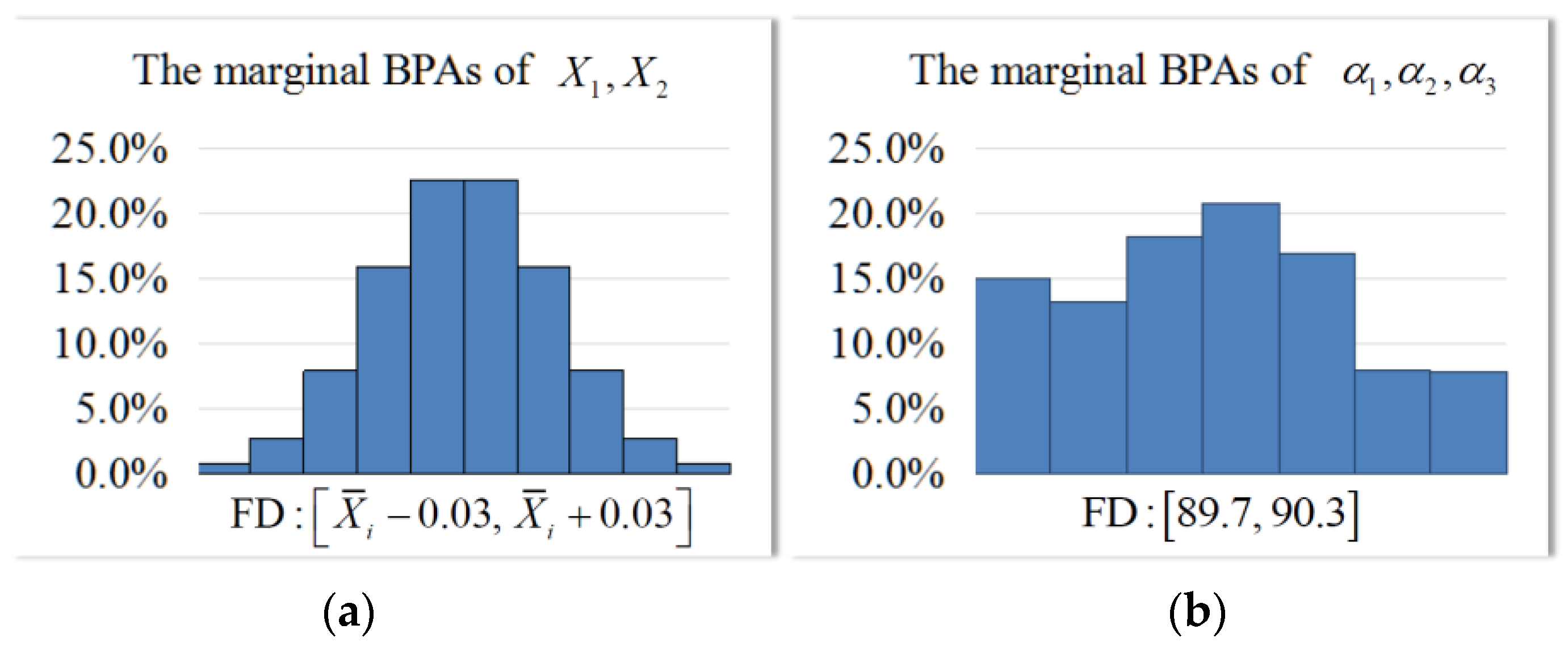
where f represents the sensitivity of error to temperature at 35 °C; v denotes the performance threshold; and X, P denote the design vector and parameter vector. The components of X, α are the structural sizes, as shown in Figure 8, where are the mounting angle of the counter weight, block 1 and block 2, respectively. The value ranges are given as , and the nominal values are . All of them are uncertain variables, respectively caused by machining errors and assembly errors. According to the existing samples, the marginal BPAs are listed in Figure 10.
After being given a series of , Equation (26) can be rewritten as Equation (27):
For easy reproduction of results, the response surface of is constructed as follows:
Next, the EBRO is performed by the proposed method and the double-loop method. The initial design point is selected as , and . All results are given in Table 5. The proposed method converges the optimal set after four iteration steps. Each element of the optimal set is very close to that of the reference solution. This indicates to some extent the convergence and accuracy of the proposed method. As for efficiency, the performance function evaluations of the proposed method are done 171 times. Compared to the double-loop method (12,842 times), the efficiency of this method has a definite advantage. Given that hundreds of simulations or dozens of hours of computation are acceptable for most engineering applications, it is feasible to directly call the time-consuming simulation model when performing the EBRO in practice.
On the other hand, the proposed method provides six design options under different robustness requirements in this example. The higher the robustness, the greater the performance threshold. From a designer’s point of view, choosing a lower yield (i.e., ) means that a higher cost and less error (i.e., ) are introduced by temperature varying. Usually, the final design option is selected from the optimal set after balancing the cost and performance of the accelerometer. Objectively speaking, the proposed method does not provide a complete Pareto optimal set, but rather solutions under the given conditions. However, for the design of an actual product, the information of can usually be obtained on the basis of the engineering experience or the quality standards. Therefore, the proposed method is suitable for most product design problems.
6. Conclusions
Due to inevitable uncertainties from various sources, the concept of robust optimization has been deeply rooted in engineering designs. Compared to traditional probability models, evidence theory may be an alternative to model uncertainties in robustness optimization, especially in the cases of limited samples or conflicting information. In this paper, an effective EBRO method is developed, which can provide a computational tool for engineering problems with epistemic uncertainty. The contribution of this study is summarized as follows. Firstly, the improved EBDO model is formulated by introducing performance threshold as a newly-added design variable, and this model can handle the uncertainties involved in design variables and parameters. Secondly, the original ERBO is transformed into a series of sub-problems to avoid double-objective optimization, and thus the difficulty of solving is reduced greatly. Thirdly, an iterative strategy is proposed to drive the robustness analysis and the optimization solution alternately, resulting in nested optimization in the sub-problems achieving decoupling. The proposed method is applied to the three MEMS design problems, including a micro-force sensor, an image sensor, and a capacitive accelerometer. In the applications, the finite element simulation models and surrogate models are both given. Numerical results show that the proposed method has good engineering practicality due to comprehensive performance in terms of efficiency, accuracy, and convergence. Also, this work provides targeted engineering examples for peers to develop novel algorithms. In the future, the proposed method may be extended to more complex engineering problems with dynamic characteristics or coupled multiphysics.
Author Contributions
Conceptualization, Z.H. and S.D.; Data curation, J.X.; Formal analysis, J.X.; Funding acquisition, T.Y.; Investigation, Z.H.; Methodology, Z.H.; Project administration, T.Y.; Resources, S.D. and F.L.; Software, J.X.; Validation, S.D. and F.L.; Visualization, J.X.; Writing–original draft, Z.H.; Writing–review & editing, S.D.
Funding
This research was supported by the Major Program of National Natural Science Foundation of China (51490662); the Educational Commission of Hunan Province of China (18A403, 17A036, 17C0044); and the Natural Science Foundation of Hunan Province of China (2016JJ2012, 2017JJ2022, 2019JJ40296, 2019JJ40014).
Conflicts of Interest
The authors declare no conflict of interest.
References
- Taguchi, G.; Phadke, M.S. Quality Control, Robust Design, and the Taguchi Method. In Quality Engineering through Design Optimization; Springer: Berlin, Germany, 1989; pp. 77–96. [Google Scholar]
- Beyer, H.G.; Sendhoff, B. Robust optimization—A comprehensive survey. Comput. Methods Appl. Mech. Eng. 2007, 196, 3190–3218. [Google Scholar]
- Fowlkes, W.Y.; Creveling, C.M.; Derimiggio, J. Engineering Methods for Robust Product Design: Using Taguchi Methods in Technology and Product Development; Addison-Wesley: Reading, MA, USA; Bosten, MA, USA, 1995; pp. 121–123. [Google Scholar]
- Gu, X.; Sun, G.; Li, G.; Mao, L.; Li, Q. A comparative study on multiobjective reliable and robust optimization for crashworthiness design of vehicle structure. Struct. Multidiscip. Optim. 2013, 48, 669–684. [Google Scholar] [CrossRef]
- Yao, W.; Chen, X.; Luo, W.; van Tooren, M.; Guo, J. Review of uncertainty-based multidisciplinary design optimization methods for aerospace vehicles. Prog. Aerosp. Sci. 2011, 47, 450–479. [Google Scholar] [CrossRef]
- Nguyen, A.T.; Reiter, S.; Rigo, P. A review on simulation-based optimization methods applied to building performance analysis. Appl. Energy 2014, 113, 1043–1058. [Google Scholar] [CrossRef] [Green Version]
- Hoffman, F.O.; Hammonds, J.S. Propagation of uncertainty in risk assessments: The need to distinguish between uncertainty due to lack of knowledge and uncertainty due to variability. Risk Anal. 1994, 14, 707–712. [Google Scholar] [CrossRef] [PubMed]
- Grubbs, F. An introduction to probability theory and its applications. Technometrics 1958, 9, 342. [Google Scholar] [CrossRef]
- Gao, W.; Chen, J.J.; Sahraee, S. Reliability-based optimization of trusses with random parameters under dynamic loads. Comput. Mech. 2011, 47, 627–640. [Google Scholar]
- Haldar, A.; Mahadevan, S.; Haldar, A.; Mahadevan, S. Probability, reliability and statistical methods in engineering design (haldar, mahadevan). Bautechnik 2013, 77, 379. [Google Scholar]
- Chen, W.; Wiecek, M.M.; Zhang, J. Quality utility—A compromise programming approach to robust design. J. Mech. Des. 1999, 121, 179–187. [Google Scholar] [CrossRef]
- Lee, K.H.; Park, G.J. Robust optimization considering tolerances of design variables. Comput. Struct. 2001, 79, 77–86. [Google Scholar] [CrossRef]
- Zheng, J.; Luo, Z.; Jiang, C.; Gao, J. Robust topology optimization for concurrent design of dynamic structures under hybrid uncertainties. Mech. Syst. Signal. Process. 2018, 120, 540–559. [Google Scholar] [CrossRef]
- Tzvieli, A. Possibility theory: An approach to computerized processing of uncertainty. J. Assoc. Inf. Sci. Technol. 1990, 41, 153–154. [Google Scholar] [CrossRef]
- Georgescu, I. Possibility Theory and the Risk; Springer: Berlin, Germany, 2012. [Google Scholar]
- Gupta, M.M. Fuzzy set theory and its applications. Fuzzy Sets Syst. 1992, 47, 396–397. [Google Scholar] [CrossRef]
- Sun, B.; Ma, W.; Zhao, H. Decision-theoretic rough fuzzy set model and application. Inf. Sci. 2014, 283, 180–196. [Google Scholar] [CrossRef]
- Elishakoff, I.; Colombi, P. Combination of probabilistic and convex models of uncertainty when scarce knowledge is present on acoustic excitation parameters. Comput. Methods Appl. Mech. Eng. 1993, 104, 187–209. [Google Scholar] [CrossRef]
- Ni, B.Y.; Jiang, C.; Huang, Z.L. Discussions on non-probabilistic convex modelling for uncertain problems. Appl. Math. Model. 2018, 59, 54–85. [Google Scholar] [CrossRef] [Green Version]
- Dempster, A.P. Upper and lower probabilities induced by a multivalued mapping. Ann. Math. Stat. 1967, 38, 325–339. [Google Scholar] [CrossRef]
- Shafer, G. A Mathematical Theory of Evidence; Princeton University Press: Princeton, NY, USA, 1976. [Google Scholar]
- Caselton, W.F.; Luo, W. Decision making with imprecise probabilities: Dempster-shafer theory and application. Water Resour. Res. 1992, 28, 3071–3083. [Google Scholar] [CrossRef]
- Du, X. Uncertainty analysis with probability and evidence theories. In Proceedings of the 2006 ASME International Design Engineering Technical Conferences and Computers and Information in Engineering Conference, Philadelphia, PA, USA, 10–13 September 2006. [Google Scholar]
- Vasile, M. Robust mission design through evidence theory and multiagent collaborative search. Ann. N. Y. Acad. Sci. 2005, 1065, 152–173. [Google Scholar] [CrossRef]
- Croisard, N.; Vasile, M.; Kemble, S.; Radice, G. Preliminary space mission design under uncertainty. Acta Astronaut. 2010, 66, 654–664. [Google Scholar] [CrossRef] [Green Version]
- Zuiani, F.; Vasile, M.; Gibbings, A. Evidence-based robust design of deflection actions for near Earth objects. Celest. Mech. Dyn. Astron. 2012, 114, 107–136. [Google Scholar] [CrossRef] [Green Version]
- Hou, L.; Pirzada, A.; Cai, Y.; Ma, H. Robust design optimization using integrated evidence computation—With application to Orbital Debris Removal. In Proceedings of the IEEE Congress on Evolutionary Computation, Sendai, Japan, 25–28 May 2015. [Google Scholar]
- Sentz, K.; Ferson, S. Combination of Evidence in Dempster-Shafer Theory; Sandia National Laboratories: Albuquerque, NM, USA, 2002; Volume 4015.
- Jiang, C.; Zhang, W.; Han, X.; Ni, B.Y.; Song, L.J. A vine-copula-based reliability analysis method for structures with multidimensional correlation. J. Mech. Des. 2015, 137, 061405. [Google Scholar] [CrossRef]
- Dong, W.; Shah, H.C. Vertex method for computing functions of fuzzy variables. Fuzzy Sets Syst. 1987, 24, 65–78. [Google Scholar] [CrossRef]
- Jin, Y.; Branke, J. Evolutionary optimization in uncertain environments—A survey. IEEE Trans. Evol. Comput. 2005, 9, 303–317. [Google Scholar] [CrossRef]
- Marler, R.T.; Arora, J.S. Survey of multi-objective optimization methods for engineering. Struct. Multidiscip. Optim. 2004, 26, 369–395. [Google Scholar] [CrossRef]
- Park, G.J.; Lee, T.H.; Lee, K.H.; Hwang, K.H. Robust design: An overview. AIAA J. 2006, 44, 181–191. [Google Scholar] [CrossRef]
- Huang, Z.L.; Jiang, C.; Zhang, Z.; Fang, T.; Han, X. A decoupling approach for evidence-theory-based reliability design optimization. Struct. Multidiscip. Optim. 2017, 56, 647–661. [Google Scholar] [CrossRef]
- Zhang, Z.; Jiang, C.; Wang, G.G.; Han, X. First and second order approximate reliability analysis methods using evidence theory. Reliab. Eng. Syst. Saf. 2015, 137, 40–49. [Google Scholar] [CrossRef]
- Breitung, K. Probability approximations by log likelihood maximization. J. Eng. Mech. 1991, 117, 457–477. [Google Scholar] [CrossRef]
- Du, X.; Chen, W. Sequential optimization and reliability assessment method for efficient probabilistic design. J. Mech. Des. 2002, 126, 871–880. [Google Scholar]
- Fletcher, R. Practical Methods of Optimization; John Wiley & Sons: Somerset, NJ, USA, 2013; pp. 127–156. [Google Scholar]
- Coultate, J.K.; Fox, C.H.J.; Mcwilliam, S.; Malvern, A.R. Application of optimal and robust design methods to a MEMS accelerometer. Sens. Actuators A Phys. 2008, 142, 88–96. [Google Scholar] [CrossRef]
- Akbarzadeh, A.; Kouravand, S. Robust design of a bimetallic micro thermal sensor using taguchi method. J. Optim. Theory Appl. 2013, 157, 188–198. [Google Scholar] [CrossRef]
- Li, F.; Liu, J.; Wen, G.; Rong, J. Extending sora method for reliability-based design optimization using probability and convex set mixed models. Struct. Multidiscip. Optim. 2008, 59, 1–17. [Google Scholar] [CrossRef]
- Fishman, G. Monte Carlo: Concepts, Algorithms, and Application; Springer Science & Business Media: Berlin, Germany, 2013; pp. 493–583. [Google Scholar]
- Smits, J.G.; Dalke, S.I.; Cooney, T.K. The constituent equations of piezoelectric bimorphs. Sens. Actuators A Phys. 1991, 28, 41–61. [Google Scholar] [CrossRef]
- Fossum, E.R.; Hondongwa, D.B. A review of the pinned photodiode for CCD and CMOS image sensors. IEEE J. Electron. Devices Soc. 2014, 2, 33–43. [Google Scholar] [CrossRef]
- Benmessaoud, M.; Nasreddine, M.M. Optimization of MEMS capacitive accelerometer. Microsyst. Technol. 2013, 19, 713–720. [Google Scholar] [CrossRef] [Green Version]
Figure 1.
Uncertainty analysis for the performance function. FD: frame of discernment; MPFE: most probable focal element.
Figure 1.
Uncertainty analysis for the performance function. FD: frame of discernment; MPFE: most probable focal element.

Figure 2.
Formulation of the shifting vector. FD: frame of discernment.
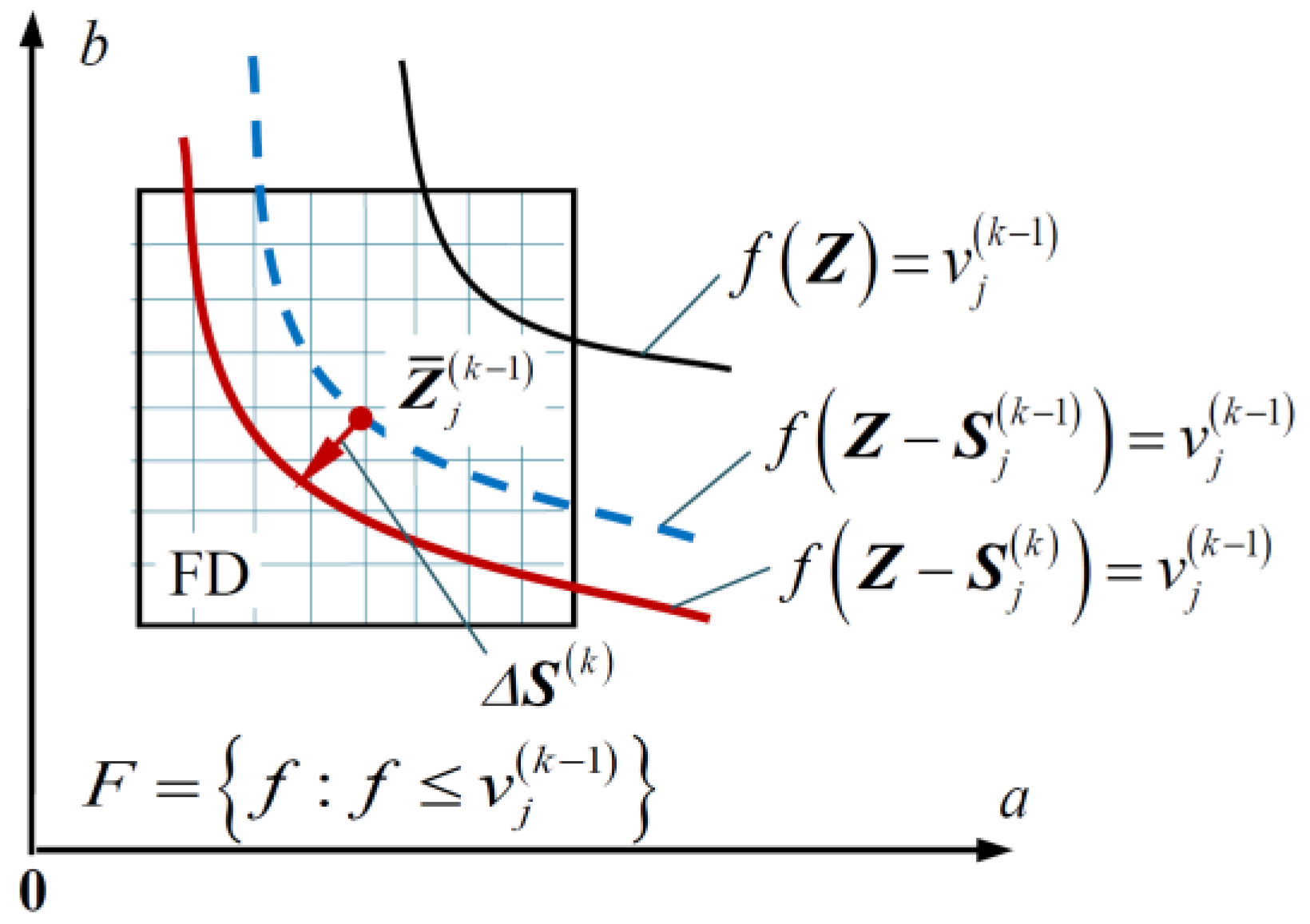
Figure 3.
The flowchart of the proposed method. EBRO: evidence-theory-based robust optimization; BPA: basic probability assignment.
Figure 3.
The flowchart of the proposed method. EBRO: evidence-theory-based robust optimization; BPA: basic probability assignment.

Figure 4.
A piezoelectric cantilever beam.
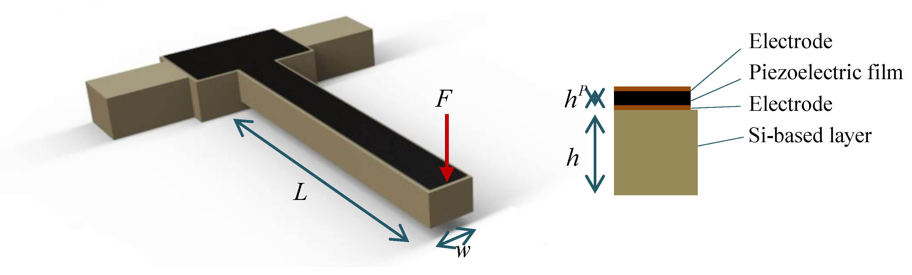
Figure 5.
Marginal BPAs of variables in the micro-force sensor problem. BPA: basic probability assignment; FD: frame of discernment.
Figure 5.
Marginal BPAs of variables in the micro-force sensor problem. BPA: basic probability assignment; FD: frame of discernment.
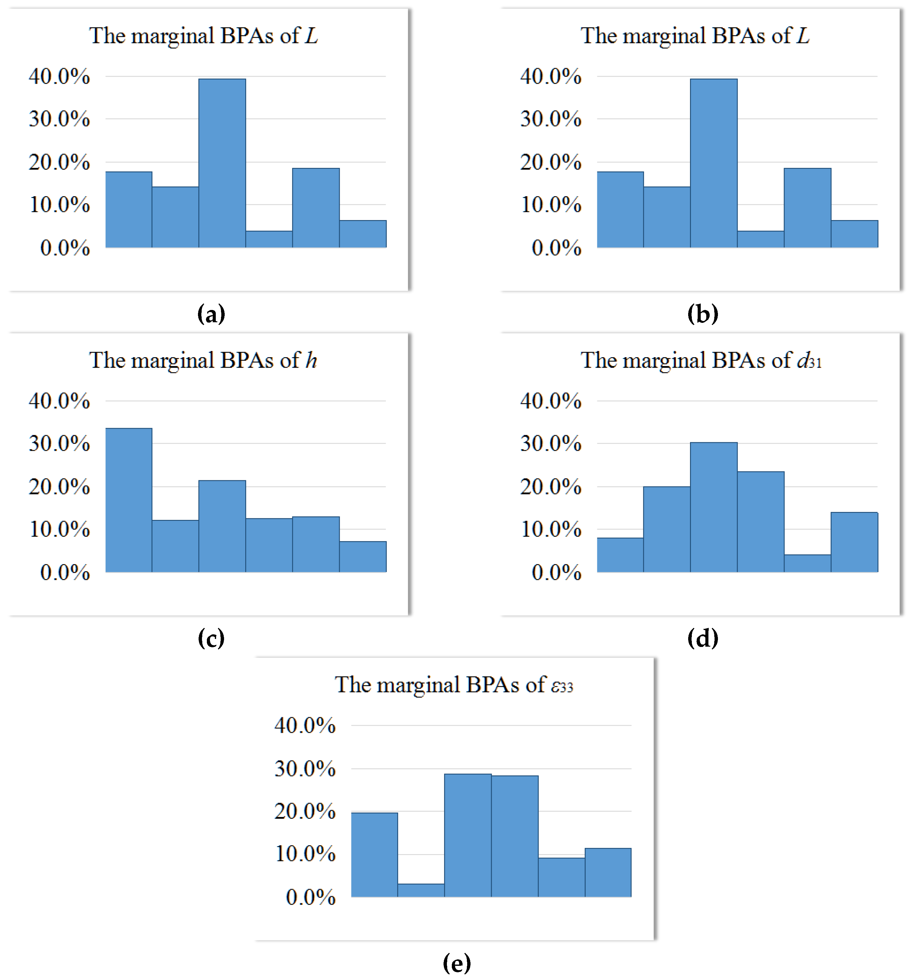
Figure 6.
The camera module (a) with an ultra-low-noise image sensor (b). PCB: printed circuit board.
Figure 6.
The camera module (a) with an ultra-low-noise image sensor (b). PCB: printed circuit board.
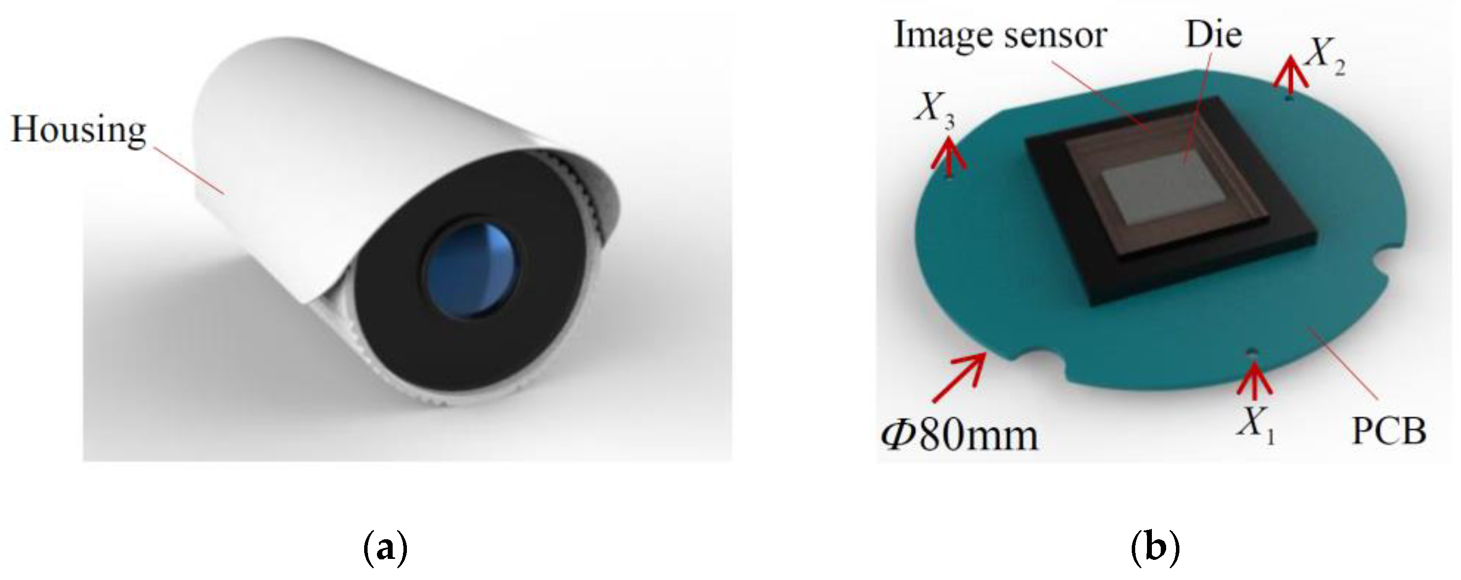
Figure 7.
The finite element model (FEM) of the image-sensor-mounted PCB. PCB: printed circuit board.
Figure 7.
The finite element model (FEM) of the image-sensor-mounted PCB. PCB: printed circuit board.
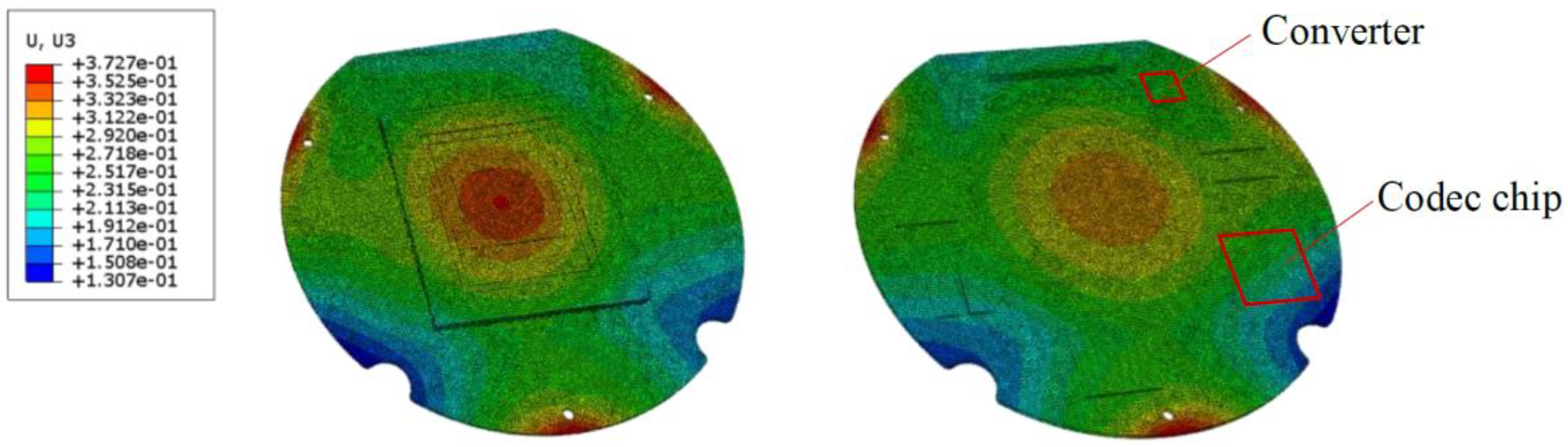
Figure 8.
The sensing structure of a capacitive accelerometer.
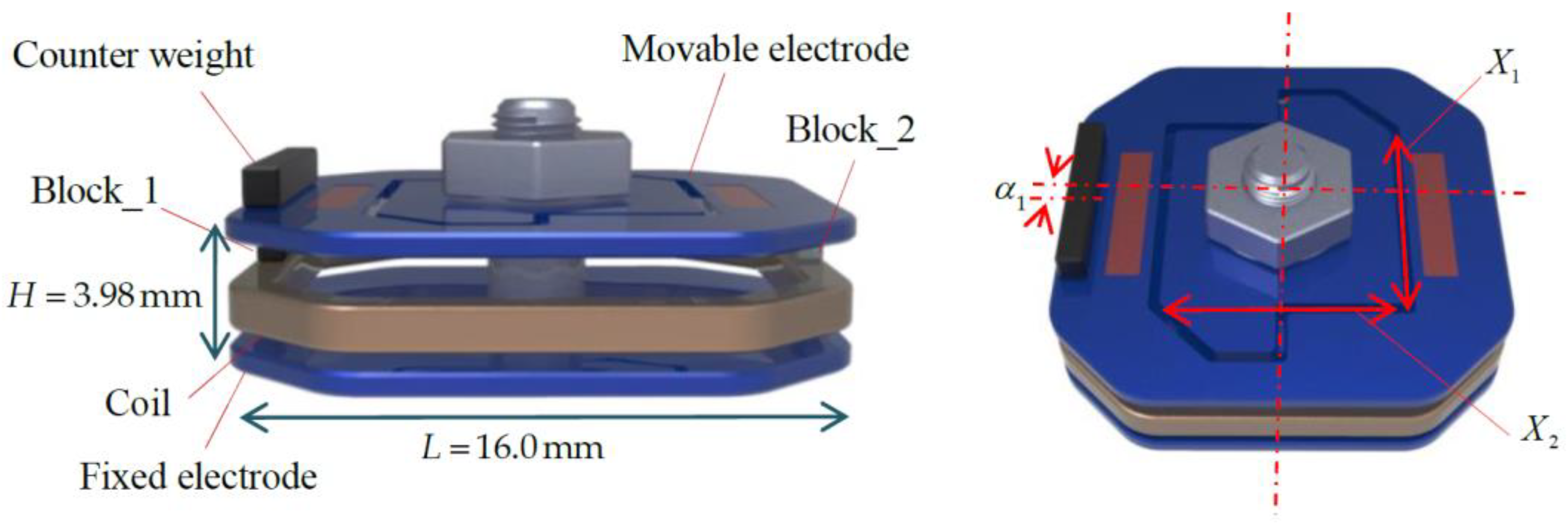
Figure 9.
The FEM of the capacitive accelerometer.

Figure 10.
The marginal BPAs of variables in the accelerometer problem. BPA: basic probability assignment; FD: frame of discernment.
Figure 10.
The marginal BPAs of variables in the accelerometer problem. BPA: basic probability assignment; FD: frame of discernment.

Table 1.
Optimal set of the micro-force sensor problem.
| Results | ||||||
| Proposed method | (mm) | 0.937, 0.086, 0.072 | 0.937, 0.086, 0.072 | 0.937, 0.086, 0.072 | 0.937, 0.086, 0.072 | 0.937, 0.086, 0.072 |
| 22.1 mV, 80.4% | 20.0 mV, 85.3% | 18.2 mV, 90.6% | 15.7 mV, 95.5% | 9.6 mV, 99.9% | ||
| Reference solution | 22.4 mV, 80.0% | 20.0 mV, 85.3% | 18.5 mV, 90.0% | 16.1 mV, 95.0% | 9.6 mV, 99.9% | |
Table 2.
The marginal BPA of variables in the image sensor problem.
| Xi, i = 1, 2, 3 (mm) | P1 (W) | P2 (W) | |||
|---|---|---|---|---|---|
| Subinterval | BPA | Subinterval | BPA | Subinterval | BPA |
| 6.7% | 37.5% | 6.5% | |||
| 24.2% | 17.6% | 23.8% | |||
| 38.3% | 5.4% | 32.2% | |||
| 24.2% | 19.1% | 12.5% | |||
| 6.7% | 20.4% | 24.9% | |||
Table 3.
The optimal set of the micro-force sensor problem.
| Results | Case 1:2 Dimensions | Case 2:3 Dimensions | Case 3:5 Dimensions | |
|---|---|---|---|---|
| Proposed method | 128 | 142 | 198 | |
| Iterations | 3 | 4 | 4 | |
| (mm) | (0.200, 0.185, 0.000) (0.200, 0.186, 0.000) (0.200, 0.188, 0.000) | (0.200, 0.185, 0.000) (0.200, 0.186, 0.000) (0.200, 0.187, 0.000) | (0.200, 0.187, 0.000) (0.200, 0.188, 0.000) (0.200, 0.190, 0.000) | |
| (1.35 μm, 85.1%) (1.70 μm, 96.5%) (2.00 μm, 100.0%) | (1.41 μm, 85.8%) (1.55 μm, 96.4%) (1.65 μm, 100.0%) | (1.74 μm, 86.4%) (2.06 μm, 96.1%) (2.62 μm, 100.0%) | ||
| Reference solution | (1.35 μm, 85.1%) (1.69 μm, 95.5%) (2.00 μm, 100.0%) | (1.41 μm, 85.8%) (1.55 μm, 96.4%) (1.65 μm, 100.0%) | (1.71 μm, 85.8%) (2.02 μm, 95.4%) (2.56 μm, 99.9%) | |
Table 4.
Material of accelerometer parts.
| Part | Fixed Electrode | Movable Electrode | Coil | Counter Weight | Block 1 | Block 2 |
|---|---|---|---|---|---|---|
| Material | Silicon | Silicon | Copper | Wolfram | Wolfram | Aluminium |
Table 5.
The optimal set of the accelerometer problem.
| Results | Proposed Method | Reference Solution |
|---|---|---|
| (mm) | (9.0661, 8.9042) (9.0659, 8.9040) (9.0657, 8.9038) (9.0653, 8.9035) (9.0653, 8.9035) (9.0653, 8.9035) | (9.0661, 8.9042) (9.0660, 8.9040) (9.0657, 8.9039) (9.0654, 8.9036) (9.0648, 8.9031) (9.0644, 8.9028) |
| (0.244 μm, 81.8%) (0.302 μm, 86.3%) (0.350 μm, 90.8%) (0.449 μm, 96.1%) (0.607 μm, 99.4%) (0.776 μm, 100.0%) | (0.244 μm, 81.8%) (0.279 μm, 85.2%) (0.338 μm, 90.1%) (0.424 μm, 95.5%) (0.594 μm, 99.2%) (0.733 μm, 99.9%) |
© 2019 by the authors. Licensee MDPI, Basel, Switzerland. This article is an open access article distributed under the terms and conditions of the Creative Commons Attribution (CC BY) license (http://creativecommons.org/licenses/by/4.0/).
Share and Cite
MDPI and ACS Style
Huang, Z.; Xu, J.; Yang, T.; Li, F.; Deng, S. Evidence-Theory-Based Robust Optimization and Its Application in Micro-Electromechanical Systems. Appl. Sci. 2019, 9, 1457. https://doi.org/10.3390/app9071457
AMA Style
Huang Z, Xu J, Yang T, Li F, Deng S. Evidence-Theory-Based Robust Optimization and Its Application in Micro-Electromechanical Systems. Applied Sciences. 2019; 9(7):1457. https://doi.org/10.3390/app9071457
Chicago/Turabian StyleHuang, Zhiliang, Jiaqi Xu, Tongguang Yang, Fangyi Li, and Shuguang Deng. 2019. "Evidence-Theory-Based Robust Optimization and Its Application in Micro-Electromechanical Systems" Applied Sciences 9, no. 7: 1457. https://doi.org/10.3390/app9071457
Note that from the first issue of 2016, this journal uses article numbers instead of page numbers. See further details here.