Supervised Machine-Learning Predictive Analytics for National Quality of Life Scoring

Featured Application

The method proposed in this paper is the first step towards predicting and scoring life satisfaction using a machine-learning model. Our method could help forecast the survival of future generations and, in particular, the nation, and can further aid individuals the immigration process.

Abstract

For many years there has been a focus on individual welfare and societal advancement. In addition to the economic system, diverse experiences and the habitats of people are crucial factors that contribute to the well-being and progress of the nation. The predictor of quality of life called the Better Life Index (BLI) visualizes and compares key elements—environment, jobs, health, civic engagement, governance, education, access to services, housing, community, and income—that contribute to well-being in different countries. This paper presents a supervised machine-learning analytical model that predicts the life satisfaction score of any specific country based on these given parameters. This work is a stacked generalization based on a novel approach that combines different machine-learning approaches to generate a meta-machine-learning model that further aids in maximizing prediction accuracy. The work utilized an Organization for Economic Cooperation and Development (OECD) regional statistics dataset with four years of data, from 2014 to 2017. The novel model achieved a high root mean squared error (RMSE) value of 0.3 with 10-fold cross-validation on the balanced class data. Compared to base models, the ensemble model based on the stacked generalization framework was a significantly better predictor of the life satisfaction of a nation. It is clear from the results that the ensemble model presents more precise and consistent predictions in comparison to the base learners.

1. Introduction

Since ancient times, individuals have been attempting to enhance themselves either for personal or for societal advantages. Recently there has been much debate surrounding the measuring of the quality of life of a society. Quality of life (QOL) reflects the relationship between individual desires and the subjective insight of accomplishments together with the chances offered to satisfy requirements [1]. It is associated with life satisfaction, well-being, and happiness in life. QOL demonstrates the general well-being of human beings and communities. It is shaped by factors such as income, jobs, health, and environment [2,3]. Well-being has a broad impact on human lives. Happy individuals have not only been found to be healthier and live longer but also to be significantly more productive and to flourish more [4,5]. Where we live affects our well-being and, consequently, we attempt to improve our locale. The places we live predict our future well-being. The social dimensions of quality of life (QOL) are strongly associated with social stability. Throughout the world individuals show interest in the happiness level of their nations and their position in global league tables. Different measures of provincial QOL present novel ways to find different arrangements that enable a society to reach a higher QOL for its citizens. It is deemed very important to know how each locale performs in terms of surroundings, education, security and all other points associated with prosperity. The social dimensions of QOL are strongly associated with social stability [6]. High well-being is not only vital for individuals themselves but also for the functionality of communities.

Thus, well-being is progressively argued to be an indicator of individual surroundings such as societies, foundations, organizations, and social relations. Estimating well-being enables us to identify and recognize the impacts of social change, within communities, on people’s life satisfaction and happiness and, consequently, serves as a measure for QOL. Recent studies of several organizations all over the globe demonstrated the association between the wealth and growth of a community, targeting sustainability and QOL [7]. These surveys have been performed at the state, country and international level, targeting the private sector, the common public, the scholarly community, the media, and individuals of both developed and developing nations. Research on regional well-being can help make policymakers aware of determinants of better living. The prediction of QOL visualizes and compares a number of key factors—housing, environment, income, education, jobs, health, civic engagement and governance, access to service, community and life satisfaction—that contribute to well-being in different countries.

The following quality of life indexes exist in the literature: the Happy Planet Index (HPI) [8], the World Happiness Index (WHI) [9], Gross National Happiness (GNH) [10], the Composite Global Well-Being Index (CGWBI) [11], Quality of Life (QL) [12], the Canadian Index of Wellbeing (CIW) [13], the index of well-being in the U.S. (IWBUS) [14], the Composite Quality of Life Index (CQL) [15] and the Organization for Economic Cooperation and Development (OECD) Better Life Index (BLI) [16]. Indictors of well-being are considered subjective issues while others are believed to be objective; this must be considered upon evaluation.

Table 1. Various dimensions of quality of life indicators.

	CQL	IWBUS	CIW	QL	CGWBI	GNH	WHI	HPI	BLI
Income (I)	√	√	√		√	√	√	√	√
Education (ED)	√	√	√	√	√	√			√
Health (H)	√	√	√	√	√	√	√	√	√
Environment (E)			√	√	√	√	√	√	√
Housing (H)	√			√	√				√
Time use (T)	√		√			√			√
Jobs (J)	√			√	√				√
Community (C)			√		√	√	√		√
Governance (G)	√		√	√		√			√
Generosity (G)							√
State of IQ		√
Safety (S)	√	√		√	√				√
Choices freedom (C)		√				√	√
Life Satisfaction (L)	√	√	√		√	√	√	√	√
No. of Dimensions	9	7	8	7	9	9	7	4	11

depicts both objective and subjective dimensions of different indicators that contribute to the measure of well-being of a country. Of all the indicators of well-being, the OECD Better Life Index is one of the most accepted initiatives evaluating quality of life.

The OECD framework indicates the country’s efforts toward living satisfaction and public happiness. This framework considers life satisfaction to be multifaceted, built with material (jobs and earnings, income and wealth, and housing conditions) and nonmaterial components (work-life balance, education and skills, health status, civic engagement, social connections, environmental quality, governance subjective well-being, and personal security). Moreover, the system stresses the significance of evaluating the major assets that steer well-being over time, which should be cautiously supervised and administered to attain viable well-being. The resources can be evaluated through natural, social, human, and economic capital [16].

The OECD Better Life Index (BLI) consists of 11 subjects—jobs (J), housing (H), income (I), education (ED), community (C), governance (G), health (H), environment (E), safety (S), life satisfaction (L), work-life balance (W)—that are recognized as significant, in terms of of quality of lifestyles and material living conditions, for examining well-being throughout different countries [17]. The index is a combined index that cumulates a country’s well-being conclusions using the weights stated by online end users. It envisages and weighs against some of the key features—housing, education, environment—that add to well-being in OECD countries. Using averaging and normalization, 20 sub-indicators were added to these main indicators. By selecting a weight for each sub-indicator, a user can rank countries according to their weighted sum. Figure 1 depicts the user rating of different well-being dimensions of 743,761 BLI users living within the OECD area [18]. The ratings concluded that all dimensions of quality of life are generally considered to be significant; nevertheless, education, health and life satisfaction dimensions are ranked higher. The lower ranked dimensions include community and civic engagement.

Recent studies of several organizations throughout the world demonstrate the connection between prosperity and growth of societies, targeting sustainability and QOL. A place with high-quality living has more jobs opportunities. Natives are not willing to spend in places where there is not a good quality of life. The present study was the first step towards predicting life satisfaction scores using a machine-learning model. It could affect the survival of future generations and further aid the immigration process. The goal of the study was to predict the life satisfaction score of a country based on various key factors contributing to quality of life using machine-learning stack-based ensemble models.

There are different techniques to evaluate nationwide happiness and subjective well-being. One such approach is via predictive analytics that consider the dataset and make predictions based on past events or modeling. The current work proposes a supervised two-tier stack-based analytical model for predicting the life satisfaction score of a country based on the OECD dataset. The work presents a cost-effective method of life satisfaction prediction with a high degree of efficiency.

1.1. Research Contribution

The major contributions of this paper are as follows:

• This paper presents an ensemble predictive analytic model that combines the various qualities of individual prediction models for better prediction and more consistent results.
  From a computational point of view, the ensemble approach is more in demand and performed notably better than the best performing support vector regressor (SVR) base models.
• The superiority of the novel ensemble prediction model was validated with BLI data from OECD regional statistics.
• The proposed ensemble prediction demonstrated its dominance in comparison to classic base models, and the predictive strength of the developed ensemble model revealed its superior life satisfaction prediction compared to the classical models.

Explorations of the importance of the proposed prediction model, the contrast with classical models, and the verification of the prediction efficiency of the proposed model were carried out.

1.2. Organization

The paper is organized as follows: Section 2 reflects on the related works; Section 3 consists of the details and theoretical background of the proposed analytical model; Section 4 sums up the results of the proposed model against various performance metrics, and Section 5 presents the conclusion and future scope of this research.

2. Related Works

To date, little research has been performed pertaining to the clarification of perceptions of well-being in machine-learning models. In spite of the fact that the significance of machine-learning for the study of high dimensional, non-linear data is on the rise, the numerical issues in sociology are hardly ever examined in terms of machine-learning. The following text mirrors some research directions of applications of machine-learning within the social sciences, especially in regards to personality.

The authors Durahim and Coşkun [19] targeted the Middle Eastern country of Turkey, finding its gross national happiness (GNH) via a sentiment analysis model. The work utilized 35 million tweets to train the model. The results were an average of 47.4% happy (positive), 24.2% unhappy (negative), and 28.4% neither happy nor unhappy (neutral), for the first half of the year 2014. The authors further stated that users’ happiness levels strong correlated with Twitter characteristics. Jianshu, et al. [20] proposed, as a way to predict the happiness score of a group in a photograph in a normal setting, using deep residual nets. The method combines the facial scene features in a sequential manner by mining Long Short Term Memory (LSTM) and deep face attribute illustrations. The solution employs both ordinal and linear regression. The proposed method gave better results than the baseline model in terms of both validation and test set. Takashi and Melanie Swan [21] studied the contribution of personal genome informatics and machine-learning to understandings of well-being and happiness sciences. The authors concluded that happiness is best formulated as a ‘big data problem”. The authors of Reference [22] proposed a technique for measuring job satisfaction using a decision support system based on the multi-criteria satisfaction analysis (MUSA) technique and the genetic algorithm. In this technique the authors combined a genetic algorithm with the MUSA technique to acquire a robust reduction of fitness value. Yang and Srinivasan [23] described life satisfaction as a component of subjective well-being. Their work scored life satisfaction by examining two years of Twitter data by applying techniques to find both dissatisfaction and satisfaction with life. Authors Kern et al. [24] developed models of well-being based on natural language. The models were built through group-sourced ratings of tweets and Facebook bulletins, creating a text-based predictive model for different aspects of well-being.

The majority of the literature has focused on sentimental analysis for prediction of QOL. No work has been done so far using income, jobs, health, education, environmental outcomes, safety and housing, and community as life satisfaction features predictive of QOL. Machine-learning is still seldom applied to social problems like the present well-being prediction. Nevertheless, machine-learning guarantees, for example, the identification of the basic structures deciding prosperity. It acts intelligently to make predictions and identify patterns from given data. Consequently, this study applied a wide range of different machine-learning algorithms to identify various features affecting the life index score of any country and to test the capabilities of machine-learning approaches for the prediction of well-being. The proposed approach focused on using machine-learning algorithms to predict a country’s quality of life by forecasting the score of the country using two-tier stack-based ensemble models.

3. Materials and Methods

In this section, we will discuss the proposed methodology, in detail, along with a description of the classification algorithms used. Figure 1 presents the prediction process of the stacked generalization framework. Figure 2 shows the workflow of the proposed work. The dataset used in this paper is described in Section 3.1. In Section 3.2, a detailed theoretical background of the proposed model is presented. Finally, the classification approaches used are discussed in Section 3.3.

3.1. Dataset

The dataset was taken from the OECD regional statistics of the BLI of different countries, representative of the last four years [25]. The dataset consists of four different .csv files, one per year from 2014 to 2017, having a total of 38 instances, 11 major attributes, 23 sub-attributes and no missing values in any file. The dataset is a record of 38 countries. The .csv files contain 3390, 3292, 3538 and 3398 instances for 2014 to 2017 data respectively.

Table 2. Features subset.

Features	Subsets
Housing	Dwellings without basic facilities (H1), rooms per person (H2), housing expenditure (H3)
Jobs	Labor market insecurity (J1), employment rate (J2), long-term unemployment rate (J3), personal earnings (J4)
Income	Household net adjusted disposable income (I1), household net financial wealth (I1)
Community	Quality of support network (C1)
Income	Household net adjusted disposable income (I1), household net financial
Environment	Air pollution (E1), water quality (E2)
Education	Educational attainment (ED1), student skills (ED2), years educated (ED3)
Civic engagement	Stakeholder engagement for developing regulations (CI1), voter turnout (CI2)
Life satisfaction	As a target (L1)
Health	Life expectancy (HE1), self-reported health (HE2)
Work-life balance	Employees working very long hours (W1), time devoted to leisure and personal care (W2)
Safety	Feeling safe walking alone at night (S1), hHomicide rate (S2)

gives the contribution of each attribute in terms of measuring life satisfaction.

The major attributes are namely: education, housing, community, environment, income, civic engagement, government jobs, and health.

Table 3. Attribute descriptions.

Attribute Name	Description
Income	Income is an important component for individual well-being. It is also associated with life satisfaction, allowing people to satisfy their basic life needs.
Jobs	Jobs, or employment, represents another factor of well-being and has a huge impact on people’s situations. Having a job facilitates the expansion of abilities, and affects elements of well-being related to social connections, health, and life satisfaction.
Health	There are, likewise, local variations in well-being results, which are incompletely disclosed due unequal access to health and well-being administrations.
Education	Education can have numerous private returns, in terms of skills, work, and well-being. In addition, there is evidence that education has imperative social returns, which have an impact on the overall productivity, incremental political cooperation and crime rates of a place.
Environmental Outcomes	The condition of a neighborhood affects prosperity. Currently, air contamination is incorporated but further ecological quality factors ought to be incorporated, for example, water and waste.
Safety	Individual security is the degree to which individuals feel sheltered and protected from individual mischief or wrongdoing.
Civic engagement and Governance	Institutional conditions and administration matter for singular prosperity, remembering that a considerable amount of the approaches that have direct influence on individuals’ lives are established at this level. Voter turnout indicates the status of open belief in administration and of subjects’ support in the constitutional procedure.
Access to services	Availability of administrations is also one of the key measurements of prosperity, influencing how individuals get what is important to fulfil their needs.
Housing	In measuring well-being, housing is an important factor. Shelter is one of the most basic human needs, along with food and water.
Community	Good relations, social network supports and trust in others are considered important sources of individual well-being.
Life Satisfaction	This measures how people experience and evaluate their lives.

depicts the sub-features within each major attribute. These sub-features were selected based on statistic principles, such as data quality and relevance, and are in discussion with OECD associated nations. These sub-features act as a measure of well-being, especially inside the context of a country-comparative exercise.

3.2. Proposed Methodology

The process employed a 10-fold cross-validation that served as the outer most loop in training the model. The whole dataset was split into 10 sets. For every set, recursive feature elimination was performed on the training set, to extract the optimal set of features. Recursive feature elimination involves the repeated construction of a model, selecting and discarding the worst performing features and then reiterating the whole process with the remaining features. This process was exercised until th all features in the dataset were exhausted. Base models are trained using the final selected features of a training dataset. This generates a feature selection mask that is further applied to the test set. The refined test set was fitted on the model. Figure 2 depicts the methodology of the proposed scheme for efficient QOL prediction. The whole process was repeated for all 10 folds for the seven base models. The performance of the models was evaluated using Pearson Correlation coefficient (r), Coefficient (R), root mean squared error (RMSE) and accuracy parameters. The four topmost base models were selected, on the basis of RMSE, and further utilized for stacking generalization.

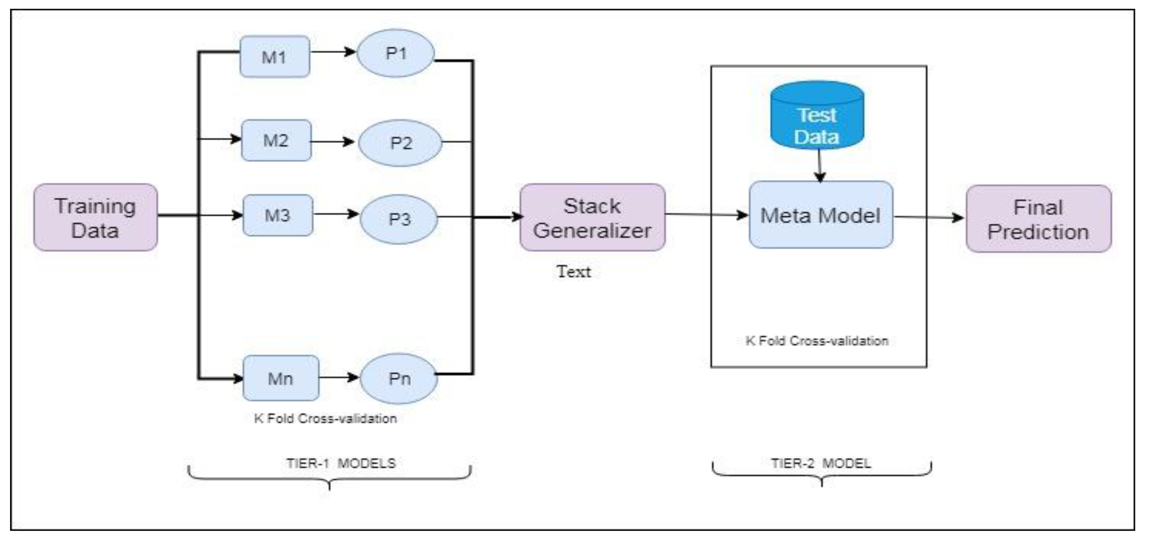
The stacked generalization framework incorporates two kinds of models: (i) Tier 1 models (seven base models) and (ii) a Tier 2 model, i.e., one meta-model. The top four base models were selected based on their RMSE value. The stacked generalization exploited the Tier 2 approach to train from the outcomes of the Tier 1 approaches, i.e., the top base classifiers were combined by a meta-level (Tier 2) classifier to predict the correct class based on the predictions of the top base level (Tier 1) classifiers. Usually, the framework of stacked generalization achieves more accurate predictions than the best Tier 1 model.

The technique generated the proposed model in two phases:

Phase 1—Seven different models were trained for life satisfaction score prediction. (Tier 1 models)

Phase 2—The top four models (based on RMSE) were combined in a group of three, making four different combinations to further improve the performance of the prediction model (Tier 2 model).

The final output was selected using the stacking technique [26].

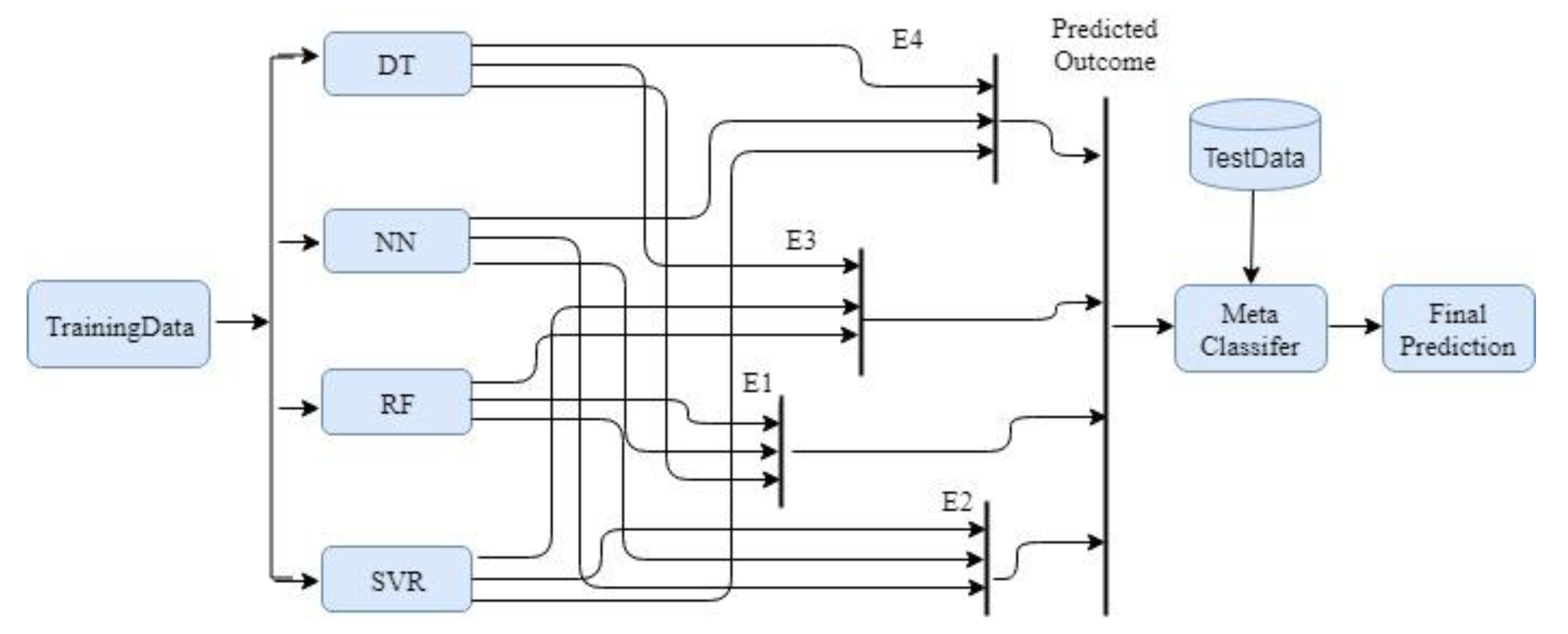
The flow of the proposed methodology is presented in Figure 3. The figure depicts the schematic diagram of the final combination of all top four ensemble models. In this work, a combination of three machine-learning models was used to develop an ensemble machine-learning approach for determining the life satisfaction score of a country. Each top base learner was trained using 10-fold cross-validation, wherein the training set was split into 10 folds. A base model was fitted on the 9 parts and predictions were made on the 10th part. This process was repeated 10 times for each fold of training data. The base model was then fitted on the overall training dataset to calculate its performance on the test set. The previously mentioned steps were applied to all the base learners. At this time, the output labels (predicted) (i.e., the predictions from the training set) of the first-level classifiers were used as new features for the second level learner, and the original labels were utilized as labels inside the new dataset. The second level model was used to make predictions on the test set. As the data traveled through the three models, the models trained the data to offer reliable and precise outcomes. The best ensemble model was based on RMSE contributes to the final prediction.

3.3. Models Used

This section gives brief descriptions of the various machine-learning models that were used in predicting the life satisfaction score. Each model was coded in R and calculated various regression parameters to find the best model.

A decision tree was used to build a regression and classification model, as a tree-like graph. It focused on an easily understandable representation form and was one of the most common learning methods. It can be easily visualized in the tree structure format. A decision tree is built by iteratively splitting the dataset on the attribute that separates the data into different existing classes until a certain stop criterion is reached [27]. The result was in the form of a tree with leaf nodes and decision nodes. It was structured like a flow-chart; each inner node was signified by a rectangle and each leaf node by an oval.

A neural network (NN) is a supervised machine algorithm. The goal of the algorithm is to assign each input to one of the many predefined output classes based on a prediction value. The processing in a neural network occurs when an input value passes through a series of batches of activation units [28,29]. These batches are called layers. A layer of activation units uses the output values of the previous layer and input and processes them simultaneously to generate outputs that are passed on to the next layer. This process continues until the last layer generates the final cumulative predictions.

A random forest (RF) is also a machine-learning model used for predictive analytics. This is an ensemble learning method that creates numerous regression trees and aggregates their results. It trains every tree independently using a random sample of the data [30,31]. This randomness makes the model more powerful. The main advantages of the model are its capacity to generalize, its low sensitivity to parameter values and its built-in cross-validation. The random forest model is excellent at managing tabular records with numerical functions or categorical functions.

The SVR is a machine-learning model can be applied to both classification and regression problems. Support vector machines have been effectively utilized to tackle nonlinear regression and time arrangement issues. The SVR maps, nonlinearly, the original information into a higher dimensional component space [32]. While fabricating the model, it makes use of the mathematical function to expand the dimensions of the sample until the point where it can directly isolate the classes in the test set. The mathematical function that expands the dimension is called a kernel function. This function changes the data in such a manner that there is more probability of separable classes. To find the optimal separation, it can linearly isolate the classes.

Cubist regression modeling uses rules with added instance-based corrections [33]. It is an adjunct of Quinlan’s M5 model tree. In this model, linear regression models act as leaf nodes in the grown tree along with intermediate linear models at every stage of the tree. The leaf node of the tree representing the linear regression model makes a prediction that is “smoothed” using the forecast from the linear model in the earlier node of the tree. The tree is condensed into a group of rules. The rules are eradicated via pruning and/or united for generalization.

A generalized linear model (GLM) is an adjunct of a general linear model to families of outcomes that are not normally distributed but have probability density functions related to the normal distribution (called the exponential family). The generalized linear model includes a link method that links the average of the response to the linear grouping of the predictors of the model, function, inverse function etc. [34]. Here, the least square technique is used to calculate the tuning parameters of the model.

An elastic net combines L1 norms (lasso) and L2 norms (ridge regression) into a penalized model for generalized linear regression [35]. This gives it sparsity (L1) and robustness (L2) properties. Regularization is used to avoid overfitting the model to the training data. Lasso (L1) and ridge (L2) are the commonly used regularization techniques. Ridge regression does not zero out coefficients, it penalizes the square of the coefficient. In lasso, some of the coefficients can be zero, meaning that it does variable selection as well. Lasso penalizes coefficients, unlike ridge which penalizes squares of coefficients. Ridge and lasso are combined in the hybrid regularization technique called elastic net.

4. Experimental Results

On a standalone machine, ten different models were implemented in R programming [36] using an Intel Core^®i5 processor at 2.80 GHz and 4.00 GB RAM, running on a 64-bit operating system. The steps can be divided into five main stages:

• 10-fold cross-validation with feature selection;
• Prediction using seven machine-learning algorithms;
• Selection of the top four learners based on RMSE;
• Employment of stacking ensemble on these learners (using three at a time in combination) and selection of the best ensemble approach.

The dataset contained no missing values. The values within the dataset were present on a mixed scale, in the form of ratios, percentage and average scores. The data was normalized using the min.max() normalization function in R. We used a realistic dataset so we did not have to consider outliers of the dataset and simulated our work using the original dataset [25].

To optimize the performance, the parameters of the models needed to be tuned.

Table 4. Models with tuning parameters.

Model	Method	Libraries	Tuning Parameters
Cubist	cubist()	cubist	neighbors = 30, Committees = 10
Decision tree	rpart()	rpart	minsplit = 20, minbucket =7, maxdepth = 30
Elasticnet	enet()	elasticnet	fraction, lambda = 0.05
Linear model	lm()	glm	None
Neural network	nnet()	nnet	maxit = 100, hlayers = 10, MaxNWts = 1000
Random forest	rf()	randomForest	mtry = 3, importance = TRUE
Support vector machine	svm()	e1071	nu = 10, epsilon = 0.5

shows the models used in the present study along with their tuning parameters and required packages. The work utilizes the rfe() and rfeControl() functions for feature selection with cross-validation.

Table 5. Features selected for data of different years.

Year	Selected Set of Features
2014	L1≈ f (H1, I1, J2, J3, E2, HE2)
2015	L1≈ f (H2, J2, J3, CI2, HE1, HE2)
2016	L1≈ f (H1, H3, J1, J2, J3, J4, C1, ED1, ED3, E1, E2, CI1, CI2, HE2, S1, W1)
2017	L1≈ f (H3, J1, J2, J3, J4, C1, ED3, E1, E2, CI2, HE2)

lists the features selected for different years. The results from the various models and their ensembles were examined and compared with each other on the basis of several evaluation criteria. The following text gives the brief description of the evaluation parameters applied to the regression models.

A correlation coefficient (r) is also called a linear correlation. It quantifies the strength of the relationship among dependent and independent variables. The linear correlation is also referred to as Pearson’s correlation or product moment correlation. The estimation of r lies between −1 and 1. If the value of r is in the negative range then it is a weak relationship. If it is in the positive range then it indicates a strong relationship. It is represented as in Equation (1):

$$r=\frac{{{\displaystyle \sum }}^{ }xy-\frac{{{\displaystyle \sum }}^{ }x{{\displaystyle \sum }}^{ }y}{n}}{\sqrt{({{\displaystyle \sum }}^{ }{x}^2-\frac{{({{\displaystyle \sum }}^{ }x)}^2}{n})-({{\displaystyle \sum }}^{ }{y}^2-\frac{{({{\displaystyle \sum }}^{ }y)}^2}{n})}}.$$

(1)

The coefficient of determination (R) is a statistical evaluation of how well the relapse line approximates the actual record points. The estimation of R extends between 0 and 1 and denotes the strength of linear association between x and y. It is calculated as given in Equation (2):

$$R=r^2.$$

(2)

The root mean squared error (RMSE) proposes the complete match of the model to the data—how close the actual data values are to the predicted values. RMSE is a measure of how appropriately the model predicts the response. It is regularly utilized to calculate the dissimilarity of values estimated by a model and the actual value. RMSE is computed as in Equation (3):

$$\mathrm{RMSE}=\sqrt{{{\displaystyle \sum }}_{i=1}^n\frac{{\left(\mathrm{Actual}-\mathrm{Predicted}\right)}^2}{n}}.$$

(3)

Accuracy is calculated as percent variation of a predicted value, with actual values up to an acceptable limit of error. This is given in Equation (4), where, p_i is the ith predicted target, ai is the ith original value, err is the acceptable error and n is the total count of samples.

$$\begin{gathered} \mathrm{Accuracy}=\frac{100}{n}{{\displaystyle \sum }}_{i=1}^n{d}_i, \\ {d}_i=\{\begin{array}{c}1 if abs\left(p_i-a_i\right)\le \mathrm{err}\\ 0 \mathrm{other} \mathrm{wise} \end{array} \end{gathered}$$

(4)

Total time refers to the time it takes the entire program to execute the model, compute the different parameters of the regression data, and evaluate the outcome.

Table 6. Average results of base models.

Year	Models Used	r	R	RMSE	Accuracy	Total Time
2014	Cubist	0.77	0.60	0.8	73.92	32.42
	Decision tree	0.24	0.06	0.537	81.66	30.49
	Elastic net	0.57	0.35	0.816	70.88	45.79
	Linear model	0.84	0.71	0.748	77.93	33.72
	Neural network	0.73	0.54	0.48	84.99	31.35
	Random forest	0.84	0.71	0.507	83.22	30.77
	Support vector regressor	0.79	0.62	0.371	90.00	30.66
2015	Cubist	0.76	0.61	0.832	72.96	35.22
	Decision tree	0.36	0.13	0.763	81.66	34.91
	Elastic net	0.57	0.34	0.850	70.50	43.50
	Linear model	0.81	0.65	0.803	77.59	38.75
	Neural network	0.69	0.49	0.594	83.33	28.77
	Random forest	0.83	0.71	0.408	86.47	31.00
	Support vector regressor	0.83	0.69	0.352	88.33	30.43
2016	Cubist	0.62	0.39	0.869	77.33	32.12
	Decision Tree	0.54	0.35	0.614	83.32	32.67
	Elastic net	0.73	0.54	0.867	77.55	45.86
	Linear Model	0.69	0.48	0.808	78.79	40.14
	Neural Network	0.78	0.63	0.464	85.00	33.52
	Random Forest	0.82	0.68	0.406	86.66	33.14
	Support vector regressor	0.81	0.66	0.322	90.00	28.95
2017	Cubist	0.63	0.40	0.843	77.97	35.45
	Decision tree	0.68	0.48	0.44	88.26	32.89
	Elastic net	0.71	0.52	0.879	77.84	43.98
	Linear model	0.69	0.48	0.727	79.33	40.14
	Neural network	0.78	0.61	0.463	83.33	36.20
	Random forest	0.82	0.67	0.45	86.67	37.02
	Support vector regressor	0.81	0.66	0.378	91.58	30.09

depicts the average results of various performance metrics obtained from the seven different machine-learning models. The top models were selected based on RMSE parameters. The parameters measured the quality of prediction. The lower values of RMSE indicated better fit models. From the results of the year 2014, it was clear that the SVR model achieved the lowest RMSE value, 0.37, with the highest accuracy, 90%, compared to the rest of the algorithms. The model’s elastic net was found to be the worst performer, with an RMSE value of 0.81 and accuracy of 70.9%. The case for the years 2015 to 2017 were similar. The SVR model gave the best results, in terms of RMSE value, 0.35, 0.32, and 0.38 for 2015, 2016 and 2017, respectively. Also, the accuracy, using the SVR model, was, on average, above 90%. The RMSE value for the cubist, elastic net and linear models was higher than 0.80 for the year 2015. For the year 2016, both elastic net and cubist give a lower RMSE value, 0.87, whereas random forest and neural networks had RMSE values near 0.40. SVR had the lowest RMSE value, 0.32. Furthermore, the same model was able to be exceedingly specific in predicting life satisfaction from the dataset, with an RMSE of 0.38 and accuracy of 91.58%, for the year 2017.

The performance assessment of all the models considered was graphically envisioned with a sketching boxplot [37]. It portrayed the empirical distribution of the data. Figure 4a–d represents the boxplot for the base models. In the plot, the x-axis represents the model names and the y-axis labels the RMSE parameter. It is clear from the boxplots that the SVR gave improved and consistent results compared to the other models, in terms of the RMSE metric for each year. The absence of outliers also added to the steadiness of the models. The boxplot depicts RF and NN to be the second-best performers, of all the years, in terms of RMSE.

As each category of the model has potential and shortcomings, consequently, the top models (based on RMSE) were combined to generate ensemble models. Ensembles use a number of different algorithms in order to achieve superior predictive performance than could be achieved by using any of the individual learners [38]. Based on the results, the top four models, namely decision tree (DT), support vector regressor (SVR), neural network (NN), and random forest (RF), were selected for the development of the ensemble models and three models (out of these four models) were combined in each ensemble. The following are the top four ensemble models chosen based on the values of RMSE.

• E1—(DT, NN, RF)
• E2—(NN, RF, SVR)
• E3—(DT, RF, SVR)

All models were combined in the three groups (making four different combinations) to improve the performance of the models using the stacking technique.

Table 7. Results of ensemble models.

Year	Models	r	R	RMSE	Accuracy (%)	Total Time
2014	DT, NN, RF	0.74	0.55	0. 450	85.24	30.25
	NN, RF, SVR	0.95	0.91	0.394	91.56	40.13
	DT, NN, SVR	0.68	0.46	0.478	85.00	40.70
	DT, RF, SVR	0.78	0.61	0.342	94.50	30.29
2015	DT, NN, RF	0.79	0.62	0.417	88.41	31.43
	NN, RF, SVR	0.90	0.81	0.402	90.00	42.32
	DT, NN, SVR	0.87	0.76	0.453	88.00	39.16
	DT, RF, SVR	0.94	0.87	0.306	93.00	29.16
2016	DT, NN, RF	0.75	0.56	0.438	86.44	33.14
	NN, RF, SVR	0.82	0.66	0.442	89.23	39.50
	DT, NN, SVR	0.71	0.50	0.437	89.23	37.43
	DT, RF, SVR	0.73	0.53	0.329	92.43	32.44
2017	DT, NN, RF	0.80	0.64	0.401	90.00	32.76
	NN, RF, SVR	0.83	0.68	0.386	92.54	40.29
	DT, NN, SVR	0.94	0.88	0.378	90.00	40.02
	DT, RF, SVR	0.82	0.67	0.292	96.42	30.22

shows the performance parameter values obtained from the four ensembles after the application of the stacking scheme on the three prediction results. The table depicts the combination of the DT, RF and SVR models and gives the best results in terms of RMSE compared to the rest of the ensembles for each year. Moreover, the ensemble combining DT, NN and SVR gave the highest RMSE value for the year 2014 and 2015. Both the ensemble with DT, NN, and SVR and that with DT, NN, and RF obtained the highest RMSEs, 0.43, for the year 2016. The ensemble DT, NN, and RF gave the worst RMSE value, 0.40, for the year 2017.

Figure 5 shows the comparative analysis of ensemble models in terms of average RMSE. The ensemble model (combining DT, RF, and SVR) gave the lowest RMSE values, i.e., 0.34, 0.30, 0.32 and 0.29 for each year from 2014 to 2017 respectively, in the prediction of countrywide life satisfaction. The proposed approach was a multilevel ensemble model, a group of three base models that outperformed the top performing SVR model. The results revealed that the ensemble model had better accuracy compared to the base model accuracy.

5. Conclusions and Future Work

In the current work, a supervised two-tier ensemble approach for predicting a country’s BLI score was proposed. The work presented a cost-effective method of BLI prediction with a high degree of efficiency. The dataset consisted of four different files for 2014 to 2017. The capability of the model to predict life satisfaction relied on the proper training features, chosen using a recursive elimination method with 10-fold cross-validation. The work combined three of the top four models, with simple averaging, to enhance the performance of the regression. The model was built using an ensemble approach and was evaluated using r, R, RMSE, and accuracy performance evaluators. The empirical relevance of diversity estimates were assessed with regard to combining the regression models by stacking. The model was about 90% accurate for predicting the life satisfaction score of a country. The present study was the first step towards forecasting the BLI score using machine learning based regression model that can influence the survival of future generations and further aid the immigration process. The work can be extended by tuning the parameters of the base models using meta-heuristic approaches to improve the prediction accuracy.

References

- Estoque, R.C.; Togawa, T.; Ooba, M.; Gomi, K.; Nakamura, S.; Hijioka, Y.; Kameyama, Y. A review of quality of life (QOL) assessments and indicators: Towards a “QOL-Climate” assessment framework. Ambio 2018, 1–20. [Google Scholar] [CrossRef] [PubMed]
- Stone, A.A.; Krueger, A.B. Understanding subjective well-being. In For Good Measure: Advancing Research on Well-Being Metrics Beyond GDP; Stiglitz, J.E., Fitoussi, J.-P., Durand, M., Eds.; OECD: Paris, France, 2018; 163p. [Google Scholar]
- World Health Organization. Social Determinants of Health. How Social and Economic Factors Affect Health. Available online: http://publichealth.lacounty.gov/epi/docs/SocialD_Final_Web.pdf (accessed on 2 January 2019).
- Moore, S.M.; Diener, E.; Tan, K. Using multiple methods to more fully understand causal relations: Positive affect enhances social relationships. In Handbook of Well-Being Diener; Oishi, S., Tay, L., Eds.; DEF Publishers: Salt Lake City, UT, USA, 2018. [Google Scholar]
- Michalos, A.C. Education, happiness and wellbeing. In Connecting the Quality of Life Theory to Health, Well-Being and Education; Springer: Cham, Switzerland, 2017; pp. 277–299. [Google Scholar]
- Lamu, A.N.; Olsen, J.A. The relative importance of health, income and social relations for subjective well-being: An integrative analysis. Soc. Sci. Med. 2016, 152, 176–185. [Google Scholar] [CrossRef] [PubMed]
- Bakar, A.A.; Osman, M.M.; Bachok, S.; Ibrahim, M.; Mohamed, M.Z. Modelling economic wellbeing and social wellbeing for sustainability: A theoretical concept. Procedia Environ. Sci. 2015, 28, 286–296. [Google Scholar] [CrossRef]
- Index, H.P. About the Happy Planet Index. Repéré sur le Site de HPI, Section About the HPI. 2016. Available online: http://www.happyplanetindex.org/http://www.happyplanetindex.org/about (accessed on 10 January 2019).
- Country Economy. Available online: https://countryeconomy.com/demography/world-happiness-index (accessed on 8 January 2019).
- Ritu, V. Gross national happiness: Meaning, measure and degrowth in a living development alternative. J. Political Ecol. 2017, 24, 476–490. [Google Scholar]
- Jad, C.; Irani, A.; Khoury, A. The composite global well-being index (CGWBI): A new multi-dimensional measure of human development. Soc. Indic. Res. 2016, 129, 465–487. [Google Scholar]
- Somarriba, N.; Pena, B. Synthetic indicators of quality of life in Europe. Soc. Indic. Res. 2009, 94, 115–133. [Google Scholar] [CrossRef]
- Graham, A. Assessing the Environment Domain of the Canadian Index of Wellbeing: Potentials for Leveraging Policy. Master’s Thesis, University of Waterloo, Waterloo, ON, Canada, 2015. [Google Scholar]
- Pesta, B.J.; Mcdaniel, M.A.; Bertsch, S. Toward an index of well-being for the fifty U.S. States. Intelligence 2010, 38, 160–168. [Google Scholar] [CrossRef]
- Greyling, T. A Composite Index of Quality of Life for the Gauteng City-Region: A Principal Component Analysis Approach. Wits Institutional Repository on DSpace 2015. Available online: http://hdl.handle.net/10539/17365 (accessed on 12 January 2019).
- Balestra, C.; Boarini, R.; Tosetto, E. What matters most to people? Evidence from the OECD better life index users’ responses. Soc. Indic. Res. 2018, 136, 907–930. [Google Scholar] [CrossRef]
- Sirgy, M.; Estes, J.R.J.; Selian, A.N. How we measure well-being: The data behind the history of well-being. In The Pursuit of Human Well-Being; Springer: Cham, Switzerland, 2017; pp. 135–157. [Google Scholar]
- Organisation for Economic Co-operation and Development. How’s Life? Measuring Well-Being; OECD: Paris, France, 2015. [Google Scholar]
- Durahim, A.O.; Coşkun, M. I am happy because: Gross national happiness through twitter analysis and big data. Technol. Forecast. Soc. Chang. 2015, 99, 92–105. [Google Scholar] [CrossRef]
- Li, J.; Roy, S.; Feng, J.; Sim, T. Happiness level prediction with sequential inputs via multiple regressions. In Proceedings of the 18th ACM International Conference on Multimodal Interaction, Tokyo, Japan, 12–16 November 2016. [Google Scholar]
- Takashi, K.; Swan, M. Machine learning and personal genome informatics contribute to happiness Sciences and wellbeing computing. In Proceedings of the AAAI Spring Symposium Series, Palo Alto, CA, USA, 21–23 March 2016. [Google Scholar]
- Aouadni, I.; Rebai, A. Decision Support System Based on Genetic Algorithm and Multi-Criteria Satisfaction Analysis (MUSA) Method for Measuring Job Satisfaction; Ann Open Res; Springer: Cham, Switzerland, 2016; Volume 256, pp. 3–20. [Google Scholar]
- Yang, C.; Srinivasan, P. Life satisfaction and the pursuit of happiness on Twitter. PloS ONE 2016, 11, e0150881. [Google Scholar] [CrossRef] [PubMed]
- Le Kern, M.; Sap, M.; Eichstaedt, J.C.; Kapelner, A.; Agrawal, M.; Blanco, E.; Dziurzynski, L.; Park, G.; Stillwell, D.; Kosinski, M.; et al. Predicting individual well-being through the language of social media. In Proceedings of the Pacific Symposium on Biocomputing, Pauko, Hi, USA, 4–7 January 2016. [Google Scholar]
- Better Life Index. Available online: https://stats.oecd.org/index.aspx?DataSetCode=BLI (accessed on 14 January 2019).
- Mohammed, M.; Mwambi, H.; Omolo, B.; Elbashir, M.K. Using stacking ensemble for microarray-based cancer classification. In Proceedings of the 2018 International Conference on Computer, Control, Electrical, and Electronics Engineering (ICCCEEE) IEEE.1–8, Khartoum, Sudan, 12–14 August 2018. [Google Scholar]
- Song, Y.-Y.; Ying, L.U. Decision tree methods: Applications for classification and prediction. Shanghai Arch. Psychiatry 2015, 27, 130. [Google Scholar] [PubMed]
- Geoffrey, H.; Vinyals, O.; Dean, J. Distilling the Knowledge in a Neural Network. arXiv, 2015; arXiv:1504.01942. [Google Scholar]
- Hatem, M.N.; Sarhan, S.S.; Rashwan, M.A.A. Enhancing recurrent neural network-based language models by word tokenization. Human Centric Comput. Inform. Sci. 2018, 8, 1–13. [Google Scholar]
- Biau, G.; Scornet, E. A random forest guided tour. Test 2016, 25, 197–227. [Google Scholar] [CrossRef]
- Aydadenta, H. A clustering approach for feature selection in microarray data classification using random forest. J. Inform. Process. Syst. 2018, 14, 1167–1175. [Google Scholar]
- Uçak, K.; Gülay, Ö.G. An adaptive support vector regressor controller for nonlinear systems. Soft Comput. 2016, 20, 2531–2556. [Google Scholar] [CrossRef]
- Kuhn, M.; Weston, S.; Keefer, C.; Coulter, N.; Quinlan, R. Cubist: Rule-and Instance-based Regression Modeling. R Package Version 0.0.18. Available online: https://rdrr.io/rforge/Cubist/f/inst/doc/cubist.pdf (accessed on 31 January 2019).
- Pregibon, D.; Hastie, T.J. Generalized linear models. In Statistical Models in S; Momirovic, K., Mildner, V., Eds.; Routledge: London, UK, 2017; pp. 195–247. [Google Scholar]
- Zhang, Z.; Lai, Z.; Xu, Y.; Shao, L.; Wu, J.; Xie, G. Discriminative elastic-net regularized linear regression. IEEE Trans. Image Process. 2017, 26, 1466–1481. [Google Scholar] [CrossRef] [PubMed]
- Peng, R.D. R Programming for Data Science; Lulu: Morrisville, NC, USA, 2015. [Google Scholar]
- Thirumalai, C.; Kanimozhi, R.; Vaishnavi, B. Data analysis using box plot on electricity consumption. In Proceedings of the International Conference of Electronics, Communication and Aerospace Technology (ICECA), Coimbatore, India, 20–22 April 2017. [Google Scholar]
- Davies, M.M.; Van Der Laan, M.J. Optimal spatial prediction using ensemble machine learning. Int. J. Biostat. 2016, 12, 179–201. [Google Scholar] [CrossRef] [PubMed]
Figure 1.
User ratings for different dimensions of BLI.
Figure 2.
Prediction process of stacked generalization framework.
Figure 3.
Workflow of the proposed scheme.
Figure 4.
(a)–(d): RMSE values of various models for the years 2014–2017, respectively.
Figure 5.
Comparative analysis of various approaches based on RMSE parameters.