Real-Time Voltage Stability Assessment Method for the Korean Power System Based on Estimation of Thévenin Equivalent Impedance


1
Department of Electrical and Information Engineering, Seoul National University of Science and Technology, Seoul 01811, Korea
2
Department of Electrical Information and Control, Dong Seoul University, 76, Bokjeong-ro, Sujeong-gu, Seongnam-si, Gyeonggi-do 13117, Korea
*
Author to whom correspondence should be addressed.
Appl. Sci. 2019, 9(8), 1671; https://doi.org/10.3390/app9081671
Submission received: 18 March 2019
/
Revised: 15 April 2019
/
Accepted: 19 April 2019
/
Published: 23 April 2019
(This article belongs to the Special Issue Smart Home and Energy Management Systems 2019)
Abstract
:This study aims to develop a real-time assessing methodology for a power systems voltage stability. The proposed algorithm is based on the Thévenin equivalent (TE) impedance estimation method, which applies the phasor measurement unit technology practically. To present an accurate analysis of the real-time situations of a power system, the developed voltage stability index can be used as useful information for system operators to establish appropriate countermeasures. Moreover, by considering the results of voltage stability margin calculation within the Korean power system, the effect of voltage stability on the dynamic behavior of the system is presented. Furthermore, to increase the accuracy, load model parameter estimation is introduced in this algorithm. The load model might be used for calculating the stability margin more accurately. The power-voltage curve is drawn in theory using the TE voltages and impedances. To validate the case study of the proposed method, simulations were executed using the Matlab software. The simulations demonstrated the effectiveness of the proposed method and detected voltage stability/instability under severe contingency scenarios.
1. Introduction
Recently, voltage stability has become a serious issue in modern power systems. As power systems are becoming increasingly complex and dynamic, uncertainty regarding their stability is increasing gradually. A monitoring system is required to control power systems that change hourly depending on the situation [1,2]. The traditional method of monitoring a power system, i.e., supervisory control and data acquisition/energy management system (SCADA/EMS), involves technical limitations that cannot provide synchronized data. However, the development of the phasor measurement unit (PMU) has enabled the supervision of dynamic networks. The information obtained from a PMU is synchronized by a global positioning system (GPS), which can be transmitted in almost real time [3,4]. Therefore, all the snapshot data indicate the same time, allowing for the representation of a dynamic situation across a wide area of the power system, thereby enabling a wide range of stability monitoring and control applications. For this reason, the research of real-time voltage stability monitoring has focused on developing new indices to detect voltage instability. To prevent blackouts such as a voltage collapse, an accurate and efficient real-time online voltage stability monitoring methodology is necessary [5,6,7,8,9,10].
Hence, numerous online voltage stability indices have been researched. The estimation of a Thévenin equivalent (TE) impedance is beneficial for monitoring voltage stability in real time because of its simplicity. The primary idea of such a method is as follows: (i) Obtain the voltage and current from local phasor measurement; subsequently, calculate the TE impedance of the remaining systems; (ii) when the measured load impedance is equal to the TE impedance (i.e., the maximum power delivered point), voltage instability occurs to the power system; and (iii) convert the load observation and TE impedance to the system margin to monitor the voltage stability of the power system. Many researchers have applied this method and several applications have been developed because of its simplicity [11,12,13,14,15,16]. Among the indicators, the voltage instability prediction (VIP) algorithm is a voltage stability monitoring method that predicts a voltage collapse by observing the Z-index [17,18]. This method involves a time delay; thus, the results are not reliable if the PMU is not installed on a radial bus. Further, the corridor monitoring method measures both ends of the transmission corridor before establishing the voltage stability index (VSI). The primary advantage of this algorithm is that parameter estimation involving time delay is not required [19,20]. A coupled single-port circuit [21] can be represented by TE circuit parameters using a concept that decouples a meshed network into an individual single generator versus a single bus network. Reference [22] proposed the estimation of impedance using the recursive least-squares estimation. This algorithm is based on using the PMU to identify the impedance parameters of a power grid. A general model was presented for investigating the TE impedance analytically in [23]. A virtual voltage source and an impedance method were proposed to approximate the TE impedance. In addition, the application methods calculating the voltage stability margin (VSM) using a synchronized phasor and the TE impedance were introduced in References [24,25,26,27,28,29,30,31,32,33]. Every method presents its own advantages and disadvantages for the monitoring of voltage stability.
Recent studies have resulted in TE estimation methods for wide-area monitoring that utilizes synchrophasor measurement technology (SMT) attained based on PMUs. The authors of Reference [34] have developed a TE method according to a least-squares procedure to determine the parameters from local measurements. In the study by Angel Perez et al., an improved TE method for real-time voltage stability assessment using wide-area information from PMUs was proposed [35]. PMU measurements have been used in Reference [36] to estimate the relative VSM of the affected load buses. Burchett et al. [37] have proposed a method to compute the static TE voltage and reactance of a power system using measured data. In this research, TE parameters are used to compute the maximum power transfer capability of a wind hub that is constrained by voltage stability. In Reference [38], a method for the online determination of the TE parameters of a power system at a given node using local PMU measurements at that node was presented. The authors of Reference [39] developed a novel approach based on SMT to estimate the online TE impedance of a power system at a generator terminal. Furthermore, many applications exist for the theoretical evaluation of wide-area voltage stability monitoring. The authors of Reference [40] proposed the application of voltage stability monitoring based on the TE technique for online system loading margin estimation. Hu et al. [41] deployed a measurement-based voltage stability monitoring method for a load area with boundary buses and a voltage source that represented the external system. In Reference [42], techniques have been proposed to assess the VSM in real time, which can facilitate in taking control actions to prevent an imminent voltage collapse. Studies on the VSI are being performed on various systems by varying the loads throughout the system and by increasing only the reactive loads [43]. In Reference [44], a method was proposed for monitoring the VSM using the regression technique. Load margin calculation for stressed buses was proposed in Reference [45] using particle swarm optimization. In Reference [46], a robust normalized voltage stability indicator based on solid theoretical foundations was proposed for monitoring power. Further, the applications of the VSI for estimating the distance to collapse and the amount of load to be shed were presented.
Although these studies have motivated further improvements, the dynamic response of the system to practical applications must be studied further. The power systems undergo continuous variation, and the TE impedance from a particular bus cannot be fully represented by a constant value. Therefore, load modeling should be performed to capture the practical load dynamics of the power system. In addition, the network should be reconfigured using part of the calculating parameter to avoid computational burden in real time. Hence, this study proposes the real-time voltage stability assessment method using the TE impedance. This method presents the analytical process of the TE impedance estimation of a power system, and the procedure to convert the Thévenin impedances to the VSM. To estimate the TE impedance of the power system, a network reduction that converts a multiple bus system to a single bus system is implemented. Subsequently, the TE circuit is composed from virtual buses. Because the PMU can measure the voltage and current phasor, the active power and reactive power can be obtained; it is possible to calculate the voltage phasor of a virtual bus using the current phasor and complex power of each bus. For deriving the Thévenin voltage and impedance of the generation part, a parameter estimation method is essential. Estimating the parameters from data affected by continuously varying the parameters might yield a TE that does not reflect the actual stability. This paper details how this issue is addressed. The contributions of this paper are as follows: (i) Development of TE impedance estimation method; (ii) power system network remodeling for calculating TE impedances; (iii) composing a TE circuit from virtual buses; (iv) improving the accuracy of the estimated VSM by applying constant impedance–current–power (ZIP) load modeling; (v) using a least-squares method to account for errors in the model that arise from the time-varying TE and noise. In addition, the nose (power–voltage) curve is drawn based on theory using the TE voltages and impedances. To compare the operating and nose point, the VSM should be obtained. The simulations were conducted under contingency scenarios involving the severe failure of high-voltage transmission lines, demonstrating that it was applied effectively in the Korean power systems. The proposed method provides an insight to decision makers to perform a suitable detection of the voltage stability/instability status for their systems. This allows for the system to be monitored with more accurate measurements; further, wide-area blackouts may be counteracted and more efficient power systems can be operated.
2. Materials and Methods
2.1. Power System Network Remodeling
In this section, the method to calculate the TE impedance in a multiple bus system is explained. Modern power systems are complex; thus, to simplify, they can be classified into four groups. Generally, they are divided into the following parts: Generation, power sending, transmission, and load. Figure 1 shows the four groups conceptually.
As shown in Figure 1, the generation part contains the several generators and transformers. The power sending part contains some loads and transformers but the most power is transferred to the load part. The transmission part contains a few loads and transformers and numerous transmission lines that interconnects the power sending and load parts. The load centers are concentrated in the load part, consuming the majority active power () and reactive power (). Every part contains multiple buses; therefore, the power systems are the multiple bus systems. To calculate the TE impedance, the power system network should be reduced to a single-bus system. A single-bus system is represented in Figure 2; it includes a single generator bus, single sending end, and single load bus.
To convert the multiple-bus system to a single-bus system, the virtual buses should be defined as multiple buses. Assuming that several measurement devices are installed that can measure the voltage and current phasor such as the PMU, the multiple bus system is as presented in Figure 3.
As shown in Figure 3, the complex power value of each bus is known because the phasors of voltage and current are already obtained from the PMUs. The current of the virtual bus is the sum of each bus current of the multiple bus system. Therefore, it can be calculated easily from the measurement data. However, the voltage of the virtual bus is difficult to derive from the voltage measurement. In a previous research, the voltage of the virtual bus was calculated by the average of each bus voltage. However, this value is intended for calculation convenience and is not mathematically accurate [47].
Hence, a new concept with a simple formulation is introduced. As mentioned above, the complex power can be obtained using the phasors of voltage and current.
Assuming that the voltage, current, and complex power of the virtual bus are , , and , respectively, the current and complex power can be expressed as follows:
where n is the number of measured bus. The complex power is obtained by multiplying the voltage phasor by the conjugate of the current phasor; therefore, Equation (4) is obtained.
Using Equations (2), (3), and (5), the equation of is derived as
This method is possible because the measurement data are in the phasor form. If PMUs such as the SCADA/EMS system that could measure the angle of the voltage or current were not installed, this process would not be possible. The and in Figure 2 can be calculated using this method without any estimation. The and can be obtained similarly. The TE circuit is composed of combinations of these values.
2.2. Thévenin Equivalent Circuit
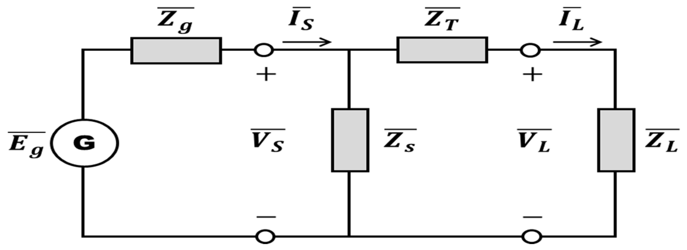
The virtual buses in the power sending and load parts are constructed with Equations (1)–(6) using the phasor measurement data. Figure 4 shows the TE circuit model of the electric power system.
As shown in Figure 4, and are the shunt and series impedances of the transmission line in the TE form, respectively. It is necessary to calculate the impedance of the generators and transformers and the in the generation part. Further, it is extremely important to calculate and because they could affect the TE impedance. Previously, for calculating those values, offline steady-state data were used. The generation part was decided; subsequently, and were obtained from the and injections. Subsequently, the average voltage of the generator is obtained. These values are inaccurate and difficult to apply for a real-time situation. Hence, a new concept to calculate and is proposed herein. In most power systems, the severe contingencies that cause the voltage instability arising from a reactive power imbalance occur in the load part instead of in the generation part. Therefore, it is possible to assume that and are not varying quickly when the power system suffers events such as sudden changes in voltage magnitude and load demand. Thus, they can be regarded as the same at times t and t′, as follows:
Using Kirchhoff’s voltage law (KVL), the equations for and can be expressed as follows:
By eliminating from Equations (9) and (10), the simultaneous equations can be solved and Equation (11) is obtained.
where and are the load voltage and current phasor measured at time t, respectively, while and are those measured at time t’, respectively. The equivalent voltage source can be derived as
The equations above assume that the TE does not vary between times t and t′; they are implemented over time to track the impedances. From Equation (11), if no changes occur in and , cannot be calculated. Events that change the voltage and current by more than some threshold should occur. In addition, oscillation is terminated because logic is required to determine the time t′ when transient stability does not affect the voltage and current. This concept is represented in Figure 5.
As shown in Figure 5, if the bus voltage is varying significantly or oscillating for a long time, it is difficult to determine the t′. The primary objective is to determine the normal condition time t and obtaining the appropriate time t′. When the data are measured, the occurrence of an event is verified. If no event occurs, then the present is the time t. If an event is occurring, wait until the oscillations of the phasors are less than the threshold ε such that the time t′. Figure 6 represents the framework for deciding the t′.
After the phasor data are obtained at times t and t′, the TE impedance is calculated. All data were measured and calculated to organize the TE circuit in Figure 4. Therefore, the TE circuit can be converted that shown in Figure 7.
Figure 4 shows that the equations are composed by the KCL (Kirchhoff’s current law) and KVL. The equations related with the TE circuit of the power systems are as follows:
The TE impedance can be obtained using Equations (1)–(17) above without any assumptions. These equations are simple to be applied in real time.
2.3. Voltage Stability Margin Calculation
The VSM can be computed using the TE circuit. The nose curve is drawn in theory using the TE voltages and impedances. To compare the operation and the nose point, the VSM should be obtained. The power systems are reduced to the TE form as shown in Figure 7. To simplify the equations for the nose curve, it is assumed that and , and the resistance of the transmission line is ignored. Subsequently, the following equations are obtained.
The complex power is absorbed by the load and decomposes into the following:
Eliminating from Equations (20) and (21) yields
This equation is a second-order equation with respect to . Changing this equation to a function composed of and PX using the quadratic equation yields
where . Using Equation (23), Figure 8 is constructed in the (P, V) space. The curves shown in Figure 8 are typically known as PV curves or nose curves.
As shown in Figure 8, the upper part of the curves corresponds to the solution with the plus sign in Equation (22) or the higher voltage solution. Meanwhile, the lower part corresponds to the solution with the minus sign, which is the low-voltage solution. These curves can be applied to the Thévenin impedances as every coefficient is calculated from the phasor measurement data. The curve can be drawn in real time using the TE circuit. Subsequently, the VSM can be computed by comparing the operation point and nose point, as shown in Figure 9.
As shown in Figure 9, the VSM value is correct when the loads are only of the constant power type. However, the power system loads are nonlinear. To obtain a more exact VSM, the load modeling parameters should be applied in this curve.
2.4. Load Modeling for Voltage Stability Margin
This subsection describes the measurement-based load modeling used in this study. In this model, a least-squares optimization method is applied to minimize the error between the measured and predicted values in the parameter estimation method. Because the phasor data of the load buses are obtained to establish the TE circuit, the data might be used to estimate the load modeling. It is assumed that the load model parameters estimated from the phasor data of the load buses are applicable to the VSM. Generally, the system frequency does not change significantly; thus, load fluctuations owing to small frequency variations cannot be captured accurately. Therefore, only the relationship between the load and voltage is considered in this study. The basic algorithm of the measurement-based approach is shown in Figure 10.
In Figure 10, the measurement-based load modeling structure is determined from the static load model. For a static load model, the exponential load model and ZIP load model are used widely. In this study, the ZIP model was selected for load modeling owing to the simplicity of its estimation. The ZIP model represents the load power as a polynomial equation of the voltages. The model structure is described below.
where . and are the active power and voltage in the steady state, respectively. In the parameter estimation procedure, three parameters (,, and ) of the load model are calculated using the measured data as input. The objective of the parameter estimation is to match the responses of the developed model with the measured responses. The objective function for minimizing the error is as follows:
where is the error function of parameter ; is the actual data at ; is the calculated data at with parameter p; is the total number of samples; is the parameter space. The least-squares method is applied to optimize the matching of the measured and simulated response values. The parameter space is defined as a permissible range of all the parameters to be estimated. The minimum parameter values in Equation (25) are considered as the desired solutions.
The Nose Curve Applying the Load Modeling
The VSM in Figure 9 assumes that the loads are composed of only constant power components. However, the loads of real power systems are not a constant power but the combination of various loads. The representative model reflecting this situation is the ZIP load model. In Figure 11, each red line represents the load characteristic curve for P_0. Two operating points are characterized by the same power but different load demands z. The load characteristic curve changes by increasing the load demand z, the system exhibits voltage instability during critical loading z_c, and the load characteristic curve becomes tangent to the PV curve. Subsequently, the voltage stability limit extends above the maximum deliverable power point.
In Figure 11, to calculate the voltage stability limit, Equation (24) is transformed to
where . To obtain the critical load demand , Equations (23) and (26) should be solved simultaneously. However, the equations are extremely complex to solve. Therefore, Equation (27) can be transformed to yield
It is assumed that ,, and are known values from the load modeling. The load modeling and and are obtained from Equation (23); thereby, we can compute the set . The maximum value of this set is the critical load demand .
The load characteristic curves, indicated by the red line in Figure 11, are obtained from Equation (29) and set .
3. Results and Discussion
The results of the voltage stability analysis of the practical system are investigated in this section. The Korean power system applies the algorithm proposed herein to verify its operation in real time. The Korean power system, which contains multiple buses, is reduced to a single bus equivalent system; hence, the TE circuit can be composed of TE impedances. Using that circuit, the VSM index is computed, and the margin is calculated and applied with the load modeling. The case study demonstrates that the circuit can predict a voltage collapse in the Korean power grid.
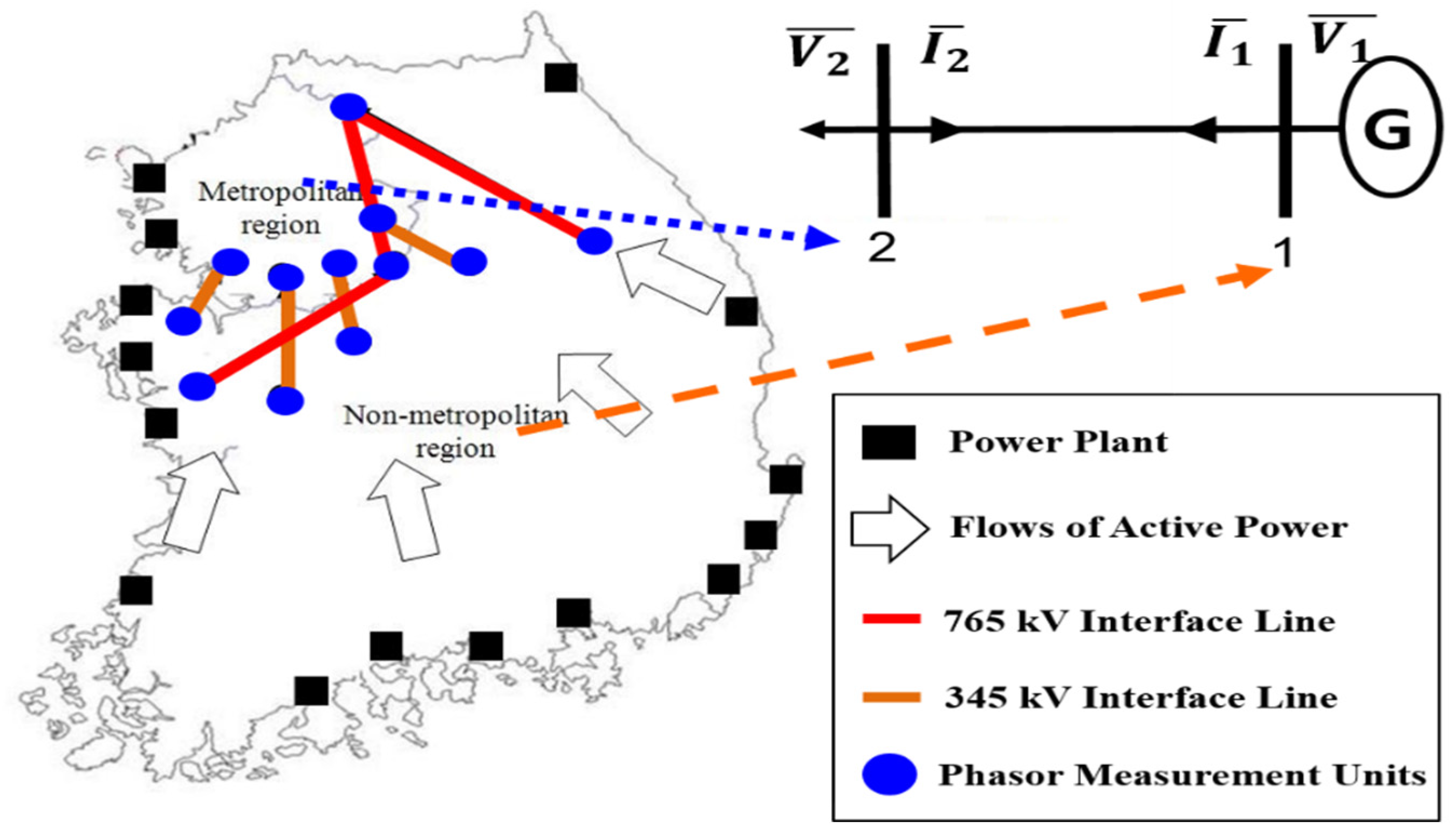
The characteristic of the Korean power system is that most of the load is concentrated in the metropolitan area in the northern part. Approximately 42% of the total loads are massed in this area. Only 20% of the total generations exist in this high-cost area. Further, most generations are gathered in the nonmetropolitan area located in the southern part. Therefore, the power flows from the south to north. Hence, a large amount of active power is transmitted through the interface lines connecting the metropolitan region and its neighboring region. The loading must be constrained by the thermal, voltage, and stability limits to operate the system securely because heavy power flowing into the region in the normal state can cause system insecurity if severe contingencies occur. In the Korean power system, the interface flow limit operation is considered under a fixed load demand condition [48]. Under these geographical circumstances, six major lines are constructed in the metropolitan area to supply large quantities of power. The six interface lines constitute the most important lines in the Korean power system. Figure 12 shows the diagram of the Korean power grid.
Figure 12 shows the characteristics of the Korean power system that consists of a major transmission line supplying most of the active power required for the metropolitan area. Power system operators in Korea are concerned that the heavy active power flow into the metropolitan area may intensify, and that the constraint of the interface flow will be a significant factor that results in congestion. Therefore, investigating both sides of those six lines is the best solution for monitoring the voltage stability in the Korean power system. For the case study, it is assumed that PMUs are installed on every receiving-end bus and sending-end bus of six major transmission lines. The voltages and currents are measured in the phasor waveform from every PMU, and the active power and reactive power are calculated.
3.1. Case 1
Case 1 is a scenario where the power system is rendered nearly unstable using the line trip and increasing the reactive power. A time-domain simulation is performed to assess the voltage stability. Figure 13 shows the variation in the voltage magnitude in the power sending part.
As shown in Figure 13, the two 4400-6950 circuits that are highly important interface lines were tripped after 5 s. Typically, the voltage stability problem of the Korean power system occurs on the 4400-6950 transmission line. Consequently, a PMU is installed on this line in case of an emergency. Subsequently, the reactive power loads increase to ~355 MVAR in the metropolitan area in 20 s. After 30 s, the voltage of the metropolitan area decreased rapidly to below 0.7 p.u. To investigate the voltage instability, an index based on the maximal power deliverable theory is used. This index shows whether a power system is stable. From this circuit theory, maximal power transfer occurs when |ZL| equals |ZTh|. The apparent impedance |ZL| is the proportion between the voltage and current phasors measured at the load bus. When the loading is normal, |ZL| is significantly greater than |ZTh|. In other words, the index is approximately zero. When the system suffers from voltage instability, the difference between the two impedances approaches zero, and the index is increased by ~1.0. Figure 14 shows this concept applied to case 1.
As shown in Figure 14, ZTh increases and ZL decreases, indicating that the system will become unstable. Subsequently, they are near each other at approximately t = 40 s, suggesting that the Z index approaches 1.0 and the system is nearly unstable. This voltage instability index is a real number, i.e., 0.0–1.0; if the index indicates a number over 1.0, the system will be unstable, theoretically. Similarly, an index under 1.0 indicates that the system is stable.
3.2. Case 2
Case B is a scenario where the power system is rendered unstable by applying a continuous line tripping. The voltage instability index from applying this scenario was observed and analyzed. The contingencies occur every 10 s. Table 1 shows the succession contingency scenario on the transmission lines.
As shown in Table 1, the contingency lists to be applied in the case-2 simulation are double circuit outages of 345-kV and 765-kV transmission lines. After the contingency occurs, the power system develops into a serious situation. Figure 15 shows that the bus voltage variation depends on the virtual bus in the power sending part.
As shown in Figure 15, the voltage magnitude decreases stepwise. This simulation terminated as voltage collapse occurred at approximately t = 88 s. Figure 16 shows the ZTh, ZL, and the Z index to monitor the power system situation.
As shown in Figure 16, the power system becomes unstable gradually because the ZTh increases while the ZL decreases. Their values match at approximately t = 82 s; it can be observed that the index increases as the transmission lines are tripping and finally indicates 1.0. Consequently, this implies that the index can be sufficient for monitoring the voltage instability as it demonstrates all contingencies. The results of the voltage instability index were similar to those of case 1.
3.3. Voltage Stability Margin
As mentioned earlier, the VSM should be obtained to compare the operation point and nose point. Using the results above, the PV curves are represented in Figure 17.
As shown in Figure 17, the nose curves are located at 0, 10, 20, 30, 40, 50, and 60 s from the right side. The circle indicates the operating point. The scale of the x axis is per unit; therefore, the present operating point is approximately 6165 MW. As shown in the figure, the VSM is large at first time. However, the margin decreases with time, and almost vanishes at 60 s. Table 2 shows the specific margin at each curve.
As shown in Table 2, the margin decreased steadily until the simulation ended and had even exhibited a minus value. Theoretically, the margin cannot be smaller than zero, as this implies that the system does not have an operation point and voltage instability occurs. However, this simulation was operated dynamically, and the load is not a constant power. The load parameters should be applied in the PV curves. Figure 18 shows both the PV and load characteristic curves.
As shown in Figure 18, the first red curve is the operating curve and the other red lines are the maximum load demand curves. Even though the PV curve is reduced to the last one (left end blue curve), an operating point exists. Table 3 shows the margins with each load character curve.
From Table 2, the maximum load demand factors with each load character curve are arranged. The proportions of the ZIP model parameter are 35.1%, 14.1%, and 50.8% for the constant impedance, current, and power, respectively. The VSM is expressed in the load demand factor because it is not merely an active power such as a constant power; thus, it cannot be matched with the MW units.
3.4. Discussion
The abovementioned analysis results are summarized in Table 4. As shown from these results, the index may be used to monitor the voltage stability, thus reflecting the power system situation in real time with fast computations.
As shown in Table 4, voltage instability occurs when the index is 1.0. In theory, voltage instability occurs when the index is 1.0. However, voltage instability might occur even though the index is below 1.0 in a practical situation. Therefore, the system operator requires more absolute values. Hence, the most severe VSI should be added to provide a threshold value to the system operators. Figure 19 shows the results of the measured and threshold values under a severe contingency in the Korean power system.
In Figure 19, the red line is the index from the measured data and the blue line is the threshold value. As shown, the system is stable in terms of voltage stability. Consequently, it may be useful to monitor the indicators for deciding the appropriate countermeasures based on the phasor measurement data. Additionally, because the system operator can actively cope with emergencies using the proposed method, it can prevent enormous economic losses by performing the appropriate countermeasures to prevent a wide-area outage caused by voltage instability. Thus, utilizing the proposed method within the Korean power system might protect the system efficiently.
Currently, the Korean electric power system has completed the development of the wide-area monitoring system (WAMS) technology based on PMUs to assess voltage stability. Following the WAMS, the wide-area monitoring and control (WAMAC) technology is being developed. Further, the wide-area monitoring protection and control (WAMPAC) technology is being planned as the final goal of the R&D roadmap. Table 5 shows the stability and control measures for each technology phase.
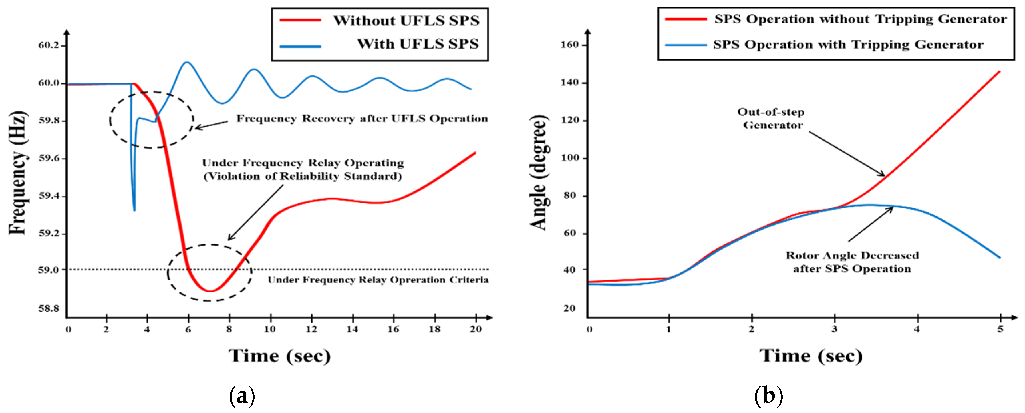
As mentioned above, when major high-voltage transmission lines are tripped after a fault, it might result in a large-scale blackout that may cause catastrophic damage to the entire system. Thus, appropriate countermeasures are required to ensure the frequency and angle stability of a large-scale power system [49,50]. Hence, a special protection scheme is applied based on the proposed method to secure stability. Depending on each step, load shedding and generator tripping SPS may be used. The comparison results of with and without the SPS for ensuring stability are shown in Figure 20.
As shown in Figure 19, the system is stable when SPS is applied. When the system experiences low-frequency problems a few seconds after critical events, the UFLS scheme is activated. In the Korean power system, applying the WAMAC technology based on the PMU might effectively ensure its frequency stability. The proposed method of stability index can be used to monitor the frequency state of the system. In addition, PMU applications enable the implementation of the load shedding strategy for emergency situations where load shedding based on the stability margin must be decided. Thus, it is possible to identify a suitable location for the control scheme used as a criterion for UFLS.
Further, the generator tripping SPS might be used as a protection strategy in the WAMPAC system by ensuring the angle stability. This final stage is reflected on the grid state for assessing the stability and determined the adequate SPS. When a contingency occurs, the generator electrical output and angle increase. Subsequently, increasing the angular swings in some generators may result in the loss of their synchronism. As shown from the results, the equilibrium state between the electromagnetic torque and mechanical torque of each synchronous machine in the system is restored by the SPS. This implies that the acceleration energy accumulated during the fault must be released quickly by tripping more generators. Thus, the proposed method may be applied for the stabilization to control the detected instability state by calculating the stability margin. The proposed method allows for the stabilizing of the system to be elaborated; further, it can be extended for conceptual virtual loads. In summary, the advanced SPS connected with the WAMPAC system for real-time assessment and protection control can ensure angle stability.
4. Conclusions
A method estimating the TE impedance from a multiple bus system such as the Korean power system and for calculating the VSM in real time was proposed herein. The VSM could be computed using the TE circuit. A nose curve was constructed based on TE circuit using the TE voltages and impedances. In addition, to calculate the TE impedance and circuit modeling was applied. The index indicating system stability using the TE impedance was introduced. These indicators were used throughout the proposed process and calculated by the PMU data through the measured voltage and current waveforms. Thus, the calculated voltage instability index could be used as a useful index by system operators in critical decision making. Additionally, the performances of the proposed method were tested using time-domain simulations of the Korean power system, and the results demonstrated the effectiveness of the TE impedance estimation method.
Future research work will focus on the applied smart grid technology. The smart grid, where information communication technology is being integrated on the conventional grid, enables the exchange of real-time power information between a power supplier and consumer bi-directionally. Hence, to control the power system that changes hourly, a monitoring system is highly important. As such, the monitoring system should be more powerful, fast, accurate, and robust. The development of this study can contribute to the establishment of an optimal control strategy to prevent wide-area power outages and create more efficient power systems.
Author Contributions
Y.L. conceived and designed the research, conducted simulations, and wrote the paper. S.H. contributed analysis tools and analyzed the data, improved the theoretical part, and supervised the research.
Funding
This work was supported by the National Research Foundation of Korea [2017R1D1A1B03034460] and Korea Electric Power Corporation [Grant number: R18XA06-65].
Conflicts of Interest
The authors declare no conflict of interest.
References
- Van Cutsem, T. Voltage instability: Phenomena, countermeasures, and analysis methods. Proc. IEEE 2000, 88, 208–227. [Google Scholar] [CrossRef]
- Taylor, C.; Erickson, D.; Martin, K.E.; Wilson, R. WACS-wide-area stability and voltage control system: R&D and online demonstration. Proc. IEEE 2005, 93, 892–906. [Google Scholar]
- Sinha, A.K.; Hazarika, D. A comparative study of voltage stability indices in a power system. Int. J. Electr. Power Energy Syst. 2000, 22, 589–596. [Google Scholar] [CrossRef]
- Zarate, L.; Castro, C. A critical evaluation of a maximum loading point estimation method for voltage stability analysis. Electr. Power Syst. Res. 2004, 70, 195–202. [Google Scholar] [CrossRef]
- De Souza, Z.; De Souza, S.; Da Silva, A. On-line voltage stability monitoring. IEEE Trans. Power Syst. 2000, 15, 1300–1305. [Google Scholar] [CrossRef]
- Haque, H. On-line monitoring of maximum permissible loading of a power system within voltage stability limits. IEEE Proc. Gener. Transm. Distrib. 2003, 150, 107–112. [Google Scholar] [CrossRef]
- Gao, B.; Morison, K.; Kunder, P. Voltage stability evaluation using modal analysis. IEEE Trans. Power Syst. 1992, 7, 1529–1542. [Google Scholar] [CrossRef]
- Chebbo, M.; Irving, R.; Sterling, H. Voltage collapse proximity indicator: Behaviour and implications. IEEE Proc. C 1992, 139, 241–252. [Google Scholar] [CrossRef]
- Vu, K.; Begovic, M.; Novosel, D.; Saha, M. Use of local measurements to estimate voltage-stability margin. IEEE Trans. Power Syst. 1999, 14, 1029–1035. [Google Scholar] [CrossRef]
- Corsi, S.; Taranto, N. A real-time voltage instability identification algorithm based on local phasor measurements. IEEE Trans. Power Syst. 2008, 23, 1271–1279. [Google Scholar] [CrossRef]
- Wiszniewski, A. New criteria of voltage stability margin for the purpose of load shedding. IEEE Trans. Power Deliv. 2007, 22, 1367–1371. [Google Scholar] [CrossRef]
- Moghavvemi, M.; Faruque, O. Real-time contingency evaluation and ranking technique. IEEE Proc. Gener. Transm. Distrib. 1998, 145, 517–524. [Google Scholar] [CrossRef]
- Smon, I.; Verbic, G.; Gubina, F. Local voltage-stability index using Tellegen’s theorem. IEEE Trans. Power Syst. 2006, 21, 1267–1275. [Google Scholar] [CrossRef]
- Wang, Y.; Li, W.; Lu, J. A new node voltage stability index based on local voltage phasors. Electr. Power Syst. Res. 2009, 79, 265–271. [Google Scholar] [CrossRef]
- Fu, L.; Pal, C.; Cory, J. Phasor measurement application for power system voltage stability monitoring. In Proceedings of the Power and Energy Society General Meeting-Conversion and Delivery of Electrical Energy in the 21st Century, Pittsburgh, PA, USA, 20–24 July 2008; pp. 1–8. [Google Scholar]
- Verbic, G.; Gubina, F. A new concept of voltage-collapse protection based on local phasors. IEEE Trans. Power Syst. 2004, 19, 576–581. [Google Scholar] [CrossRef]
- Julian, E.; Schulz, P.; Vu, T.; Quaintance, H.; Bhatt, B.; Novosel, D. Quantifying proximity to voltage collapse using the voltage instability predictor (VIP). In Proceedings of the 2000 Power Engineering Society Summer Meeting, Seattle, WA, USA, 16–20 July 2000; pp. 931–936. [Google Scholar]
- Vu, K.; Novosel, D. Voltage Instability Predictor (vip)-Method and System for Performing Adaptive Control to Improve Voltage Stability in Power Systems. U.S. Patent No. 6,219,591, 17 April 2001. [Google Scholar]
- Larsson, M.; Rehtanz, C.; Bertsch, J. Monitoring and operation of transmission corridors. In Proceedings of the IEEE Bologna Power Tech Conference, Bologna, Italy, 23–26 June 2003; Volume 3. [Google Scholar]
- Larsson, M.; Rehtanz, C.; Bertsch, J. Real-time voltage stability assessment of transmission corridors. IFAC Proc. Vol. 2003, 36, 27–32. [Google Scholar] [CrossRef]
- Wang, Y.; Pordanjani, R.; Li, W.; Xu, W.; Chen, T.; Vaahedi, E.; Gurney, J. Voltage stability monitoring based on the concept of coupled single-port circuit. IEEE Trans. Power Syst. 2011, 26, 2154–2163. [Google Scholar] [CrossRef]
- Yang, J.; Li, W.; Chen, T.; Xu, W.; Wu, M. Online estimation and application of power grid impedance matrices based on synchronised phasor measurements. IET Gen. Transm. Distrib. 2010, 4, 1052–1059. [Google Scholar] [CrossRef]
- Mou, X.; Li, W.; Li, Z. A preliminary study on the Thevenin equivalent impedance for power systems monitoring. In Proceedings of the 2011 4th International Conference on Electric Utility Deregulation and Restructuring and Power Technologies, Weihai, Shandong, China, 6–9 July 2011; pp. 730–733. [Google Scholar]
- Huang, L.; Xu, J.; Sun, Y.; Cui, T.; Dai, F. Online monitoring of wide-area voltage stability based on short circuit capacity. In Proceedings of the 2011 Asia-Pacific Power and Energy Engineering Conference, Wuhan, China, 25–28 March 2011; pp. 1–5. [Google Scholar]
- Zhou, Q.; Annakkage, D.; Rajapakse, D. Online monitoring of voltage stability margin using an artificial neural network. IEEE Trans. Power Syst. 2010, 25, 1566–1574. [Google Scholar] [CrossRef]
- Seethalekshmi, K.; Singh, N.; Srivastava, C. A synchrophasor assisted frequency and voltage stability based load shedding scheme for self-healing of power system. IEEE Trans. Smart Grid. 2011, 2, 221–230. [Google Scholar] [CrossRef]
- Baldwin, L.; Mili, L.; Boisen, B.; Adapa, R. Power system observability with minimal phasor measurement placement. IEEE Trans. Power Syst. 1993, 8, 707–715. [Google Scholar] [CrossRef]
- Khatib, R.; Nuqui, F.; Ingram, R.; Phadke, G. Real-time estimation of security from voltage collapse using synchronized phasor measurements. In Proceedings of the Power Engineering Society General Meeting, Denver, CO, USA, 6–10 June 2004; pp. 582–588. [Google Scholar]
- Glavic, M.; Van Cutsem, T. Wide-area detection of voltage instability from synchronized phasor measurements. Part I: Principle. IEEE Trans. Power Syst. 2009, 24, 1408–1416. [Google Scholar] [CrossRef]
- Glavic, M.; Van Cutsem, T. Wide-area detection of voltage instability from synchronized phasor measurements. Part II: Simulation results. IEEE Trans. Power Syst. 2009, 24, 1417–1425. [Google Scholar] [CrossRef]
- Eissa, M.; Masoud, E.; Elanwar, M. A novel back up wide area protection technique for power transmission grids using phasor measurement unit. IEEE Trans. Power Deliv. 2010, 25, 270–278. [Google Scholar] [CrossRef]
- Dengjun, Y.; Ping, J.; Feng, W. Real time power angle measurement of a synchronous generator based on GPS clock signal and tachometer. Autom. Electr. Power Syst. 2002, 26, 3840. [Google Scholar]
- Kamwa, I.; Beland, J.; McNabb, D. PMU-based vulnerability assessment using wide-area severity indices and tracking modal analysis. In Proceedings of the 2006 IEEE PES Power Systems Conference and Exposition, Atlanta, GA, USA, 29 October–1 November 2006; pp. 139–149. [Google Scholar]
- Su, H.Y.; Liu, T.Y. A PMU-Based Method for Smart Transmission Grid Voltage Security Visualization and Monitoring. Energies 2017, 10, 1103. [Google Scholar] [CrossRef]
- Perez, A.; Johannsson, H.; Qstergaard, J.; Glavic, M.; Van Cutsem, T. Improved Thévenin equivalent methods for real-time voltage stability assessment. In Proceedings of the 2016 IEEE International Energy Conference, Leuven, Belgium, 4–8 April 2016; pp. 1–6. [Google Scholar]
- Su, H.; Liu, C. Estimating the voltage stability margin using PMU measurements. IEEE Trans. Power Syst. 2016, 31, 3221–3229. [Google Scholar] [CrossRef]
- Burchett, M.; Douglas, D.; Ghiocel, G.; Liehr, W.J.; Chow, J.H.; Kosterev, D.; Matthews, G.H. An Optimal Thévenin Equivalent Estimation Method and its Application to the Voltage Stability Analysis of a Wind Hub. IEEE Trans. Power Syst. 2018, 33, 3644–3652. [Google Scholar] [CrossRef]
- Abdelkader, S.M.; Morrow, D.J. Online Thévenin equivalent determination considering system side changes and measurement errors. IEEE Trans. Power Syst. 2015, 30, 2716–2725. [Google Scholar] [CrossRef]
- Alinezhad, B.; Karegar, H.K. On-line Thevenin impedance estimation based on PMU data and phase drift correction. IEEE Trans. Smart Grid 2018, 9, 1033–1042. [Google Scholar] [CrossRef]
- Perez, A.; Johannsson, H.; Qstergaard, J.; Martin, K. Improved method for considering PMU’s uncertainty and its effect on real-time stability assessment methods based on Thévenin equivalent. In Proceedings of the 2015 IEEE Eindhoven PowerTech, Eindhoven, The Netherlands, 29 June–2 July 2015; pp. 1–5. [Google Scholar]
- Hu, F.; Sun, K.; Del, A.; Farantatos, E. Measurement-based real-time voltage stability monitoring for load areas. IEEE Trans. Power Syst. 2016, 31, 2787–2798. [Google Scholar] [CrossRef]
- Fan, Y.; Liu, S.; Qin, L.; Li, H.; Qiu, H. A novel online estimation scheme for static voltage stability margin based on relationships exploration in a large data set. IEEE Trans. Power Syst. 2015, 30, 1380–1393. [Google Scholar] [CrossRef]
- Bedekar, P.P.; Telang, A.S. Load flow based voltage stability indices to analyze voltage stability and voltage security of the power system. In Proceedings of the 2015 5th Nirma University International Conference on Engineering, Ahmedabad, India, 26–28 November 2015; pp. 1–6. [Google Scholar]
- Li, S.; Ajjarapu, V.; Djukanovic, M. Adaptive online monitoring of voltage stability margin via local regression. IEEE Trans. Power Syst. 2018, 33, 701–713. [Google Scholar] [CrossRef]
- Dong, X.; Wang, C.; Yun, Z.; Han, X.; Liang, J.; Wang, Y.; Zhao, P. Calculation of optimal load margin on improved continuation power flow model. Int. J. Electr. Power Energy Syst. 2018, 94, 225–233. [Google Scholar] [CrossRef]
- Kamel, M.; Karrar, A.A.; Eltom, A.H. Development and application of a new voltage stability index for on-line monitoring and shedding. IEEE Trans. Power Syst. 2018, 33, 1231–1241. [Google Scholar] [CrossRef]
- Han, S.; Lee, B.; Kim, S.; Moon, Y. Real time wide area voltage stability index in the Korean metropolitan area. J. Electr. Eng. Technol. 2009, 4, 451–456. [Google Scholar] [CrossRef]
- Lee, B.; Song, H.; Kwon, S.H.; Jang, G.; Kim, J.H.; Ajjarapu, V. A study on determination of interface flow limits in the KEPCO system using modified continuation power flow (MCPF). IEEE Trans. Power Syst. 2002, 17, 557–564. [Google Scholar]
- Choi, D.; Lee, S.; Kang, Y.; Park, W. Analysis on special protection scheme of korea electric power system by fully utilizing STATCOM in a generation side. IEEE Trans. Power Syst. 2017, 32, 1882–1890. [Google Scholar] [CrossRef]
- Mohammadi, F.; Zheng, C. Stability Analysis of Electric Power System. In Proceedings of the 2018 4th National Conference on Technology in Electrical and Computer Engineering, Bern, Switzerland, 20–22 December 2018; pp. 1–8. [Google Scholar]
Figure 1.
Conceptual diagram of power system divided into four groups.
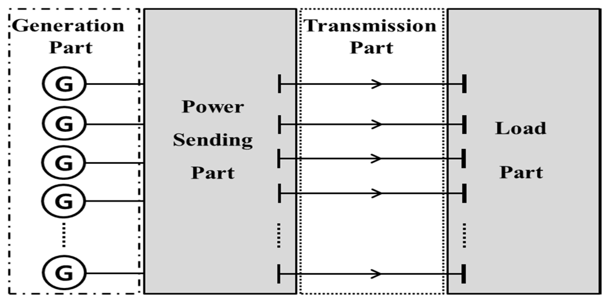
Figure 2.
Configuration of virtual single bus systems.
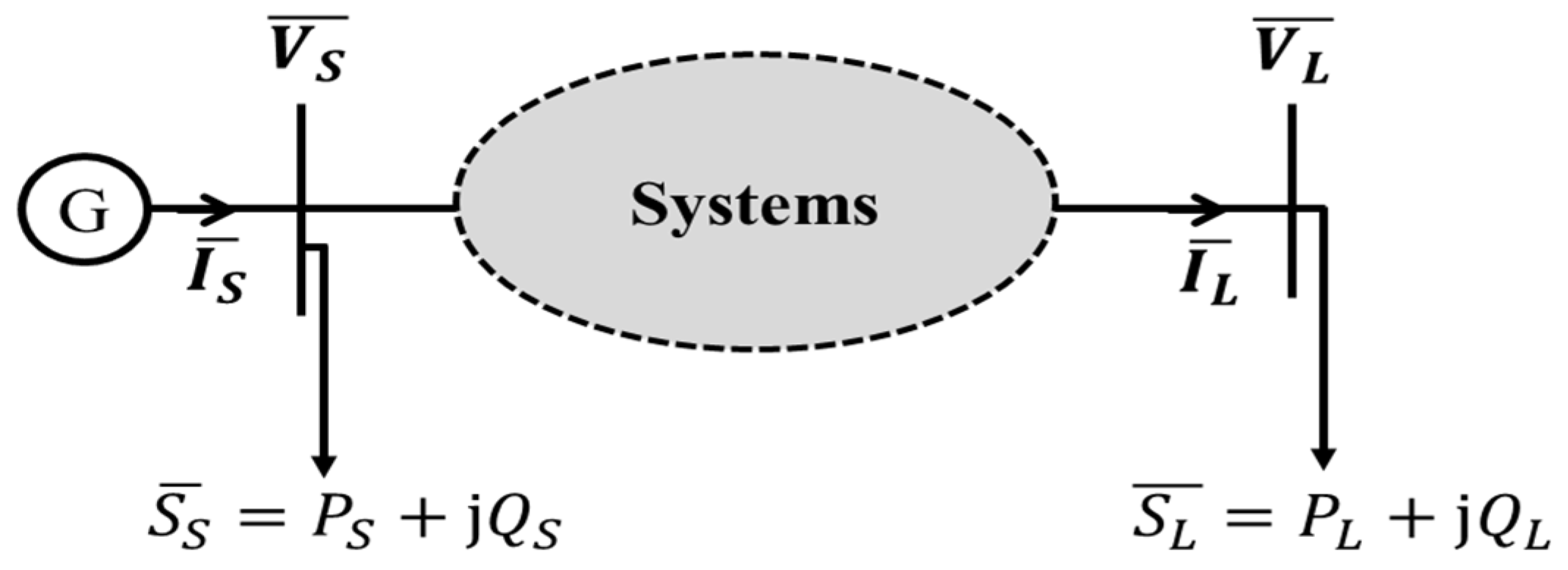
Figure 3.
Multiple bus systems with the measurement units.
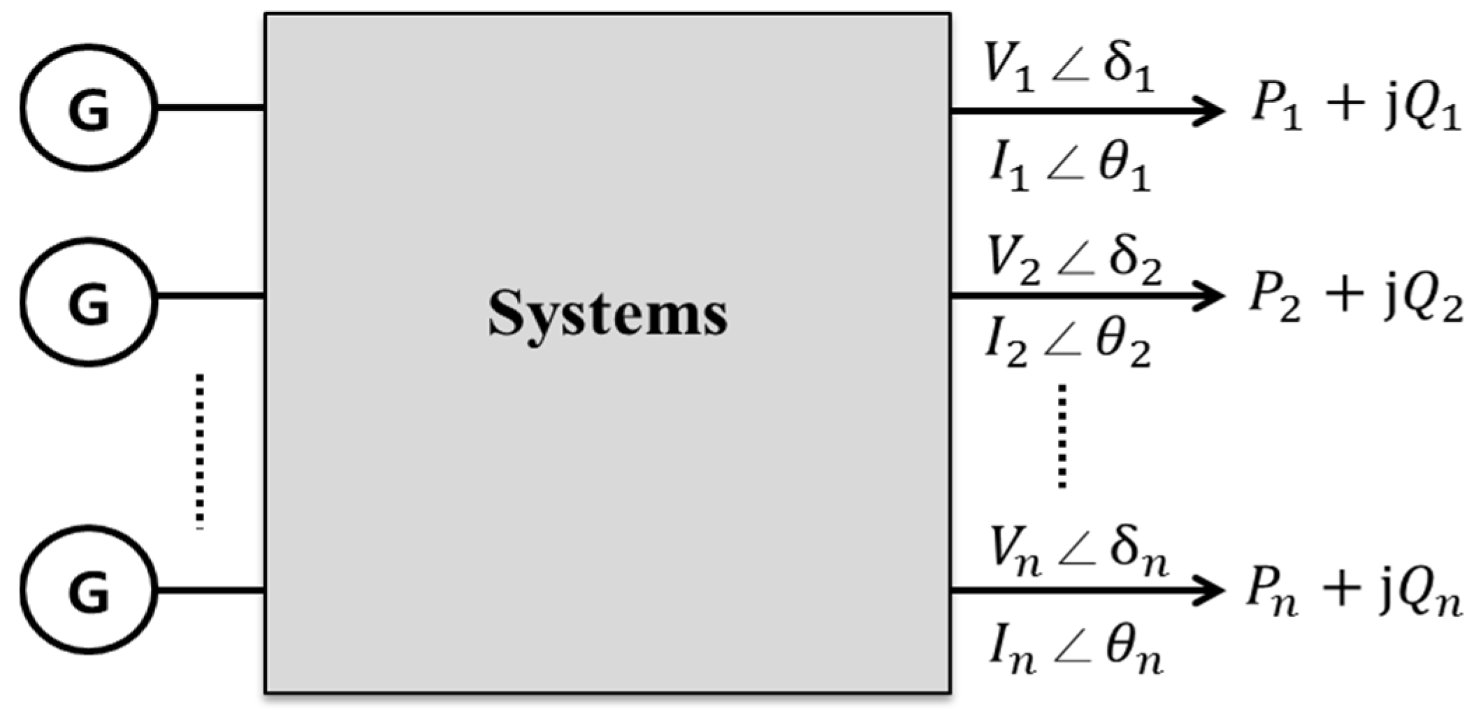
Figure 4.
Thévenin equivalent circuit model of power system.

Figure 5.
Concept of Vs’ and time t′.
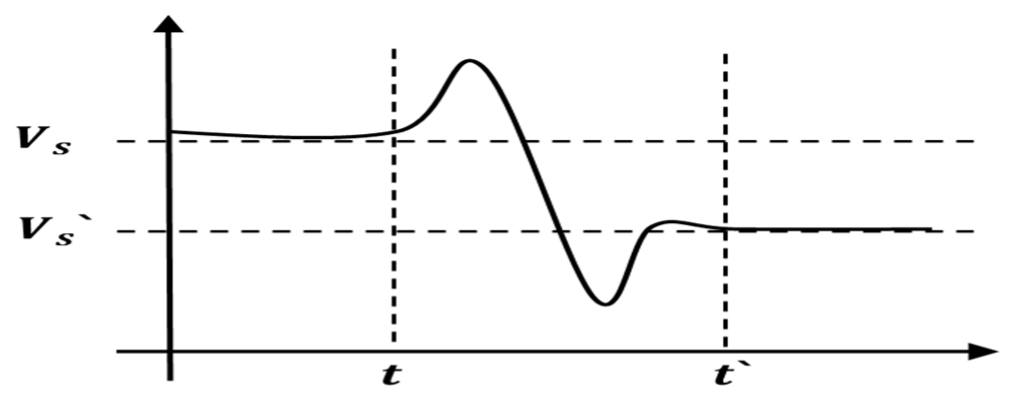
Figure 6.
Flow chart of deciding the phasors at time t and t′.

Figure 7.
Thévenin equivalent circuit of the power systems.

Figure 8.
Typical PV curve with the tan Φ.
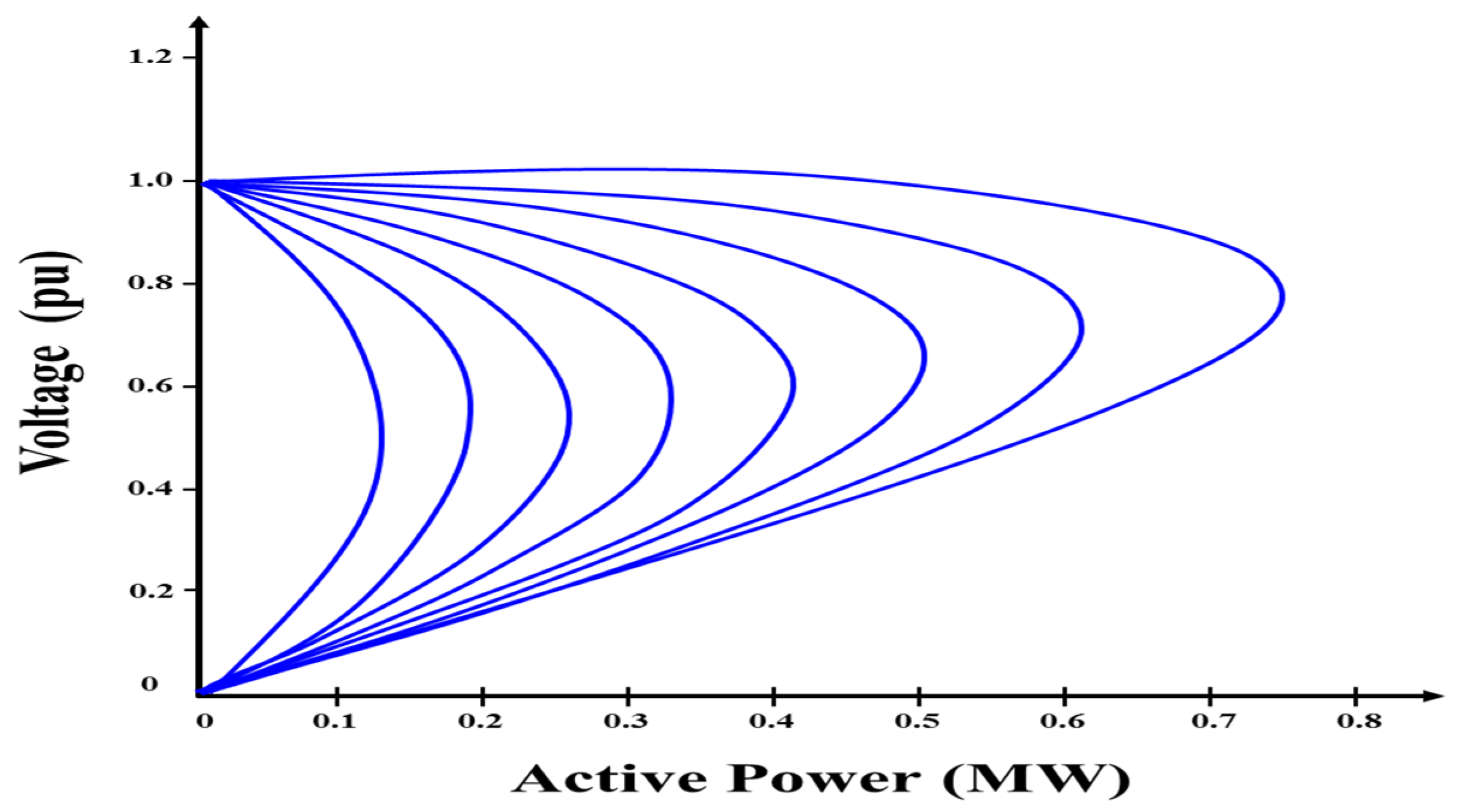
Figure 9.
Voltage stability margin with PV curve.
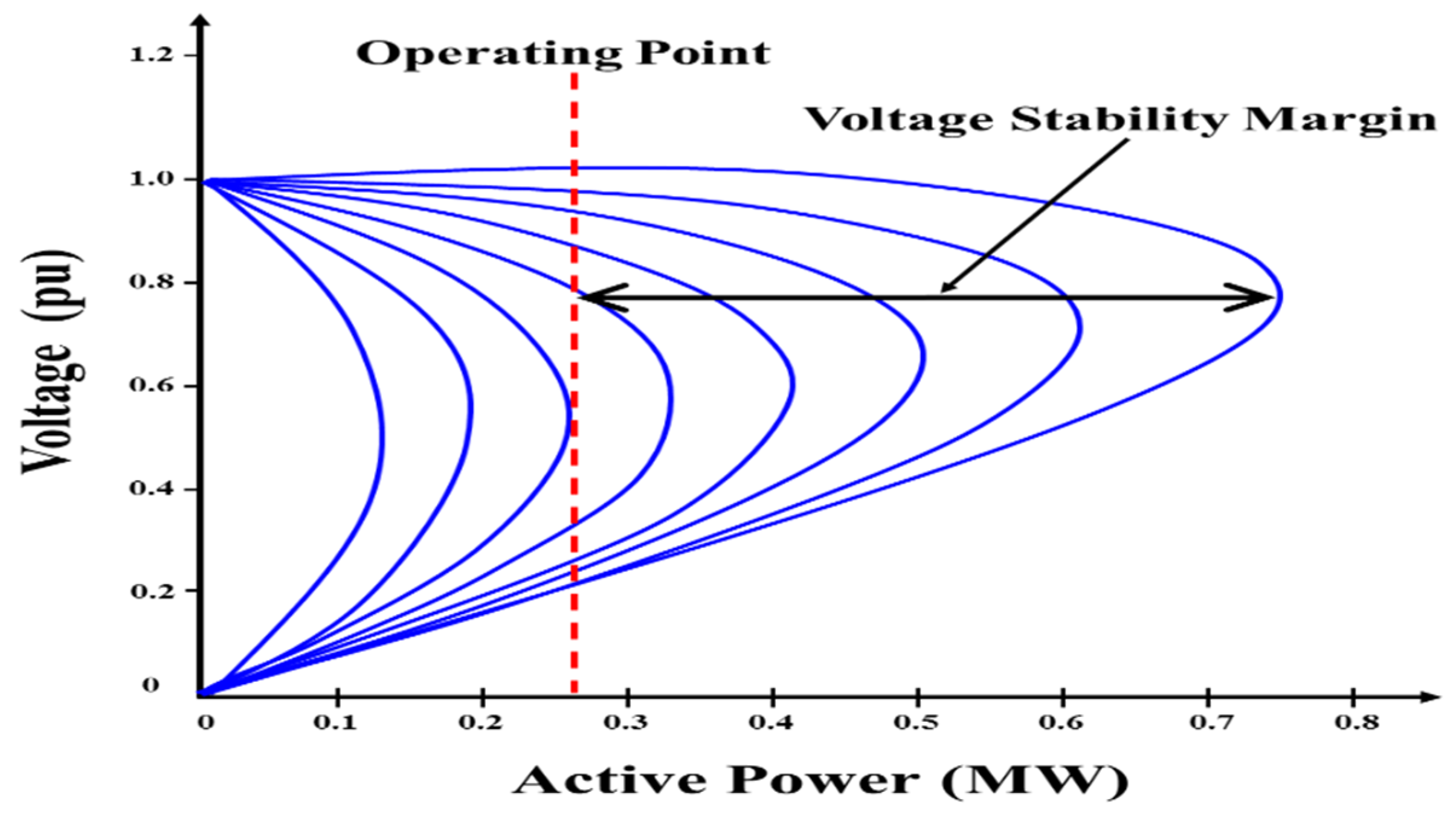
Figure 10.
Measurement-based approach load modeling algorithm.
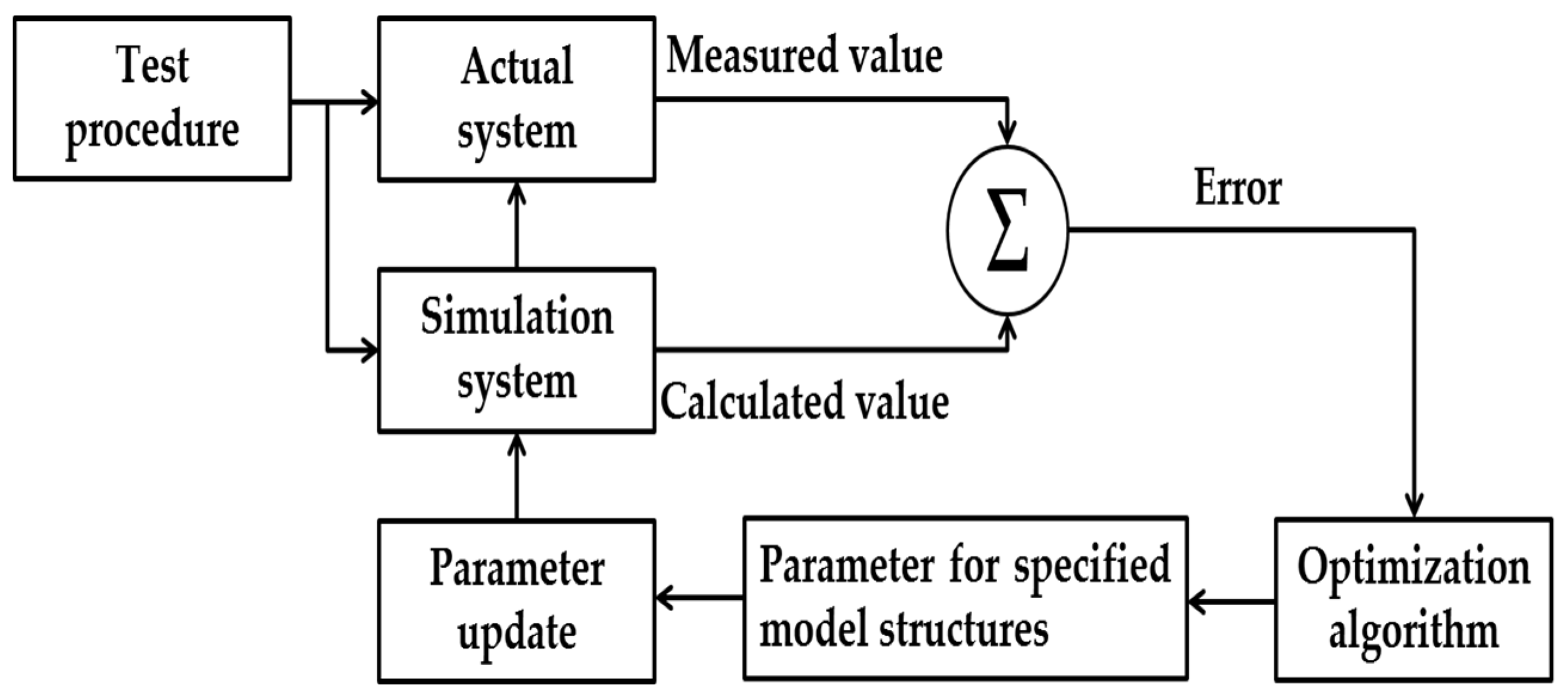
Figure 11.
PV curves with the ZIP load.
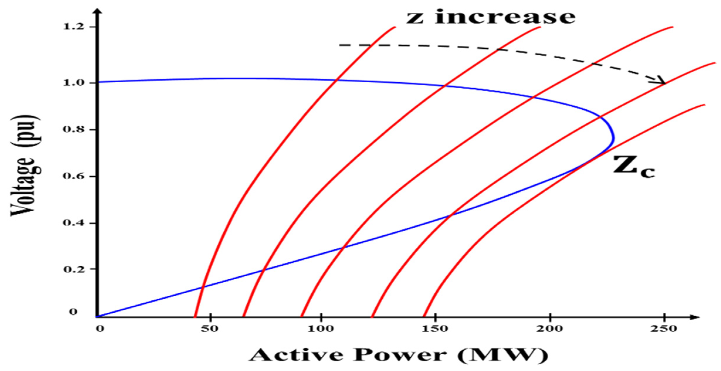
Figure 12.
Korean power system grid and the major transmission lines.

Figure 13.
Voltage magnitude variation of virtual bus.
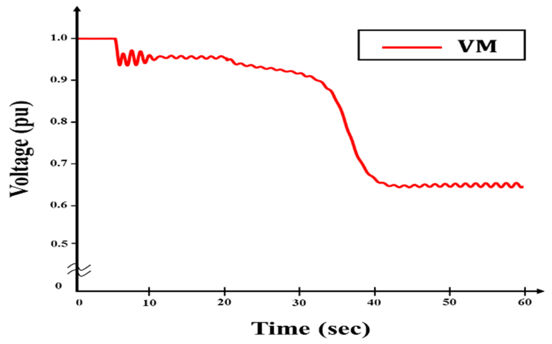
Figure 14.
Progress of the index in case 1. (a) ZTh and ZL. (b) Z index.
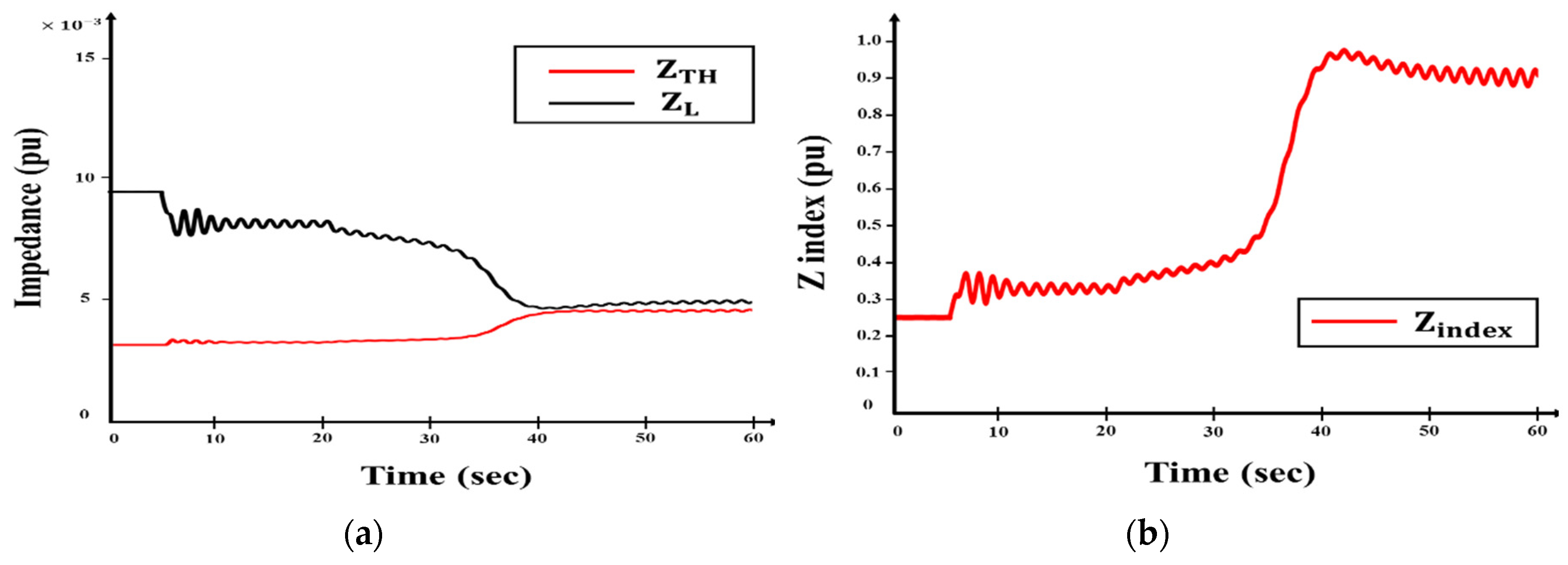
Figure 15.
Voltage magnitude of virtual bus in the power sending part depends on the contingencies.
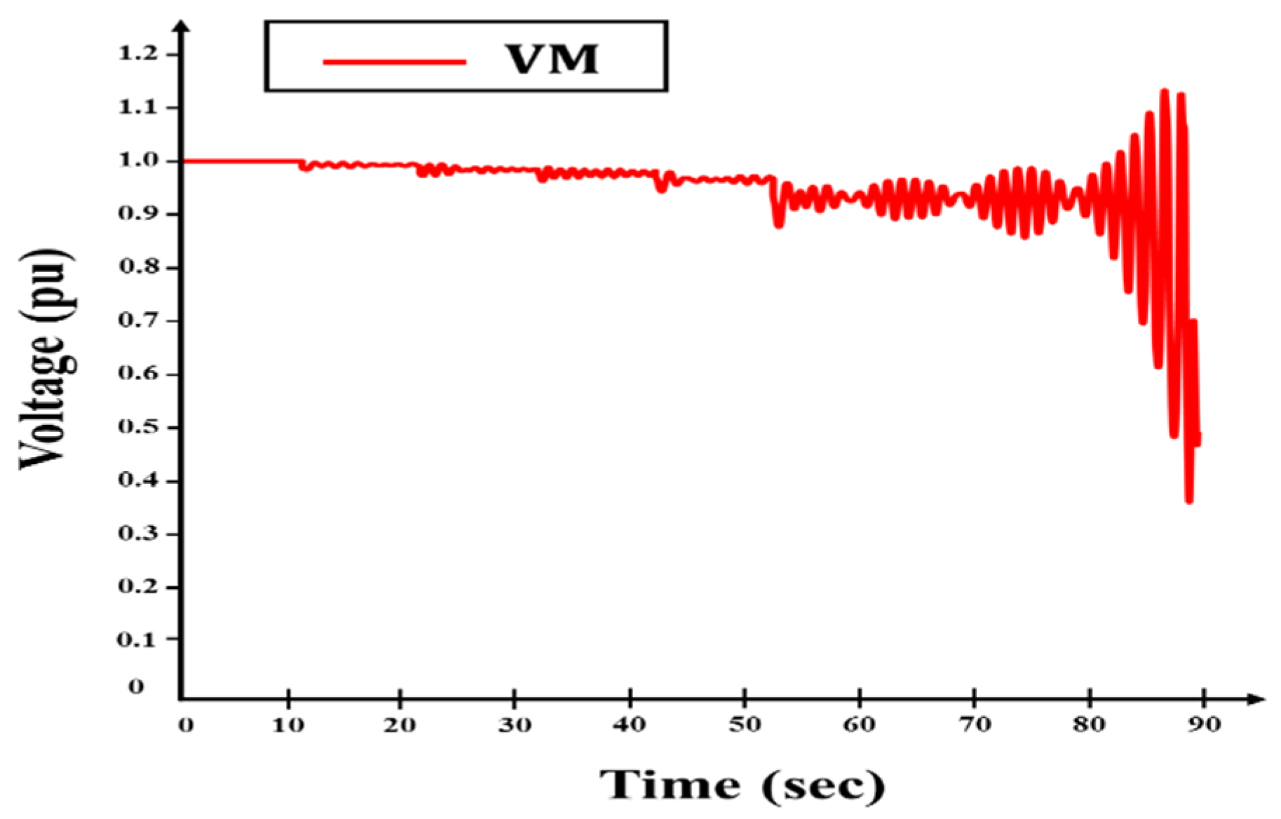
Figure 16.
Progress of the index in case 2. (a) ZTh and ZL. (b) Z index.
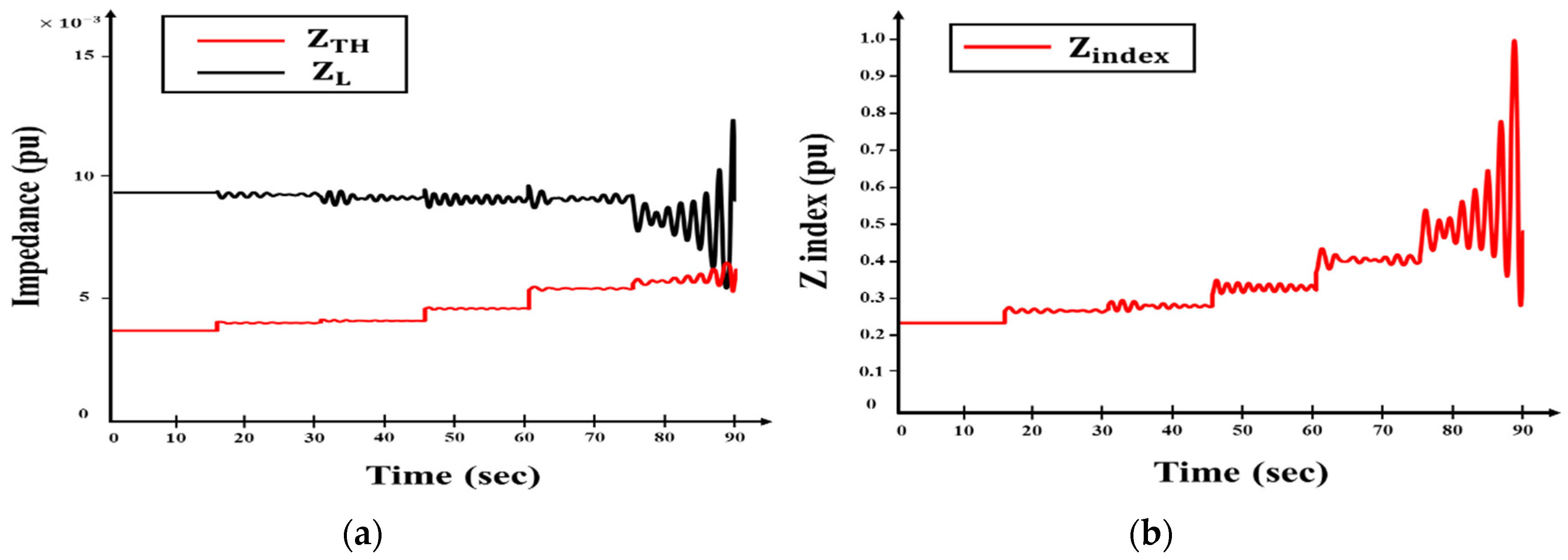
Figure 17.
PV curves using Thévenin equivalent impedance.

Figure 18.
PV curves and load characteristic curves.
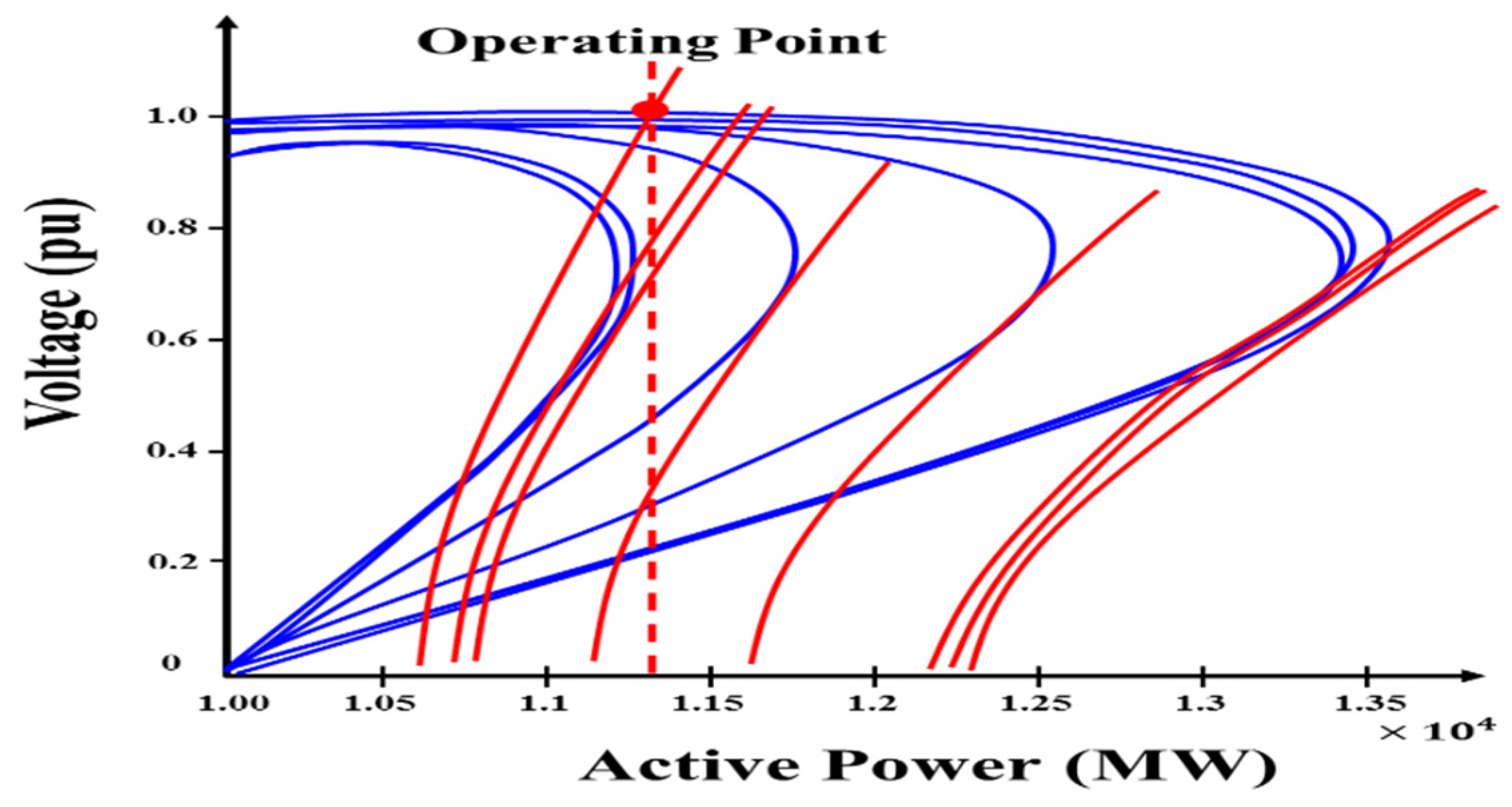
Figure 19.
Observation for the measured data and threshold value with severe contingency.

Figure 20.
Frequency and angle responses for the cases with and without special protection scheme based on proposed method; (a) frequency, (b) angle.
Figure 20.
Frequency and angle responses for the cases with and without special protection scheme based on proposed method; (a) frequency, (b) angle.

Table 1.
Series contingency scenario on the transmission lines.
| List | Time (s) | Contingency Line | Circuits |
|---|---|---|---|
| 1 | 10 | 1020-5010 | 2 |
| 2 | 20 | 4010-6030 | 2 |
| 3 | 30 | 4400-6950 | 2 |
| 4 | 40 | 4650-4950 | 2 |
| 5 | 50 | 4450-4650 | 2 |
Table 2.
Specific margins with each PV curve.
| Time (s) | Margins (MW) |
|---|---|
| 0 | 2177 |
| 10 | 2080 |
| 20 | 2045 |
| 30 | 1191 |
| 40 | 429 |
| 50 | −44 |
| 60 | −96 |
Table 3.
Margins with each load character curve.
| Time (s) | Margins (MW) |
|---|---|
| 0 | 3075 |
| 10 | 2999 |
| 20 | 2988 |
| 30 | 1873 |
| 40 | 888 |
| 50 | 291 |
| 60 | 246 |
Table 4.
Comparison of the Case 1 and Case 2.
| Classification | Voltage Stability Results (Index) | Voltage Stability Margin (MW) |
|---|---|---|
| Case 1 | Unstable (1.0) | 583 |
| Case 2 | Unstable (1.0) | 246 |
Table 5.
Each technology phase target for phasor measurement unit (PMU) application.
| Classification | 1st Phase | 2nd Phase | 3rd Phase |
|---|---|---|---|
| PMU Application | Wide Area MonitoringSystem | Wide Area Monitoring and Control | Wide Area Monitoring Protection and Control |
| Ensure Stability | Voltage Stability | Frequency Stability | Angle Stability |
| Countermeasure | Stability Assessment | Under Frequency Load Shedding (UFLS) | Tripping Generation Units |
© 2019 by the authors. Licensee MDPI, Basel, Switzerland. This article is an open access article distributed under the terms and conditions of the Creative Commons Attribution (CC BY) license (http://creativecommons.org/licenses/by/4.0/).
Share and Cite
MDPI and ACS Style
Lee, Y.; Han, S. Real-Time Voltage Stability Assessment Method for the Korean Power System Based on Estimation of Thévenin Equivalent Impedance. Appl. Sci. 2019, 9, 1671. https://doi.org/10.3390/app9081671
AMA Style
Lee Y, Han S. Real-Time Voltage Stability Assessment Method for the Korean Power System Based on Estimation of Thévenin Equivalent Impedance. Applied Sciences. 2019; 9(8):1671. https://doi.org/10.3390/app9081671
Chicago/Turabian StyleLee, Yunhwan, and Sangwook Han. 2019. "Real-Time Voltage Stability Assessment Method for the Korean Power System Based on Estimation of Thévenin Equivalent Impedance" Applied Sciences 9, no. 8: 1671. https://doi.org/10.3390/app9081671
Note that from the first issue of 2016, this journal uses article numbers instead of page numbers. See further details here.