Impact Location on a Fan-Ring Shaped High-Stiffened Panel Using Adaptive Energy Compensation Threshold Filtering Method


1
State Key Laboratory of Precision Measurement Technology and Instrument, Tianjin University, Tianjin 300072, China
2
Beijing Institute of Spacecraft Environment Engineering, Beijing 100094, China
3
Department of Materials Science and Engineering, The Ohio State University, 2041 N. College Road, Columbus, OH 43210, USA
*
Author to whom correspondence should be addressed.
Appl. Sci. 2019, 9(9), 1763; https://doi.org/10.3390/app9091763
Submission received: 30 March 2019
/
Revised: 25 April 2019
/
Accepted: 25 April 2019
/
Published: 28 April 2019
(This article belongs to the Special Issue Structural Damage Detection and Health Monitoring)
Abstract
:The increase in the number of space debris is a serious threat to the safe operation of in-orbit spacecraft. The propagation law of the impact signal in the stiffened panel of the spacecraft’s sealed bulkhead is very complicated, and there is less research on the impact source location in the high-stiffened panel. In this paper, an adaptive energy compensation threshold filtering (AECTF) method based on acoustic emission is proposed, which can realize large-scale, fast and accurate locating of the impact source on the stiffened panel with less resource consumption. The influence law of the stiffeners on the lamb wave is analyzed by finite element simulation, and the Lamb wave energy factor curve is obtained. The correctness of the simulation is verified by the locating experiment on the impact point. The results show that the proposed AECTF method has better adaptability and can correctly locate the impact points in complicated locations. By selecting the appropriate frequency band to filter the signal, the locating accuracy and stability can be improved. When the frequency band is 100–200 kHz, the locating result is optimal, the average absolute error is 7.0 mm, the average relative error is 0.86%, and the error standard deviation is 3.5 mm. This study will generate fresh insight into the impact location technology of high-stiffened panel and provide a reference for the in-orbit spacecraft health monitoring system.
1. Introduction
With the development of aerospace industry in various countries, the number of space debris is increasing, and the safe operation of orbiting spacecraft is seriously threatened [1,2,3,4,5,6]. Although a honeycomb panel is provided on the outer surface of the manned spacecraft capsule, the high-speed space debris can pass through the protective layer and strike the outer surface of the spacecraft’s sealed cabin [7,8,9]. In order to ensure the air pressure balance and operational safety of the spacecraft, it is especially important to sense and locate the debris impact at the earliest possible moment [10,11,12,13].
The impact signal exists in the form of a Lamb wave in the plate. At present, the research on the propagation law and impact location technology of the Lamb wave in the flat structure is relatively mature. However, periodic stiffeners are usually provided on the outer surface of the spacecraft capsule, to ensure the sufficient mechanical strength of the spacecraft, especially the large manned spacecraft. The Lamb wave will attenuate, transmit, reflect, scatter and modal change when passing through structures such as stiffeners or defects, which increases the difficulty of locating the impact source. The traditional methods for impact source localization in flat panels are difficult to apply to stiffened panels directly.
In recent years, some researchers have conducted in-depth research on Lamb waves in such structures. Golub et al. [14] utilized the frequency domain spectral element method to discretize the finite-sized surface mounted piezoelectric structure, and used the semi-analytical boundary integral method to evaluate the wave phenomenon in the host laminate structure. The dynamic interaction of perfectly bonded or damaged piezoelectric structures with layered elastic waveguides was simulated. Reusser et al. [15,16] studied the propagation law of Lamb waves in two kinds of aspect ratio stiffened plates. The transmission energy of different frequencies of Lamb waves is different when passing through the stiffeners. This phenomenon is more obvious in the stiffened plate with a large aspect ratio. The accuracy of the leak location was improved by selecting the A0 mode Lamb wave of a specific frequency band. By simplifying the model, the conclusion that the signal attenuation is severe when the S0 mode Lamb wave frequency is near the resonant frequency of the stiffened plate was obtained. However, the research was mainly on the influence of single stiffeners on the Lamb wave signal, and there was no relevant research on the impact signal. Ghandourah et al. [17] studied the reflection characteristics of stiffeners on Lamb waves with different angles of incidence, Santhanam et al. [18] studied the relationship between reflection coefficients of different modes Lamb waves at the end of the plate with incident angles and frequencies. In addition, the characteristics of the Lamb wave signal in the stiffened aluminum plate with cracks [19], the interaction between the Lamb wave and different types of notches [20], and the modal transformation phenomenon of Lamb wave when it passes through notches [21], there are also scholars to carry out related research.
For the locating of the impact source in the panel, some scholars have carried out research based on a variety of methods [22,23,24,25,26,27,28,29,30,31], such as the polyvinylidene fluoride (PVDF) thin film method, fiber grating method, acoustic emission method and so on.
Some scholars have studied based on the PVDF film method. NASA [22,23] has developed a two-dimensional PVDF film position sensing detector for detecting cosmic dust. Liu et al. [32] improved on this basis and designed a detector that can detect space debris larger than 1 mm. The impact events in cement-based composites were identified by PVDF film, and the impact-induced crack evolution was studied by active sensing method [33]. By doping different amounts of Nano-ZnO on PVDF-TrFE film, the piezoelectric strain constant and dielectric constant are improved, and the piezoelectric performance is improved [34].
Some scholars have studied using the fiber grating method. NASA [25] used a 38 cm × 38 cm panel as the research object, and used 36 Bragg grating sensors to sense and locate the orbital debris impact. Using the embedded fiber Bragg grating sensor array, the health state of the composite structure was evaluated by extracting the eigenvalues [26]. Multi-channel fiber Bragg grating sensors were installed on composite materials. The proposed error-based singular value impact localization method is better than root mean square (RMS) and correlation-based positioning results, with an average error of 10.7 mm [35].
Systems based on PVDF film methods and fiber Bragg grating sensors are often complex. In aerospace applications, it is required to use as few sensors as possible for accurate impact locating. At the same time, it is required to minimize system size, quality, cost and energy consumption, and reduce unnecessary wiring. Acoustic emission has the characteristics of real-time, online, mature technology, low resource occupancy, relatively simple system and strong environmental adaptability, which is a very effective impact sensing and localization method. In this regard, some scholars have also conducted related research [36,37,38,39,40]. Through the maximum entropy linear approximation method, the four sensors were used to sense and locate the hammer impact on the aluminum plate, and compared with the artificial neural network and the support vector machine, it is found that it has better locating results and requires fewer parameters to be determined [37]. An impact recognition algorithm-based on principal component analysis and maximum entropy linear approximation was proposed to locate and quantify impact in aluminum and aluminum sandwich panels [39].
However, these methods of machine learning require the preparation of sample data for training in advance, and the workload is large. A total of six specimens of an aluminum panel, a quasi-isotropic carbon fiber reinforced polymer (CFRP) composite panel, a highly anisotropic CFRP composite panel, a stiffened aluminum panel, a stiffened quasi-isotropic CFRP composite panel, and a stiffened anisotropic CFRP composite panel were studied. The impact force was studied based on ultrasound [28], and the impact location was determined based on strain [30]. However, there are only two parallel stiffeners of smaller size in stiffened panels. The time-reversal method was used to locate the impact in the isotropic aluminum plate. It is found that the locating error gradually increased with the increase of the calibration position [41]. Array sensors were used to locate cracks in aluminum and stiffened aluminum panel based on time of flight, and the locating results were improved by optimizing the sensor network layout [42]. Taking anisotropic composite materials as the research object, the sound source localization method based on elliptic wavefront and non-elliptic wavefront of parametric curve is proposed. The sound source location is obtained respectively by calculating the wavefront direction vector based on the arrival time difference of the three sensors method [43] and by minimizing the objective function method [44]. The straight propagation path is not used, and the sound source position can be predicted without understanding the material elasticity, but the research object is a flat panel and does not have stiffener structure.
The locating algorithm based on arrival time has the advantages of simple principle, easy implementation and fast locating speed. At the same time, the triangular method requires only a small number of sensors, which can further reduce resource occupation, but there are also some problems. Taking the flat panel as the research object, the effect of the signal arrival time difference and the Lamb wave velocity on the locating error was analyzed in the triangle method [45]. It is found that the location error of the threshold method is large and unstable. Moreover, according to the previous study, the Lamb wave signal is very complicated in the stiffened panel in which the stiffener is high, and the signals received by different sensors differ greatly, which further increases the difficulty of locating, especially the impact point location near the apex of the triangle formed by the sensors.
The above research has the following problems: the lack of research on the propagation law of the Lamb wave signal in the stiffened panel; the test piece is the aluminum or composite panel or with small stiffeners panel, the influence of the stiffeners is not obvious; there is no large-scale impact locating; locating accuracy and stability need to be improved.
In order to solve the above problems, this paper proposes an adaptive energy compensation threshold filtering (AECTF) method, which can realize large-scale, fast and accurate locating of the impact source on a high-stiffened panel. The AECTF method is based on three-dimensional finite element simulation to analyze the influence of high stiffeners on Lamb waves. The filter frequency band is selected according to the simulation results. The energy compensation algorithm is used to determine the threshold. In the polar coordinate system, the hyperbolic method is used to locate the impact source on a 22 mm fan-ring shaped high-stiffened panel of the spacecraft’s sealed bulkhead (the height of the stiffeners is 4.8 mm and the thickness is 4.8 mm in the bulkhead of the International Space Station). After experimental verification, it can effectively locate impact points.
2. Theory
2.1. Principle and Theory of AECTF Method
The AECTF method firstly analyzes the influence law of high stiffeners on Lamb waves based on three-dimensional finite element simulation. According to the simulation result, the energy factor can be obtained to select the filter frequency band. The impact signal is digitally filtered, and the threshold benchmark and threshold amplification factor are calculated according to the filtered signal to obtain the threshold. After obtaining the signal arrival time that meets the threshold condition, the impact source can be located by the hyperbolic method in the polar coordinate system. The flow chart of the AECTF method is summarized in Figure 1.
2.2. The Lamb Wave Characteristics of Impact Signal in Stiffened Panel
In the plate, ultrasonic waves are constantly reflected at the boundary and propagate in the form of Lamb waves. According to the movement type of the particle relative to the plate, it can be divided into a symmetrical (S) mode and an antisymmetrical (A) mode Lamb wave. Since the Lamb waves have dispersion characteristics, each mode of Lamb waves is further divided into multiple modes having different phase velocities and group velocities as the frequency changes. The equation of the dispersion is shown in Equation (1) [46].
where , , , , , the indices 1 and −1 represent the symmetrical and antisymmetrical modes, d represents the plate thickness, ω is the angular frequency, cl, ct and cp are the longitudinal wave velocity, transverse wave velocity and phase velocity, respectively, kl and kt are the wave numbers of the longitudinal wave and transverse wave, respectively, k represents the wave number along the horizontal direction of the panel, and f is the frequency. The group velocity cg is shown in Equation (2).
Figure 2 shows the phase and group velocity dispersion curves for a 3 mm thick 5A06 aluminum plate obtained by numerical calculation.
The sound waves generated by impact propagate from the impact point in the form of Lamb waves in the plate, and are received by the sensors as the impact signals. When an impact occurs, there are mainly three modes of Lamb waves of S0, A0 and S2 [5], and the wave velocity for impact locating is the group velocity. The S2 mode is relatively high in the frequency band. As the propagation distance increases, the signal energy is attenuated severely, so it is not suitable for large-scale impact source locating. For the S0 and A0 modes, the A0 mode has higher energy and larger amplitude, which is widely used in the leak location field. However, for the impact source location, the A0 mode wave velocity is slower than the S0 mode, and it overlaps with the S0 mode frequency in the frequency domain. When it passes through the stiffeners, reflection and modal transformation occur, it is difficult to obtain the accurate arrival time of the A0 mode in the time domain. The S0 mode is in a lower frequency band and has a faster wave velocity, which is less susceptible to interference by other modes. However, the S0 mode’s energy is much smaller than the A0 mode’s, the energy is further attenuated after passing through a plurality of stiffeners. In addition, the effects of factors such as frequency response, coupling, and environmental noise cannot be ignored. Taking into account the above factors, this paper takes the S0 mode Lamb wave in the frequency band of 50 kHz–500 kHz as the research object.
2.3. Energy Factor
Some scholars have proposed the ratio of the Lamb wave energy after and before the stiffener as the transmission coefficient to characterize the effect of the stiffener on the Lamb wave energy, but they ignored the influence of the propagation distance [15]. This paper proposes a new factor—energy factor—which represents the ratio of the Lamb wave energy at the same distance after propagation in the stiffened panel and the flat panel. The energy factor can be expressed as Equation (3).
where R(f) is the energy factor, ES(f) is the energy of the Lamb wave of frequency f after passing through the stiffener in the stiffened panel, EP(f) is the energy of the Lamb wave of frequency f after propagating the same distance in the flat panel.
The total energy of the discrete signal in the frequency domain is equal to the sum of the squares of the spectra at each frequency. The energy of the discrete signal at frequency f is the square of the spectrum at frequency f, which is calculated by Equation (4).
where E(f) is the energy of the Lamb wave of frequency f, A(f) is the spectrum of the signal at frequency f.
Since the effect of the stiffeners on different frequency Lamb waves is different, the energy factor curve fluctuates in the frequency domain. Selecting the appropriate frequency band for positioning can improve the accuracy and stability of the algorithm.
2.4. Impact Signal Arrival Time Algorithm
In addition to the influence of the energy factor, the degree of coupling between the sensor and the panel, the distance difference between the impact source to the sensors, the frequency response of the sensors, and the electromagnetic noise interference will also cause the same impact source signal received by different sensors to respond quietly differently in the time domain and frequency domain, which increases the difficulty of locating, especially for impact points close to one sensor. In order to ensure that the S0 mode Lamb waves used for locating are all in the same frequency band and in phase, the threshold selection should be adaptively determined according to the signal characteristics.
In this paper, an energy compensation threshold method is proposed to obtain the arrival time of the S0 mode Lamb wave. The principle is as follows:
Assuming that the number of sensors used in the experiment is n and the impact signal is S0, the expression of the signal received by the i-th sensor S(i) is expressed as:
where Gr(i) represents the transfer function of the propagation path to the signal during the impact signal to the i-th sensor, Gs(i) is the transfer function of the sensor of the i-th to the signal.
Filter. According to the energy factor curve, the appropriate frequency band is selected, and the signal received by the sensor is band-pass filtered by the infinite impulse response (IIR) digital filter to ensure that the signal is the Lamb wave in the same frequency band and the interference is removed. The filtered signal expression is expressed as:
where Gf is the transfer function of the filter.
The threshold benchmark is determined based on noise. In the noise segment of the filtered signal, a noise signal of 0.33 ms duration is taken every 1 ms, and a total of 10 segments are taken. The absolute value of the envelope extreme value of each segment of the noise signal is arranged in descending order, and the partial points of the sequence header are removed to prevent burst type electromagnetic interference. The average value of the amplitude of the sequence 1/7–3/7 segment is the benchmark for this segment noise. The average of the 10-segment noise benchmarks is calculated as the threshold benchmark for this channel. The equation can be expressed as:
where is the threshold benchmark of the i-th channel, is the benchmark of the j-th segment noise, Nj is the descending order of the absolute value of the extremum of the noise signal envelope, k is the serial number of the point used to calculate the noise benchmark, m is the number of points of Nj.
Determine the threshold amplification factor. By using the average value of the 11–20 points in the descending order of the absolute value of the signal as the energy benchmark, the proportional relationship of the energy benchmark of each channel can be obtained. The threshold amplification factor of the channel with the smallest energy benchmark is set to 25, and the threshold amplification factors of the remaining channels are calculated based on the energy benchmark ratio relationship. The equation can be expressed as:
where T(i) is the threshold of the i-th channel, K(i) is the threshold amplification factor of the i-th channel, E(i) is the energy benchmark of the i-th channel, Sf·i is the descending order of the absolute value of the filtered signal of the i-th channel, and l is the serial number of the point used to calculate the energy benchmark.
Determine the arrival time of the signal. The product of the threshold benchmark and the threshold amplification factor is used as the threshold. When the average value of the continuous 300-point absolute value exceeds the threshold from a certain time, it is considered as the current i-th sensor’s signal arrival time.
2.5. Location Algorithm
The impact locating system applied to the spacecraft needs to reduce the system volume, cost, energy consumption and unnecessary wiring as much as possible under ensuring correct locating. In this paper, three distributed sensors are used to obtain the impact signal, the hyperbolic method is used for rapid locating in the polar coordinate system after getting signal arrival time. The locating principle diagram is shown in Figure 3.
In the figure, the sensor coordinates are (ρ1, θ1), (ρ2, θ2), (ρ3, θ3), and li is the distance from the i-th sensor to the impact source. According to the geometric relationship, it can be known that:
Then the distance difference between the impact source and the i-th and j-th sensors is expressed as:
where ti and tj are the arrival times of the i and j channel signals obtained by the energy compensation threshold method, and c is the S0 mode Lamb wave group velocity.
The simultaneous of Equations (12) and (13) is show as:
Equation (14) is a hyperbolic implicit function equation for the polar coordinates of ρx and θx. According to the magnitude of ti and tj, the branch of the hyperbola can be determined. After calculating the signals received by each of the two sensors, a hyperbola can be drawn. Due to the error, the three hyperbolas intersect at three points, and the triangle center of gravity composed of three points is used as the impact locating point.
The advantages of the AECTF method proposed in this paper are:
- (1)
- Reasonably select the filter band according to the simulation result, which can improve the locating accuracy and stability.
- (2)
- The threshold amplification factor of each channel is not fixed, and it is scaled and compensated according to energy, which has strong adaptability.
- (3)
- It can ensure that the signals used for locating by each channel are S0 mode Lamb waves in the same frequency band, reducing the error.
- (4)
- The threshold benchmark based on multi-segment noise calculation is general, which can truly reflect the sensor response under the combined action of multiple influencing factors. At the same time, it is not easily affected by the selection of the noise start time.
- (5)
- Conditional recognition of signals exceeding the threshold is carried out to eliminate the effects of sudden interference.
3. Influence Analysis of Stiffeners on Lamb Wave Propagation Law
3.1. Finite Element Simulation Model
The ABAQUS finite element simulation software has obvious advantages in solving non-stationary nonlinear problems. This paper uses ABAQUS software to study the influence of stiffeners on the propagation law of Lamb wave. In the actual situation, when the impact source signal arrives at the receiving sensor, the signal propagation paths through the stiffeners are diverse. The two-dimensional finite element model cannot reflect this feature. According to the parameters of fan-ring shaped high-stiffened panel of sealed bulkhead of manned spacecraft, this paper establishes a three-dimensional model. The schematic diagram of model is shown in Figure 4, recorded in a Cartesian coordinate system, and the origin is the geometric center of the flat side.
The model is an aluminum panel measuring 500 mm × 500 mm × 3 mm, and has three stiffeners in the radial direction and the circumferential direction respectively. The stiffener’s height and thickness are 22 mm and 4 mm, respectively. The radial spacing is 108 mm, the circumferential spacing is 3.2°, the inner arc radius is 1955 mm and the outer arc radius is 2295 mm. The mesh cell shape is set to a hexahedron with the mesh size of 1 mm. The material parameters of the stiffened panel are shown in Table 1.
The interference of boundary reflection waves increases the difficulty of analysis. Establishing a large model can solve this problem, but it will cause too much simulation calculation. Some scholars have found that adding several layers of Rayleigh damping coefficient increasing material to the outer edge of the structure constitutes the absorbing layer, which can effectively suppress the reflected waves of the ultrasonic guided waves at the edge of the structure. This method has been verified to be suitable for finite element simulation of ultrasonic guided waves [47]. In this paper, Equation (15) is used to calculate the Rayleigh damping coefficient of each layer of material:
where n is the serial number of the absorbing layer, Cn is the Rayleigh damping coefficient of the n-th layer material, Cmax is the maximum Rayleigh damping coefficient, l is the length of each absorbing layer, and L is the total length of the absorbing layer. Therefore, L/l is the number of layers of the absorbing layer.
In this paper, Cmax is taken as 5 × 10⁶, L is taken as 40 mm, and l is taken as 2 mm, and a total of 20 layers of absorption layer. The Rayleigh damping coefficient of each layer of material is calculated by Equation (15), and the remaining material parameters are the same as those of the stiffened panel.
The load is a 20 μs superimposed sine wave with a frequency of 50 kHz to 500 kHz spaced 1 kHz, acting on the stiffened side point (0,0,3) in the negative direction of the Z-axis in the form of concentrated force. The load expression is shown in Equation (16).
where t0 is 20 μs.
The time domain and frequency domain characteristics of the load are shown in Figure 5.
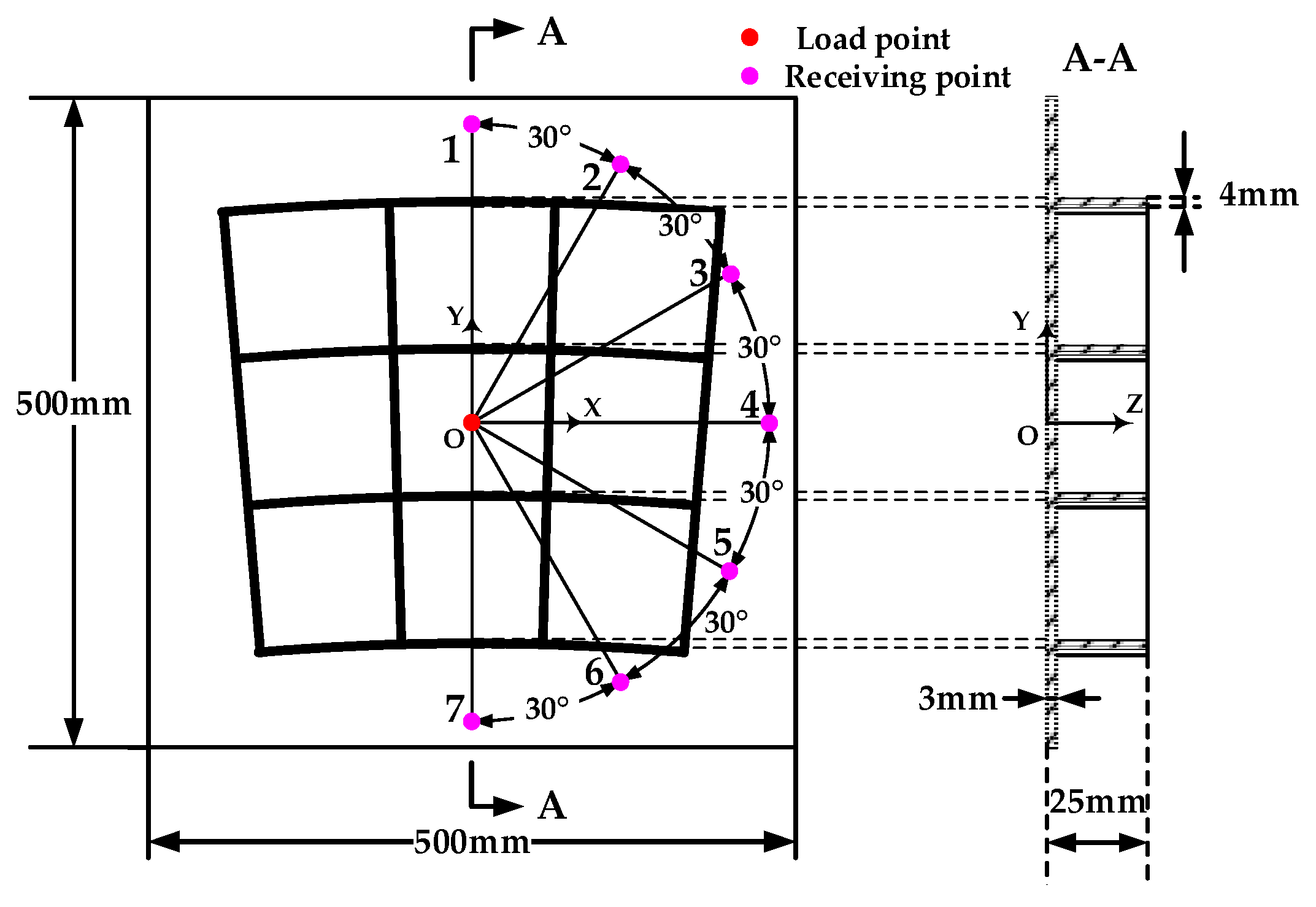
On the flat side of the stiffened panel, the origin is centered, the x-axis is the positive direction, and the counterclockwise is the positive direction. With a radius of 230 mm, a receiving point is set every 30° in the range of −90° to 90°. There are 7 receiving points. The serial number is shown in Figure 4. The straight paths from point 1, point 4 and point 7 to the origin pass through two stiffeners. The straight paths from point 2, point 3, point 5 and point 6 to the origin pass through three stiffeners.
At the same time, in order to eliminate the influence of the propagation distance on the energy attenuation of the Lamb wave, a three-dimensional model of the flat panel with a size of 500 mm × 500 mm × 3 mm is established as a control group, and the parameters and receiving points are set exactly the same as the stiffened panel. Based on the above settings, the established three-dimensional finite element simulation model is shown in Figure 6.
3.2. Effect of Stiffeners on Lamb Wave Velocity and Signal Head
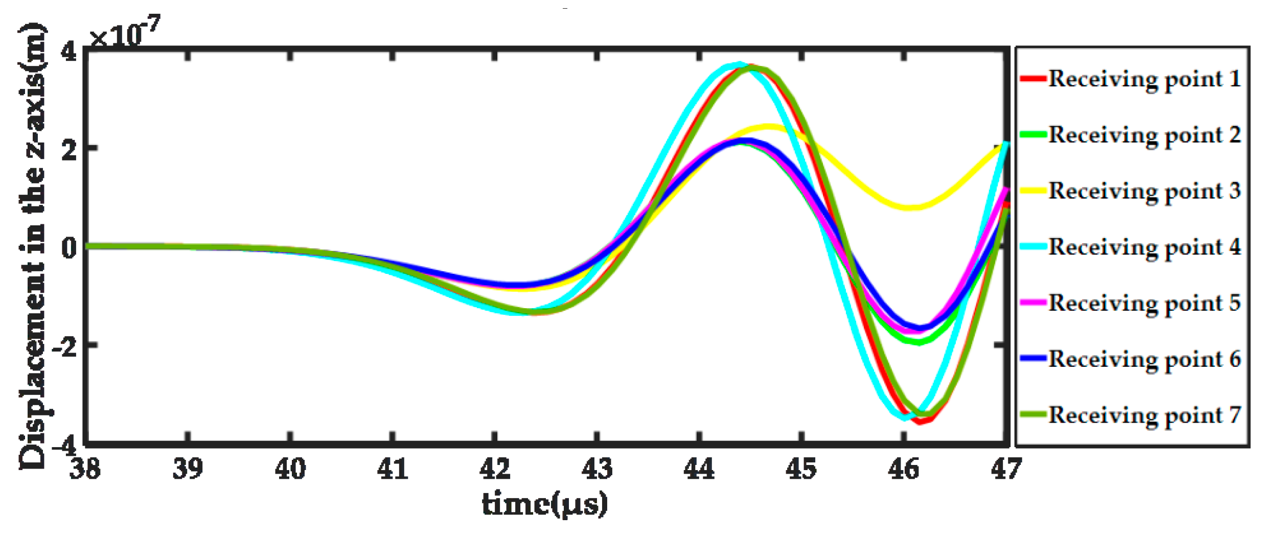
The time-domain waveform of the z-axis displacement obtained at each receiving point of 230 mm from the origin is shown in Figure 7. As can be seen from the figure, the arrival time of the first trough of point 1 to 7 is about 42.2 μs, and the calculated wave velocity is 5.45 km/s. The first wave trough of the Lamb wave after the same number of stiffeners is roughly equal. The first wave trough of the Lamb wave passing through the two stiffeners is significantly higher than passing three stiffeners, which is also applicable to the first wave crest. It can be seen that the number of stiffeners has almost no effect on the Lamb wave velocity. The more stiffeners the signal passes through, the lower the first crest and trough of the signal is.
3.3. Effect of Stiffeners on S0 Mode Lamb Wave
According to the simulation results, the time when the A0 mode Lamb wave reaches the receiving points at 230 mm from the origin is about 70.3 μs, and the S0 mode Lamb wave before 70.3 μs is selected as the research object.
The energy factor curves from point 1 to point 7 at 230 mm from the origin are shown in Figure 8. It can be seen from the figure that the stiffeners have a comb filter effect on the Lamb wave, that is, the Lamb wave energy fluctuates with the change of the frequency. When the number of stiffeners is 2, the comb filter has a clear pass band in the 70 kHz–170 kHz, and the pass band bandwidth is narrow in the 50–100 kHz. The maximum energy factors are in the range of 40–55. As the frequency increases below 300 kHz, the energy factor changes sharply. When the frequency is more than 350 kHz, the energy factors fluctuate only within 0–3. The Lamb wave energy is generally attenuated after passing through the stiffener, but the energy of S0 mode is very small relative to that of A0 mode. When passing through the stiffener, part of A0 mode energy will transfer to S0 mode, which results in that the energy of S0 mode in stiffened panel is much higher than that of S0 mode in panel, so there will be a large energy factor in some frequency bands. When the number of stiffeners is 3, the overall change of the energy factor is gentle. In the 50–250 kHz band, the comb filter has smaller passband and wider bandwidth. The energy factor is also extremely small when the frequency is more than 350 kHz.
Combining the energy factor curves, it can be seen that the energy of S0 mode varies greatly in the frequency band of 50–100 kHz after different number of stiffeners, there is instability. At the same time, the frequency of this band is relatively low and the resolution is not high in the time domain. In practice, the impact signal is a broadband Lamb wave, and the path from the impact source to each sensor is uncertain. The frequency components of Lamb wave received by different sensors are usually quite different. There is a risk of intercepting signals of different frequency bands and different phases at the arrival time of signals obtained by threshold method. At this time, a large error may occur when the locating calculation is performed using the same wave velocity. Based on the above factors, the S0 mode signal characteristics in the 100–200 kHz band meet the locating requirements.
4. Experiments of Impact Source Localization in Stiffened Panel
4.1. Impact Signal Generation and Wave Velocity Measurement
In the impact source locating experiment, the impact source needed to meet the following requirements: the impact source energy must be stable with good repeatability; the impact point position must be precisely controllable; the personnel safety must be ensured. In this paper, a steel projectile is launched by a launcher. The diameter of the projectile was 7.5 mm and the weight was 1.73 g. The initial velocity of the projectile is shown in Table 2. The average velocity was 21.0 m/s.
The wave velocities in 10 directions are measured at intervals of 10° in the range of 0 to 90°. On the flat side of the panel, four sensors were placed at intervals of 100 mm in each direction, with vacuum silicone grease as the couplant. The steel projectile hit the flat side to generate an impact signal, and five experiments were performed in each direction. The Softland Times company’s acoustic emission instrument (DS2-16B) was used to collect data at a sampling rate of 3 MHz, and the receiving sensor was nano 30 produced by the PAC company. The diagram of the experiment is shown in Figure 9.
When calculating the velocity in a certain direction, the signal arrival time of each sensor was obtained by artificially setting the threshold interception waveform, and the velocity was obtained by dividing the distance between two adjacent sensors by the arrival time difference of the received corresponding signal. The two sets of velocities can be calculated in each direction, and the average of the 10 sets of velocities of the five experiments was taken as the wave velocity in that direction. The average value of the wave velocity in each direction is calculated as shown in Table 3.
It can be seen from the table that the measured wave velocities in each direction was basically the same. The overall average velocity was 5.43 km/s, which coincides with the simulation. The experimental results were slightly slower than the simulation results due to the delay effect of the switching device. Therefore, the wave velocity used for impact source localization was 5.43 km/s.
The impact signal received by the sensor was a broadband signal. For the part whose frequency did not exceed 500 kHz, the sampling rate of 3 MHz was sufficient. But the sampling resolution for the part with higher frequency was low, thereby generating errors such that the calculated wave velocity in each direction was not exactly equal. However, the high-frequency portion of the impact signal had a low energy content, and as the propagation distance increased, the attenuation was severe and the energy was further reduced. At the same time, whether the sampling rate matched the spacing of the sensor directly affected the accuracy of the measurement result. The closer the sensors were, the higher the sampling rate was required [48]. The setting in this paper is reasonable. The distance between the adjacent receiving sensors in the same direction was 100 mm, and the distance was large enough. At this time, the sampling rate was 3 MHz, the difference in arrival time of the received signals of any two sensors in the time domain was sufficiently large and can be clearly identified. For the above two reasons, the wave velocity measurement error was small, and the influence on the locating result can be neglected.
4.2. Experimental System
In this paper, the fan-ring shaped high-stiffened panel of sealed bulkhead of manned spacecraft was taken as the research object. The stiffened panel had fan-shaped stiffeners and a rectangular mounting frame. The specific parameters of the panel and stiffener are shown in Table 4. The actual structure of the stiffened panel is shown as Figure 10.
The schematic diagram of the experimental system is shown in Figure 11, which consists of the acoustic emission instrument (Softland Times-DS2-16B), amplifiers (Softland Times-AE Amplifier), sensors (PAC-nano 30), a projectile launcher and the fan-ring shaped stiffened panel.
The inner diameter was zero in the radial direction, the direction away from the center of the circle was the positive direction, the unit length was 50 mm, the right side of the flat plane side was the circumferential direction 0°, counterclockwise was the positive direction, the unit angle was 1°. The polar coordinate system was established. The three sensors were arranged on the flat side with coordinates S1 (450,29), S2 (100,19) and S3 (450,9) with a maximum distance of 819.6 mm between the sensors. Inside the isosceles triangle formed by the sensors, an impact point was set with the intervals of 50 mm and 2°, for a total of 32 impact points. The distribution of impact points is shown in Figure 12.
The experimental system is shown in Figure 13. During the experiment, the steel projectile was launched at the impact point using the launching device to generate the impact signal in turn, and the experiment was repeated three times per point.
5. Results
5.1. Locating Results without Filtering
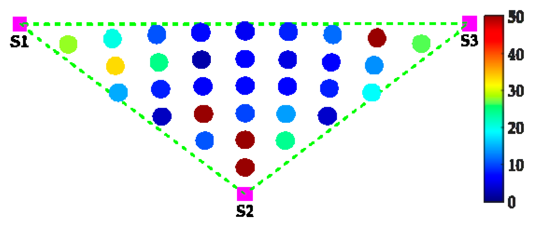
The impact experiment was performed in each of the impact points in Figure 12 in sequence, and the locating was performed by the AECTF method. The coordinates of the impact points were recorded as actual coordinates, and the coordinates calculated by the AECTF method were recorded as calculated coordinates. The linear distance between the real coordinate and the calculated coordinate was taken as absolute error, and the ratio of absolute error to the maximum side length of the triangle formed by the sensor was taken as relative error. The error average of the three experiments was taken as the final result.
The distribution of absolute errors using the signals without filtering is shown in Figure 14. The color of each point represents the magnitude of absolute error in mm. The results show that among the 32 impact points locating results, except the errors of the impact points near the distance sensor are larger, 27 points errors were less than 30 mm. The proposed algorithm had better locating accuracy and stability.
5.2. Locating Results with Filtering
In order to analyze the influence of the filter bands on the locating results, the impact signals filtered by different frequency bands were used for locating. After the wave velocity measurement signals of Section 3.1 were filtered by different frequency bands, the signal wave velocity of this frequency band was calculated.
The distributions of absolute errors using the signals with 0–100 kHz, 100–200 kHz and 200–300 kHz filtering respectively are shown in Figure 15.
It can be seen from Figure 15 that the locating results after 0–100 kHz filtering fluctuated greatly. Errors of five points were greater than 50 mm, errors of 23 points were less than 30 mm, and the locating stability was not high. For 200–300 kHz filtering, there were three points with errors greater than 50 mm and 27 points with errors less than 30 mm, similar to the unfiltered results. For 100–200 kHz filtering, the maximum error of 32 impact points locating results was only 16.3 mm, the average absolute error of 96 groups of data was 7.0 mm, the average relative error was 0.86%, the error standard deviation was 3.5 mm, the locating accuracy was high and the stability was good, which verifies the correctness of the simulation.
For the impact points near the center of the sensor triangle, various methods can obtain better locating results. However, it was relatively difficult to locate the impact points near the triangle boundary, especially the points near the vertex. In order to further analyze the cause of the locating error, the time domain waveform of a group of experimental signals in the impact experiment at point D1 (in Figure 12) was taken as the research object, and the arrival time of the signal calculated by each method was compared with the actual arrival time.
The comparison of the calculated arrival time and the actual arrival time of the signals with different frequency bands filtering is shown in Figure 16. It can be seen from the figure that the error was mainly caused by two reasons: (1) the noise was complicated before the S0 mode arrived, and the threshold intercepted the noise signal; (2) The threshold was so large that it skipped the head of S0 mode.
This is mainly because the situations of passing through the stiffeners greatly differed in which impact signal at the point D1 propagated to sensors, which made the signals received by the sensors greatly different in the time domain and the frequency domain. The S0 mode filtered in the 100–200 kHz band had the relatively clearer head, which was easier to distinguish from noise. The threshold obtained by the AECTF method based on the energy compensation can truly reflect the signal characteristics, and adaptively intercepts the arrival time of the S0 mode, thereby achieving correct locating.
5.3. Locating Results with Fixed Parameter
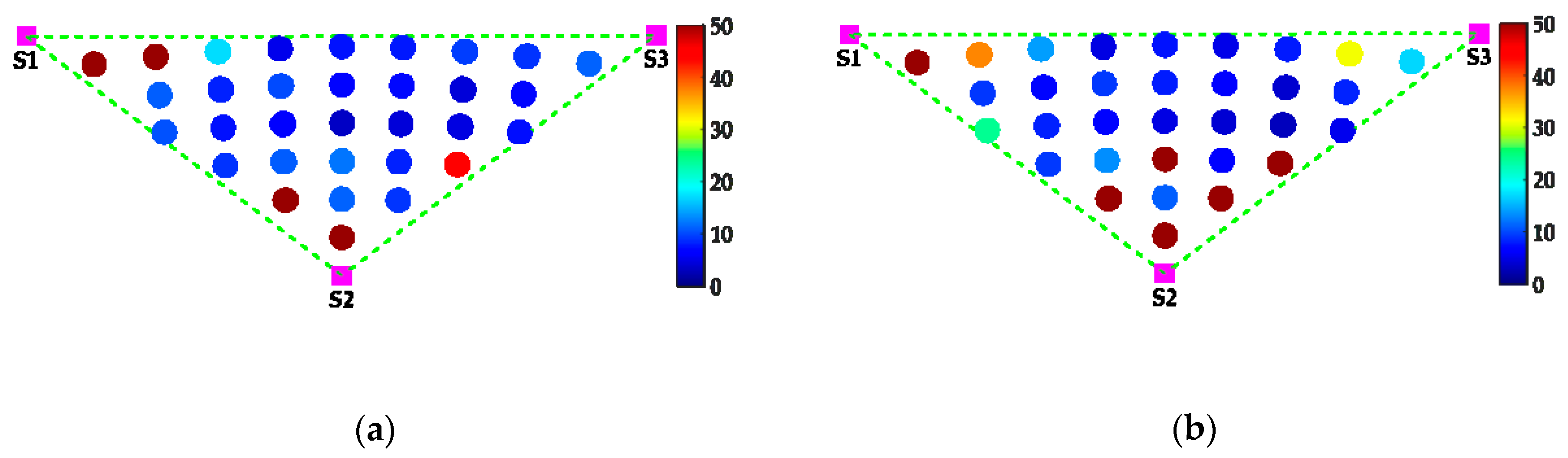
In order to verify the self-adaptability of the AECTF method, the impact signal was filtered by a 100–200 kHz band. Then the signal arrival time was obtained by using the fixed threshold amplification factor and the fixed threshold respectively. The distribution of absolute errors using the fixed parameters is shown in Figure 17. It can be seen from the figure that the locating results had large error points, whether based on fixed threshold amplification factor or fixed threshold.
The comparison of locating errors with different processing methods is shown in Table 5. It can be seen that the locating results have higher accuracy and stability when located by AECTF method.
6. Conclusions
This paper proposes an AECTF method that solves the problem of large-scale accurate and fast localization of impact sources in a high-stiffened panel. The influence of the stiffeners on the Lamb wave is studied. The impact location test is carried out in a fan-ring shaped stiffened panel of sealed bulkhead of manned spacecraft with stiffeners height of 22 mm and the locating was carried out. The results show:
- (1)
- The stiffener has almost no influence on the Lamb wave velocity, and the average wave velocity in each direction can be used as the impact locating wave velocity. When the Lamb wave passes through the same number of stiffeners, the amplitude of the first wave trough is basically the same. The more stiffeners the signal passes through, the more obvious the attenuation of the first wave trough is, and the same applies to the first wave crest.
- (2)
- The stiffener has a comb-filter effect on the S0 mode Lamb wave, and the number of passbands, the bandwidth and fluctuation of filter are related to the through-stiffener condition. When the number of stiffeners is two, there is a clear pass band in the 70–170 kHz band, the pass band bandwidth is narrow, below 100 kHz. When the number of stiffeners is 3, the energy factor changes gently, and a wide pass band exists when the frequency is lower than 250 kHz. Comprehensive energy factor and frequency characteristics, the energy of the 100–200 kHz band signal is relatively high, and the time domain resolution is high, which is suitable for locating.
- (3)
- The AECTF method proposed in this paper has high locating accuracy and stability. When the signal is not filtered, the average locating errors of 84.4% impact points are less than 30 mm. Selecting the appropriate frequency band to filter the impact signals can further improve the locating results. The locating result is optimal when using 100–200 kHz band filtering. The maximum absolute error of 32 points is 16.3 mm, the average absolute error is 7.0 mm, the average relative error is 0.86% and the error standard deviation is 3.5 mm. There are large error points in the locating results of fixed threshold amplification factor and fixed threshold. By comparing the calculated arrival time and the actual arrival time of the signals, it is known that if the threshold is too small, it will be intercepted by noise. If the threshold is too large, the threshold will skip the S0 mode head. The AECTF method can adaptively acquire the arrival time of the S0 mode.
Author Contributions
Y.L. and Z.W. established the finite element model and performed the simulation; Z.W., X.R., L.Q. and Y.L. designed the experiments; L.Q., Z.W. and J.L. performed the experiment; X.R., Z.W. and Z.Y. analyzed the data. All authors reviewed the manuscript.
Funding
This research was funded by National Key R&D Program of China (No. 2018YFF0212201), Natural Science Foundation of Tianjin (No. 17JCYBJC19300) and State Key Laboratory of Precision Measurement Technology and Instrument Fund (Pilab-1706).
Conflicts of Interest
The authors declare no conflict of interest.
References
- Shan, M.H.; Guo, J.; Gill, E. Review and comparison of active space debris capturing and removal methods. Prog. Aerosp. Sci. 2016, 80, 18–32. [Google Scholar] [CrossRef]
- Schildknecht, T. Optical surveys for space debris. Astron. Astrophys. Rev. 2007, 14, 41–111. [Google Scholar] [CrossRef]
- Wright, D. Space debris. Phys. Today 2007, 60, 35–40. [Google Scholar] [CrossRef]
- Valk, S.; Lemaitre, A.; Deleflie, F. Semi-analytical theory of mean orbital motion for geosynchronous space debris under gravitational influence. Adv. Space Res. 2009, 43, 1070–1082. [Google Scholar] [CrossRef]
- Valk, S.; Lemaitre, A.; Anselmo, L. Analytical and semi-analytical investigations of geosynchronous space debris with high area-to-mass ratios. Adv. Space Res. 2008, 41, 1077–1090. [Google Scholar] [CrossRef]
- Liou, J.C.; Johnson, N.L. Planetary science - Risks in space from orbiting debris. Science 2006, 311, 340–341. [Google Scholar] [CrossRef]
- Liu, Z.D.; Pang, B.J. A method based on acoustic emission for locating debris cloud impact. In Proceedings of the 4th International Conference on Experimental Mechanics, Singapore, 18–20 November 2009. [Google Scholar]
- Xie, W.H.; Meng, S.H.; Ding, L.; Jin, H.; Du, S.Y.; Han, G.K.; Wang, L.B.; Xu, C.H.; Scarpa, F.; Chi, R.Q. High-temperature high-velocity impact on honeycomb sandwich panels. Compos. Part B-Eng. 2018, 138, 1–11. [Google Scholar] [CrossRef] [Green Version]
- Zhang, Z.Y.; Chi, R.Q.; Pang, B.J.; Guan, G.S. Numerical simulation of projectile oblique impact on microspacecraft structure. Int. J. Aerosp. Eng. 2017. Available online: https://www.hindawi.com/journals/ijae/2017/1015674/ (accessed on 28 April 2019). [CrossRef]
- Schaub, H.; Jasper, L.E.Z.; Anderson, P.V.; McKnight, D.S. Cost and risk assessment for spacecraft operation decisions caused by the spacedebris environment. Acta Astronaut. 2015, 113, 66–79. [Google Scholar] [CrossRef]
- Grossman, E.; Gouzman, I.; Verker, R. Debris/Micrometeoroid impacts and synergistic effects on spacecraft materials. MRS Bull. 2010, 35, 41–47. [Google Scholar] [CrossRef]
- Tommei, G.; Milani, A.; Rossi, A. Orbit determination of space debris: Admissible regions. Celest. Mech. Dyn. Astr. 2007, 97, 289–304. [Google Scholar] [CrossRef]
- Alby, F.; Lansard, E.; Michal, T. Collision of cerise with space debris. In Proceedings of the 2nd European Conference on Space Debris, ESOC, Darmstadt, Germany, 17–19 March 1997; p. 589. [Google Scholar]
- Golub, M.V.; Shpak, A.N. Semi-analytical hybrid approach for the simulation of layered waveguide with a partially debonded piezoelectric structure. Appl. Math. Model. 2019, 65, 234–255. [Google Scholar] [CrossRef]
- Reusser, R.S.; Chimenti, D.E.; Roberts, R.A.; Holland, S.D. Guided plate wave scattering at vertical stiffeners and its effect on source location. Ultrasonics 2012, 52, 687–693. [Google Scholar] [CrossRef]
- Reusser, R.S.; Holland, S.D.; Chimenti, D.E.; Roberts, R.A. Reflection and transmission of guided ultrasonic plate waves by vertical stiffeners. J. Acoust. Soc. Am. 2014, 136, 170–182. [Google Scholar] [CrossRef] [PubMed]
- Ghandourah, E. Large Plate Monitoring Using Guided Ultrasonic Waves. Ph.D. Thesis, University College London, London, UK, 2015. Available online: http://discovery.ucl.ac.uk/1463979/ (accessed on 28 April 2019).
- Santhanam, S.; Demirli, R. Reflection of lamb waves obliquely incident on the free edge of a plate. Ultrasonics 2013, 53, 271–282. [Google Scholar] [CrossRef] [PubMed]
- Haider, M.F.; Bhuiyan, M.Y.; Poddar, B.; Lin, B.; Giurgiutiu, V. Analytical and experimental investigation of the interaction of Lamb waves in a stiffened aluminum plate with a horizontal crack at the root of the stiffener. J. Sound Vib. 2018, 431, 212–225. [Google Scholar] [CrossRef]
- Alleyne, D.N.; Cawley, P. The interaction of Lamb waves with defects. IEEE Trans. Ultrason. Ferroelectr. 1992, 39, 381–397. [Google Scholar] [CrossRef] [PubMed]
- Benmeddour, F.; Grondel, S.; Assaad, J.; Moulin, E. Study of the fundamental Lamb modes interaction with asymmetrical discontinuities. NDT&E Int. 2008, 41, 330–340. [Google Scholar]
- Tuzzolino, A.J.; McKibben, R.B.; Simpson, J.A.; BenZvi, S.; Voss, H.D.; Gursky, H. The Space Dust (SPADUS) instrument aboard the Earth-orbiting ARGOS spacecraft: I—instrument description. Planet. Space Sci. 2001, 49, 689–703. [Google Scholar] [CrossRef]
- Tuzzolino, A.J.; McKibben, R.B.; Simpson, J.A.; BenZvi, S.; Voss, H.D.; Gursky, H. The Space Dust (SPADUS) instrument aboard the Earth-orbiting ARGOS spacecraft: II- results from the first 16 months of flight. Planet. Space Sci. 2001, 49, 705–729. [Google Scholar] [CrossRef]
- Jia, Z.G.; Ren, L.; Li, H.N.; Sun, W. Pipeline leak localization based on FBG hoop strain sensors combined with BP neural network. Appl. Sci. 2018, 8, 146. [Google Scholar] [CrossRef]
- Rickman, S.L.; Richards, W.L.; Christiansen, E.L.; Piazza, A.; Pena, F.; Parker, A.R. Micrometeoroid/orbital debris (MMOD) impact detection and location using fiber optic bragg grating sensing technology. Procedia Eng. 2017, 188, 233–240. [Google Scholar] [CrossRef]
- Yeager, M.; Whittaker, A.; Todd, M.; Kim, H.; Key, C.; Gregory, W. Impact detection and characterization in composite laminates with embedded fiber Bragg gratings. In Proceedings of the 6th Asia-Pacific Workshop on Structural Health Monitoring (APWSHM), Hobart, Australia, 7–9 December 2016; pp. 156–162. [Google Scholar]
- Ongpeng, J.M.C.; Oreta, A.W.C.; Hirose, S. Monitoring damage using acoustic emission source location and computational geometry in reinforced concrete beams. Appl. Sci. 2018, 8, 189. [Google Scholar] [CrossRef]
- Bartoli, I.; Salamone, S.; di Scalea, F.L.; Rhymer, J.; Kim, H. Impact force identification in aerospace panels by an inverse ultrasonic guided wave problem. In Proceedings of the Conference on Health Monitoring of Structural and Biological Systems 2011, San Diego, CA, USA, 7–10 March 2011. [Google Scholar]
- Zhou, Z.L.; Rui, Y.C.; Zhou, J.; Dong, L.J.; Chen, L.J.; Cai, X.; Cheng, R.S. A new closed-form solution for acoustic emission source location in the presence of outliers. Appl. Sci. 2018, 8, 949. [Google Scholar] [CrossRef]
- Salamone, S.; Bartoli, I.; Rhymer, J.; di Scalea, F.L.; Kim, H. Validation of the piezoelectric rosette technique for locating impacts in complex aerospace panels. In Proceedings of the Conference on Health Monitoring of Structural and Biological Systems 2011, San Diego, CA, USA, 7–10 March 2011. [Google Scholar]
- Wu, J.C.; Xu, C.H.; Qi, B.X.; Hernandez, F.C.R. Detection of impact damage on PVA-ECC beam using infrared thermography. Appl. Sci. 2018, 8, 839. [Google Scholar] [CrossRef]
- Liu, Z.H.; Wang, J.M.; Kong, F.J.; Liu, W.G.; Li, H.B. A method for locating space debris impact source based on PVDF films. In Proceedings of the 11th International Space Conference on Protection of Materials and Structures from Space Environment (ICPMSE), Lijiang, China, 19–23 May 2014; pp. 509–515. [Google Scholar]
- Qi, B.X.; Kong, Q.Z.; Qian, H.; Patil, D.; Lim, I.; Li, M.; Liu, D.; Song, G.B. Study of impact damage in PVA-ECC beam under low-velocity impact loading using piezoceramic transducers and PVDF thin-film transducers. Sensors 2018, 18, 671. [Google Scholar] [CrossRef] [PubMed]
- Han, J.; Li, D.; Zhao, C.M.; Wang, X.Y.; Li, J.; Wu, X.Z. Highly sensitive impact sensor based on PVDF-TrFE/Nano-ZnO composite thin film. Sensors 2019, 19, 830. [Google Scholar] [CrossRef]
- Shrestha, P.; Kim, J.H.; Park, Y.; Kim, C.G. Impact localization on composite structure using FBG sensors and novel impact localization technique based on error outliers. Compos. Struct. 2016, 142, 263–271. [Google Scholar] [CrossRef]
- Wang, J.K.; Huo, L.S.; Liu, C.G.; Peng, Y.C.; Song, G.B. Feasibility study of real-time monitoring of pin connection wear using acoustic emission. Appl. Sci. 2018, 8, 1775. [Google Scholar] [CrossRef]
- Sanchez, N.; Meryane, V.; Ortiz-Bernardin, A. A novel impact identification algorithm based on a linear approximation with maximum entropy. Smart Mater. Struct. 2016, 25, 095050. [Google Scholar] [CrossRef]
- Zhang, L.; Ozevin, D.; He, D.; Hardman, W.; Timmons, A. A method to decompose the streamed acoustic emission signals for detecting embedded fatigue crack signals. Appl. Sci. 2018, 8, 7. [Google Scholar] [CrossRef]
- Meruane, V.; Veliz, P.; Droguett, E.L.; Ortiz-Bernardin, A. Impact location and quantification on an aluminum sandwich panel using principal component analysis and linear approximation with maximum entropy. Entropy 2017, 19, 137. [Google Scholar] [CrossRef]
- Teng, X.D.; Zhang, X.; Fan, Y.T.; Zhang, D. Evaluation of cracks in metallic material using a self-organized data-driven model of acoustic echo-signal. Appl. Sci. 2019, 9, 95. [Google Scholar] [CrossRef]
- Chen, C.L.; Li, Y.L.; Yuan, F.G. Impact source identification in finite isotropic plates using a time-reversal method: experimental study. Smart Mater. Struct. 2012, 21, 105025. [Google Scholar] [CrossRef]
- Salmanpour, M.S.; Khodaei, Z.S.; Aliabadi, M.H. Transducer placement optimisation scheme for a delay and sum damage detection algorithm. Struct. Control Health 2017, 24, e1898. [Google Scholar] [CrossRef]
- Park, W.H.; Packo, P.; Kundu, T. Acoustic source localization in an anisotropic plate without knowing its material properties—A new approach. Ultrasonics 2017, 79, 9–17. [Google Scholar] [CrossRef]
- Sen, N.; Kundu, T. A new wave front shape-based approach for acoustic source localization in an anisotropic plate without knowing its material properties. Ultrasonics 2018, 87, 20–32. [Google Scholar] [CrossRef]
- Marino-Merlo, E.; Bulletti, A.; Giannelli, P.; Calzolai, M.; Capineri, L. Analysis of errors in the estimation of impact positions in plate-like structure through the triangulation formula by piezoelectric sensors monitoring. Sensors 2018, 18, 3426. [Google Scholar] [CrossRef]
- Jiao, J.P.; Meng, X.J.; He, C.F.; Bin, W. Nonlinear Lamb wave-mixing technique for micro-crack detection in plates. NDT&E Int. 2017, 85, 63–71. [Google Scholar]
- Moreau, L.; Velichko, A.; Wilcox, P.D. Accurate finite element modelling of guided wave scattering from irregular defects. NDT&E Int. 2012, 45, 46–54. [Google Scholar]
- Maio, L.; Ricci, F.; Memmolo, V.; Monaco, E.; Boffa, N.D. Application of laser Doppler vibrometry for ultrasonic velocity assessment in a composite panel with defect. Compos. Struct. 2018, 184, 1030–1039. [Google Scholar] [CrossRef]
Figure 1.
Flow chart of the adaptive energy compensation threshold filtering (AECTF) method.

Figure 2.
Dispersion curves for 3 mm-thick 5A06 aluminum plate: (a) phase velocity; (b) group velocity.
Figure 2.
Dispersion curves for 3 mm-thick 5A06 aluminum plate: (a) phase velocity; (b) group velocity.
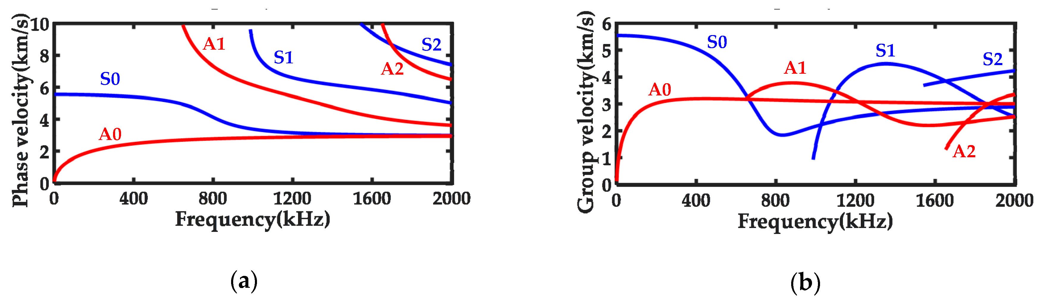
Figure 3.
Locating principle diagram.

Figure 4.
The schematic diagram of model (absorbing layers are not shown).

Figure 5.
Load characteristics: (a) time domain; (b) frequency domain.

Figure 6.
Three-dimensional finite element simulation model: (a) stiffened panel; (b) flat panel.
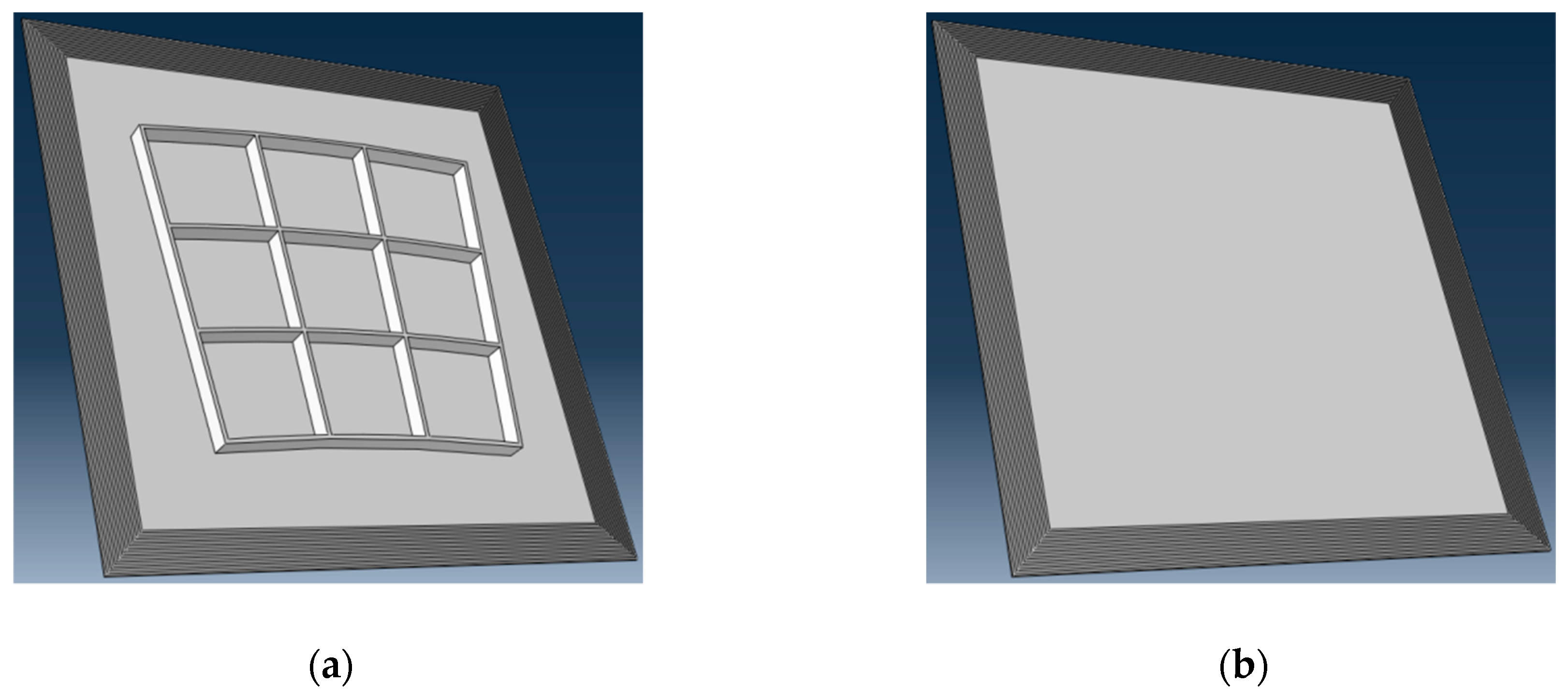
Figure 7.
Displacement in the z-axis of each receiving point.

Figure 8.
Energy factor curves: (a) point 1; (b) point 2; (c) point 3; (d) point 4; (e) point 5; (f) point 6; (g) point 7.
Figure 8.
Energy factor curves: (a) point 1; (b) point 2; (c) point 3; (d) point 4; (e) point 5; (f) point 6; (g) point 7.


Figure 9.
The schematic diagram of wave velocity measurement experiment.

Figure 10.
The fan-ring shaped high-stiffened panel actual structure diagram: (a) flat side; (b) stiffened side.
Figure 10.
The fan-ring shaped high-stiffened panel actual structure diagram: (a) flat side; (b) stiffened side.
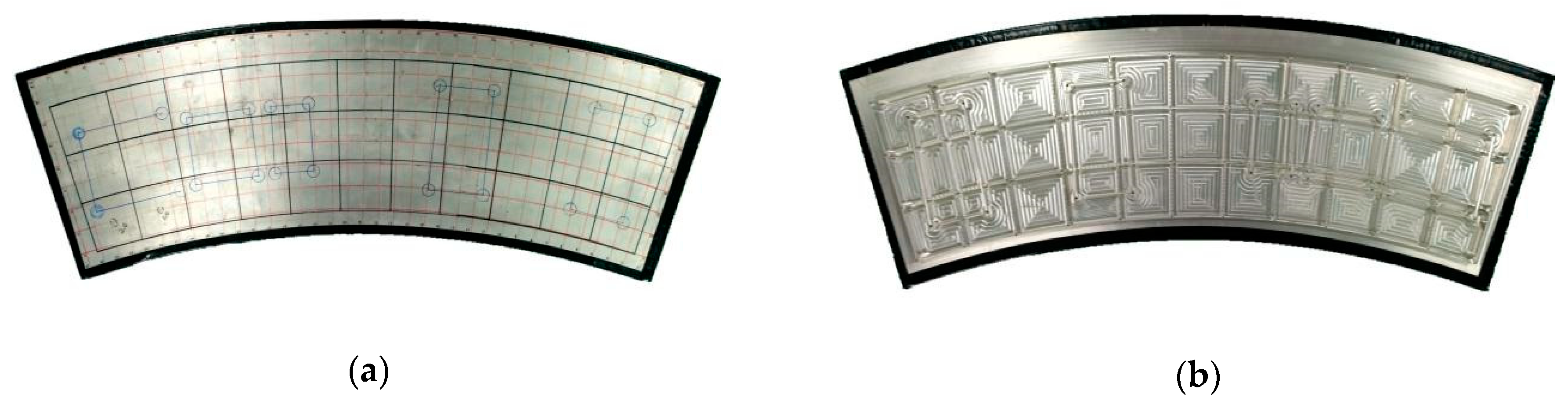
Figure 11.
The schematic diagram of the experimental system.

Figure 12.
The distribution of impact points.

Figure 13.
Experimental system.
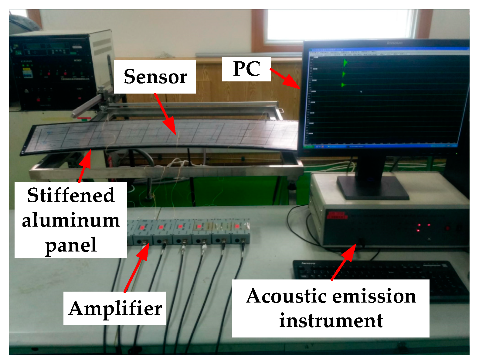
Figure 14.
The distribution of absolute errors using the signals without filtering.

Figure 15.
The distributions of absolute errors using the signals with different frequency bands filtering: (a) 0–100 kHz; (b) 100–200 kHz; (c) 200–300 kHz.
Figure 15.
The distributions of absolute errors using the signals with different frequency bands filtering: (a) 0–100 kHz; (b) 100–200 kHz; (c) 200–300 kHz.

Figure 16.
The comparison of the calculated arrival time and the actual arrival time of the signals with different frequency bands filtering: (a) signals of sensors 1–3 without filtering; (b) signals of sensors 1–3 with 0–100 kHz filtering; (c) signals of sensors 1–3 with 100–200 kHz filtering; (d) signals of sensors 1–3 with 200–300 kHz filtering.
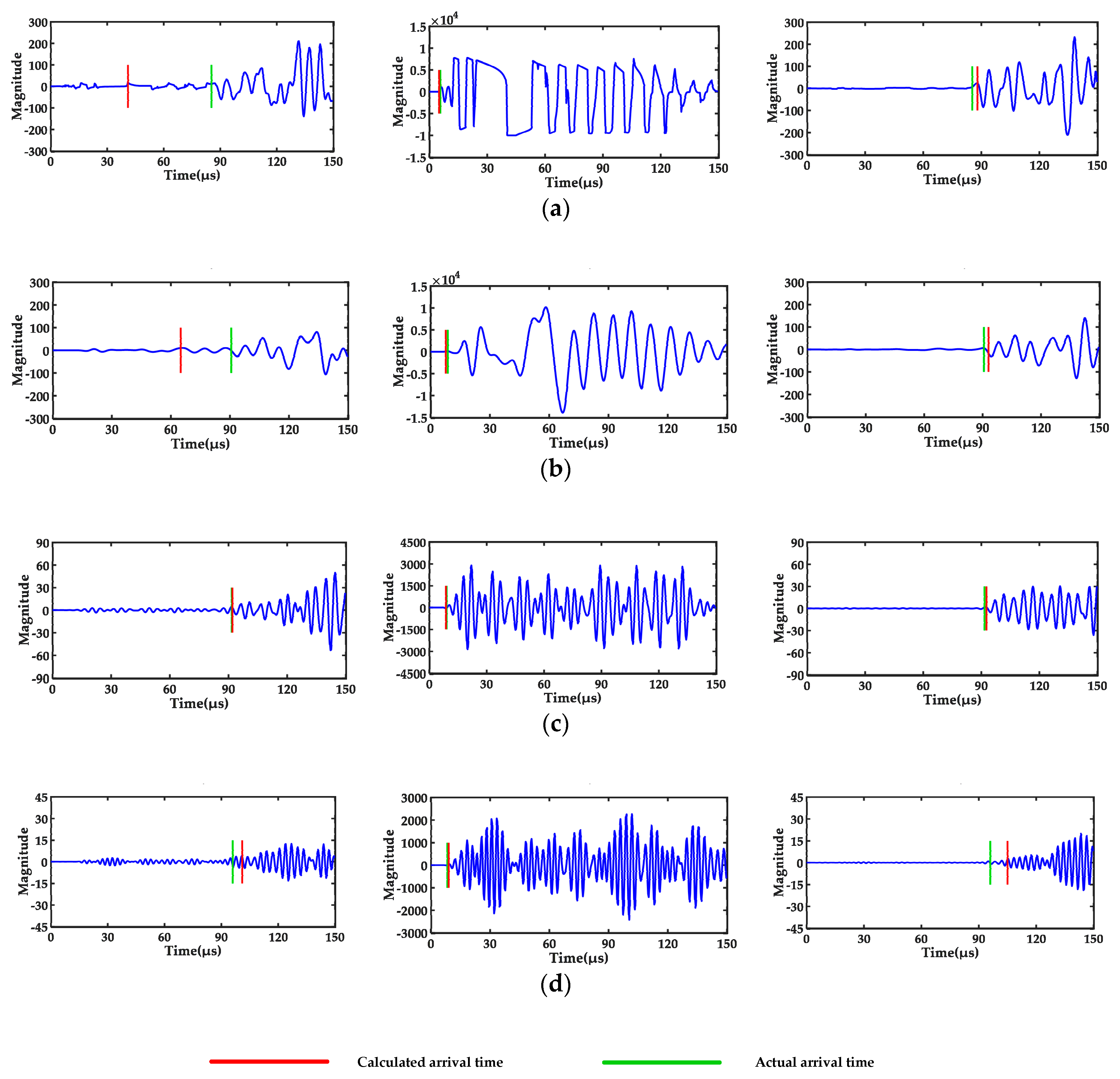
Figure 17.
The distribution of absolute errors using the fixed parameters: (a) fixed threshold amplification factor; (b) fixed threshold.
Figure 17.
The distribution of absolute errors using the fixed parameters: (a) fixed threshold amplification factor; (b) fixed threshold.

Table 1.
The material parameters of the stiffened panel.
| Aluminum Designation | ρ (g/cm3) | E (MPa) | μ |
|---|---|---|---|
| 5A06 | 2.64 | 71,000 | 0.32 |
Table 2.
Steel projectile initial velocity.
| Number of experiments | 1 | 2 | 3 | 4 | 5 | 6 | 7 | 8 | 9 | 10 |
| Velocity (m/s) | 21.3 | 21.4 | 21.4 | 20.9 | 21.2 | 21.3 | 19.4 | 21.1 | 21.3 | 20.9 |
Table 3.
Average wave velocity in each direction.
| Angle (°) | 0 | 10 | 20 | 30 | 40 | 50 | 60 | 70 | 80 | 90 |
| Wave velocity (km/s) | 5.43 | 5.46 | 5.47 | 5.42 | 5.40 | 5.45 | 5.41 | 5.43 | 5.46 | 5.40 |
Table 4.
The parameters of the fan-ring shaped high-stiffened panel.
| Dimension Parameter | Value | Dimension Parameter | Value |
|---|---|---|---|
| Outer diameter (mm) | 2378.8 | Height of stiffener (mm) | 22.0 |
| Inner diameter (mm) | 1910.0 | Thickness of stiffener (mm) | 4.0 |
| Central angle (°) | 37.8 | Circumferential spacing (°) | 3.2 |
| Width (mm) | 468.8 | Radial spacing (mm) | 112.0 |
| Thickness (mm) | 3.0 | Material | Aluminum 5A06 |
Table 5.
The comparison of locating errors under different processing methods.
| Different Processing Methods | Average Absolute Error (mm) | Average Relative Error | Error Standard Deviation (mm) |
|---|---|---|---|
| Without filtering | 25.4 | 3.10% | 38.2 |
| With 0–100 kHz filtering | 28.6 | 3.49% | 29.7 |
| With 100–200 kHz filtering | 7.0 | 0.86% | 3.5 |
| With 200–300 kHz filtering | 19.9 | 2.43% | 18.8 |
| Fixed threshold amplification factor with 100–200 kHz filtering | 17.5 | 2.13% | 23.1 |
| Fixed threshold with 100–200 kHz filtering | 27.8 | 3.39% | 41.0 |
© 2019 by the authors. Licensee MDPI, Basel, Switzerland. This article is an open access article distributed under the terms and conditions of the Creative Commons Attribution (CC BY) license (http://creativecommons.org/licenses/by/4.0/).
Share and Cite
MDPI and ACS Style
Li, Y.; Wang, Z.; Rui, X.; Qi, L.; Liu, J.; Yang, Z. Impact Location on a Fan-Ring Shaped High-Stiffened Panel Using Adaptive Energy Compensation Threshold Filtering Method. Appl. Sci. 2019, 9, 1763. https://doi.org/10.3390/app9091763
AMA Style
Li Y, Wang Z, Rui X, Qi L, Liu J, Yang Z. Impact Location on a Fan-Ring Shaped High-Stiffened Panel Using Adaptive Energy Compensation Threshold Filtering Method. Applied Sciences. 2019; 9(9):1763. https://doi.org/10.3390/app9091763
Chicago/Turabian StyleLi, Yibo, Zhe Wang, Xiaobo Rui, Lei Qi, Jiawei Liu, and Zi Yang. 2019. "Impact Location on a Fan-Ring Shaped High-Stiffened Panel Using Adaptive Energy Compensation Threshold Filtering Method" Applied Sciences 9, no. 9: 1763. https://doi.org/10.3390/app9091763
Note that from the first issue of 2016, this journal uses article numbers instead of page numbers. See further details here.