Establishing a Risk Profile for New Zealand Pastoral Farms


1
Agriculture and Horticulture, Massey University, Palmerston North 4410, New Zealand
2
Ravensdown Ltd., Hornby, Christchurch 8140, New Zealand
*
Author to whom correspondence should be addressed.
Agriculture 2017, 7(10), 81; https://doi.org/10.3390/agriculture7100081
Submission received: 5 September 2017
/
Revised: 19 September 2017
/
Accepted: 19 September 2017
/
Published: 22 September 2017
Abstract
:In this paper, the risk profile of two pastoral production systems in New Zealand are examined. All farmers must manage and mitigate a multitude of risks. Traditionally, a farm budget is solely undertaken to satisfy a lending institution. Limited variance analysis takes place, usually for output prices and inputs such as: interest rates, energy costs, and fertiliser. The authors of this paper use “@Risk”, a risk profiling plug-in tool for Microsoft Excel to demonstrate how farm budgets can be more relevant to farmers. Many risk factors that affect farm financial performance, such as climate and commodity prices, are not controlled by the farmer. Wet summers help hill country sheep and beef pastoral farmers, as more grass growth occurs, which thereby reduces the cost of production and increases revenue, as more stock is finished. Whereas in drought years income falls as stock must be sold prior to finishing, in severe droughts capital stock may also be sold. Input costs also rise as pasture weed invasion occurs; health issues such as rye grass staggers may also add cost. Monte Carlo simulations on model farm budgets for a North Island sheep and beef property and a Canterbury dairy farm help demonstrate the risk profile of each farm type.
1. Introduction
This commentary uses risk profiling software on a model dairy farm and a hard, steep hill country sheep and beef property in New Zealand. The authors demonstrate the method based on their experience working in the agricultural sector for over thirty years. Risk profiling is not an exact science; it provides a range of outcomes with a probability based upon the parameters of the frequency distributions fitted. In this work, two sets of financial budgets generated from industry data are used as inputs to provide examples of risk profiles. The methods employed could be of benefit to pastoral farmers in New Zealand.
Farm production systems provide financial opportunity but are fraught with risk. Some farmers may experience greater than average profit margins, whilst others experience a total crop loss even if they are using similar production systems. Misfortune to producers in one region can reduce supply and increase the price received by unaffected producers of the same commodity in another region.
Farmers run businesses and must manage and mitigate risk. Many factors that generate financial risk are not able to be controlled by the farmer [1,2]. For some farmers, risk mitigation is possible. Irrigation, for example, can reduce risks associated with drought. Two farms are risk profiled by the authors: one a sheep and beef farm which is not irrigated, whereas the dairy farm modelled is irrigated. Although specific event insurance may be purchased to reduce the risk of a large reduction of income, this is more common in horticulture and arable situations (e.g., hail cover) [1].
When making business decisions and investment choices some partial budgeting and variance analysis is undertaken in order to rank opportunities and assess risk. Risk profiling as an additional tool to variance analysis is ideal for agricultural systems. This commentary demonstrates how risk profiling can be undertaken on two pastoral farming systems and how it may be used to assist farmers in their decision making.
The risks of an agricultural production system can be modelled by a frequency distribution. Palisade “@Risk” (Palisade, Ithaca, NY) provides a large range of distributions which may be fitted to spreadsheet inputs; for this exercise, they are fitted to typical farm budgets of a sheep and beef and dairy farm. For the sheep and beef farm a “normal distribution” is fitted to annual rainfall based on the 30-year average [3]. The “normal distribution” is fitted to most of the natural systems for this simulation exercise. Consider, for example, that the numbers of lambs survived will vary depending on weather at lambing, but will always be less than average in a cold, wet spring than a mild one. The proportion of calves born that are female is more or less 0.5. The farm gate commodity price achieved is far more variable than the natural systems that drive production. There tends to be an inflationary trend increase to prices achieved, the trend is weak and for this exercise a risk profile is built for a specific budget covering a 12-month period [4].
The analyst has a large selection of distributions which may be applied to inputs. A commodity may be at a record low price and an input for the commodity price may be chosen with a positive skew, as the analyst may expect the price to increase or vice versa. As each simulation takes a few seconds, any number of situations could be considered. For the examples demonstrated in this commentary, the current price for livestock was used with a “normal distribution”. A price of $6.00 per kg milk solids (kg MS−1) was used in the dairy farm, although the current price is $6.50, as this was the price used in [5,6]. The standard deviation for any distribution is defined by the user, and, for this exercise, they were set to reflect deviation in price movements over recent years.
Rainfall for hill country sheep and beef farms is positively correlated to price achieved for stock sold, and negatively correlated to cost of stock feed. This is because when rainfall (especially summer rainfall) is higher than average stock can be finished cheaply on farm, as pasture remains actively growing and is the cheapest means of feeding stock. Wetter summers also mean that more grass can be harvested as hay and baleage, which provides more stock feed options, thus increasing the supply of stock feed supplements and reducing the demand and price of all feed supplements and grains fed to dairy cattle. The inverse occurs in times of drought, when stock must be sold early and cheaply and feed may need to be brought in to support capital livestock. Whereas for the dairy farm, which is irrigated, the price achieved for milk solid is highly variable, and has a high standard deviation [2,4,5,6]. Distributions can be either continuous, for variation in income output, or discrete, for example, the number of cows as in the stock numbers used in this commentary. Many costs such as repairs and maintenance should be fitted with positively skewed distributions, as there is a possibility of the costs being under budget, although they are usually close to budget if they are less than those budgeted. However, these costs have a chance of a large budget blowout. These situations occur from natural disasters, such as occasional floods and storms.
Once the distributions are fitted to the inputs and correlations established, a simulation may be run and the resulting effects on the selected outputs found. Outputs are items of interest such as total revenue, grouped expenses, and profit. The software is capable of 2 billion random sampling iterations of the Monte Carlo simulations to provide a system risk profile.
2. Methods
The method chosen to demonstrate risk profiling is by case study. Case studies are undertaken on farm budgets as they are common to all farmers and presented in a similar format as those presented here. Farm benchmarking data was used to build a hypothetical set of accounts created for a 4033 ha sheep station in the lower Western North island of New Zealand (LWNI), which provides publicly available information via a website [7,8]. Similarly, a model dairy farm benchmarking financial analysis was found for a Canterbury dairy farm [9]. This dairy model farm budget was used as it was developed when the milk solid farm gate price was $8.54 kg−1, the budget price was $6.00 kg−1, whilst the actual 2014/2015 price was $4.71 kg−1, the 2015/2016 price was $4.30 kg−1, and the current price is $6.50 kg−1. Normal frequency distributions were fitted based on the authors’ judgement of commodity price movements of milk solids, cow beef, lamb, steer beef, mutton, and wool over the past 10 years in order to demonstrate risk profiling [4,7]. Some expenses, such as repairs and maintenance, regressing, and weed spraying, were fitted with skewed distributions to reflect the tendency of these expenses to blow out from time to time. Commodity prices obtained were compared to New Zealand climate data to see if there was a correlation between prices and climatic events [3].
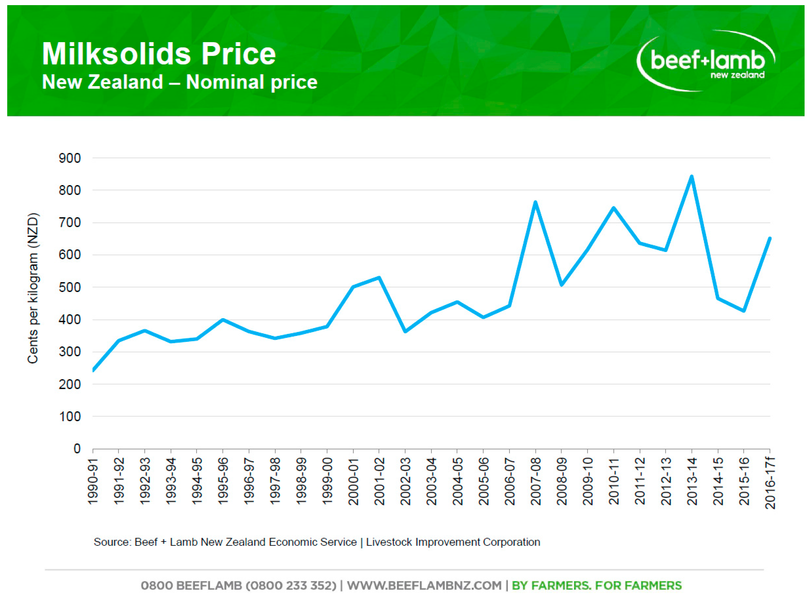
All commodity prices have fluctuated; however, mutton and lamb prices have moved together and all cattle beef prices are also highly correlated. Figure 1, Figure 2 and Figure 3 show the fluctuation in commodity prices which were used to fit “normal distributions” to farm income streams. Sheep meat prices and milk solids prices fluctuated more than beef prices. Sheep and dairy prices were fitted with a standard deviation of 20% and 13%, respectively, whilst beef prices were fitted with a standard deviation of 10%.
Climatic correlation was found as sheep meat prices peaked during 2011 which was a wet year throughout New Zealand with frequent summer rainfall. The coastal lower West North Island recorded 1297 mm of rain, which is considerably more than the 30-year average of 921 mm. This was followed in 2012 by a nationwide drought, where the LWNI recorded 778 mm of rainfall and little summer rainfall [3,4]. There was about a $100 difference in lamb prices between these years. In wet summers farmers can hold and finish their stock, as there is plenty of feed on the farm, so the farmers do not need to sell unless the price is high, whereas in drought years farmers must de-stock their properties or buy feed, which tends to be expensive in drought years, and are forced to sell stock on a buyers’ market. The correlation tool in “@Risk” software was used to add correlations for sheep and beef prices with rainfall, the price of hay was negatively correlated to rainfall, and as the dairy farm is irrigated no climate correlation was undertaken. These correlations impact the distributions in the risk profile. As sheep prices are much more variable in national droughts and wet summers than localised weather events, which are much more common, a weak correlation was used as an input for demonstration purposes. Cattle prices are much more stable than sheep prices so no correlation to rainfall was applied to cattle. A “normal distribution” was fitted to rainfall for the LWNI accounts with a mean of 921 mm and a standard deviation of 150 mm. Prices for individual sheep and cattle were estimated from sales data, wool sold as greasy from farm and hay bales as 20 kg bales yielding 15 kg dry matter [7,10], (Table 1). Other analysts may choose to fit alternative distributions and apply different standard deviations or correlations depending on their outlook of the farm system, as each simulation takes a few seconds many scenarios may be considered.
The data inputs that have the greatest effect on dairy farm financial performance had normal distributions fitted. Feed grazing and purchased feed are heavily correlated and were fitted with a 70% correlation (see Table 2). The price dairy farmers are willing to pay to have their animals grazed off farm is very dependent on the price of supplementary feed products [9].
The model accounts were then run in “@Risk” to produce Monte Carlo simulations using the defined functions at a setting of 5000 iterations for each farm type. At this number of iterations, with the values for maximum, minimum, mean, and standard deviation for outputs after each simulation, a stable result is achieved.
2.1. Sheep and Beef
The base accounts for the sheep and beef simulation are shown in Table 3. Note that the farm has decided not to rear replacement sheep which provides an opportunity to earn grazing income (dairy support) and provides cash by reducing the value of the livestock inventory. This is done so as to evaluate changes to the production system using risk profiling. Costs were estimated from an economic survey of class 3 farm (hard hill country) production and weighted by hectares farmed [8]. The farm accounts are set out as would be expected in generally accepted accounting practice in New Zealand.
2.2. Dairy
3. Results
3.1. Monte Carlo Simulation Reports
3.2. Results Summary
The results show that the sheep and beef model farm based on a large hard hill country station is not very profitable. The profit is heavily affected by the items in Figure 4b, the tornado chart. A tornado chart shows the impact individual inputs have on profit in descending order, for this simulation the price achieved for store lambs is the largest item with an impact on mean profit between negative $168,766 and positive $141,710. The farm had made a decision not to raise replacements, which provided a source of cash but may have affected profitability (Table 5). Hard hill country farms traditionally struggle to finish lambs to a standard required by the meat companies. Their lambs are mainly sold as store lambs when weaned for fattening by finishing farms. For this simulation only 15% of lambs weaned were sold as prime, the others were sold as store lambs.
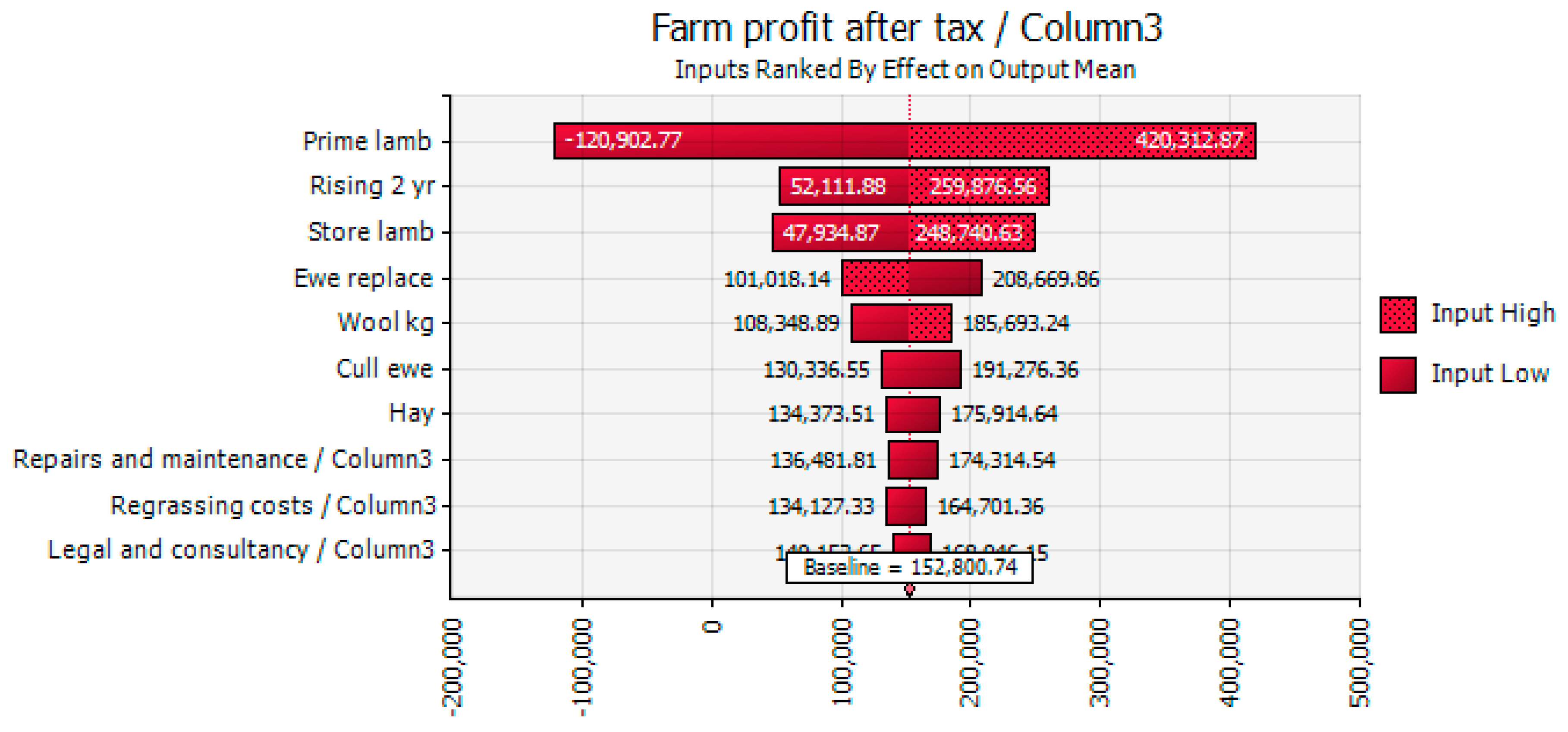
This example demonstrates the power of risk profiling and how it differs from standard variance analysis. The change contemplated with the parameters set leaves the farm with a baseline loss of $11,435 rather than a $7250 profit when 5000 Monte Carlo simulations are run. However, if by destocking the farm the percentage of prime lambs sold increases from 15% to 50% then the profitability changes. By improving the percentage of lambs finished the profitability changes to a baseline profit of $152,800 and the tornado graph shows the biggest impact on profitability is now prime lambs (see Figure 6). Although even in this scenario the standard deviation of after tax profit is $177,000, which is expected in New Zealand pastoral production systems [11].
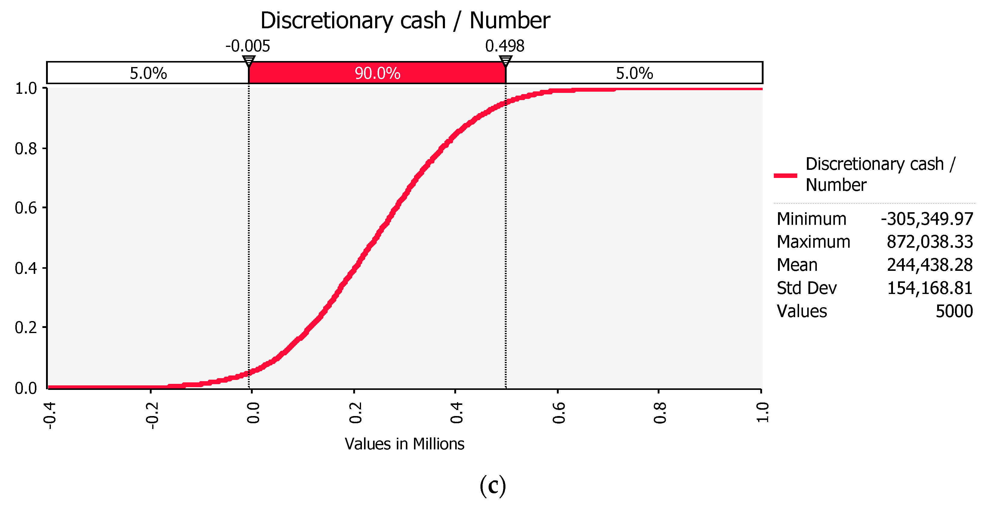
The model dairy farm produces a baseline profit of $244,500, slightly more than the base budget of $231,300 (Table 3), with a standard deviation of $226,400 (Figure 5a). The software is also able to goal seek a cell value, which can be useful for decision making. For the dairy farm, a breakeven price of $5.20 kg−1 milk solids using this farming system was derived.
4. Discussion
Provided some thought and research is undertaken by the consultant to provide useful functions to farm production inputs and outputs, risk profiling software can be a great tool in providing quick management feedback regarding the risk factors of a decision or of a farm in general [12,13].
The two pastoral farms considered in this study are quite different, although the software is useful in both situations. The highly leveraged dairy farm which is only 5% of the land area of the hill country station has a much higher baseline profit. This baseline profit is only slightly higher than the standard deviation of the profit, which reflects the sharp movements in the commodity price of milk solids, which means that for around 17% of the time the dairy farm may operate at a loss [2].
One of the ways of mitigating milk solids price variability risk in a dairy situation is to employ a low input strategy. In the dairy farm modelled in Table 4, the farm purchases around $390,000 of supplementary feed (around 1300 tonnes), which converts to around half the milk solids produced. To enable feeding out, some infrastructure components such as feed pads, wintering barns, and feed conveying machinery is often required. In addition, higher stocking rates increase animal health costs and frequently more regressing is required to offset the damage done to pastures. A low input strategy would reduce the costs, lowering the breakeven point to less than $5.20 kg−1 milk solids, but would reduce the profit when milk solid prices were above the breakeven point.
The low input option in this example would half the number of cows farmed and reduce the income by approximately $950,000. It would also reduce farm working expenses by around $600,000 and would negate the capital costs of providing feeding structures and infrastructure, which would reduce interest expense and principal payments. Other cost reductions would be in effluent reticulation, repairs and maintenance, and labour.
Risk profiling may be an important tool for New Zealand farmers as they prepare for the impacts of climate change and environmental constraints. Some climate modelling predicts more severe rain events and a drier east coast climate with more severe droughts [3]. The costs of flood damage are likely to increase and even farms which do not normally flood will be likely to be more prone to gully erosion, slips, and slumps. The costs of drains, fencing, and tree planting may offset some of the costs of these events and are suitable for modelling.
Distributions that reflect these risks and costs and benefits of changes in farm management are ideal for future proofing a farm. For example, deep rooting drought tolerant pasture crops such as plantain Plantigo lanceolate, chicory Circhorium intybus, and lucerne (alfalfa) Medicago sativa are growing in popularity on properties suffering more frequent autumn droughts. These crops enable farmers to finish stock and achieve prime rather than store prices, therefore, enabling them to avoid being forced on a buyers’ market. The alternative to providing fodder crops is to finish stock earlier. Early lambing enables prime lambs to be finished before feed is in short supply. However, it also means young lambs are born in cold wet conditions which can lead to high mortality [14]. Winter lambing also means that ewes are feeding at a time that pasture is not growing vigorously and inevitably at a rate less than stock demand [15]. Farmers may mitigate the low pasture growth periods by feeding out or, when weather permits, by the addition of regular low application rates of nitrogenous fertilizers and gibberellic acid. It may be economic in some situations to lamb indoors, a common practice in Europe but not undertaken in New Zealand.
5. Conclusions
Farmers as risk managers are looking to mitigate the risks of climate to optimize a production system that is heavily climate dependent. Climatic variation has an impact on costs and can affect commodity prices, which are also subject to variation through market forces. Providing a means of evaluating production systems to understand the risk profile with a view to mitigating these risks is an important tool.
Risk profiling is a far more powerful tool than variance analysis, which is the common means of assessing farm risk. A farm advisor may examine a budget using variance analysis and vary a few items such as meat and dairy prices, or costs such as supplementary feed. However, this does not look at the whole picture and the production base in a natural environment. As long-term weather forecasting has improved, the impact of climate on farm production can be inputted to a risk profile and better farm decisions can be made. Predictions of a mild wet spring may correlate to more prime lambs being finished, more hay and baleage being made, a need to protect flat paddocks from stock to prevent pugging, higher regressing costs, and more likelihood of farm surplus. Similarly, if a series of tropical depressions is predicted, the likelihood of flood damage and associated large increases in repairs and maintenance can be profiled with a much greater chance of a farm deficit. Farming is, therefore, very well suited to risk profiling, which will likely add value to management information systems as the effects of climate change impacts.
Acknowledgments
Funds to publish this paper were provided by MDPI author vouchers and by the Institute of Agriculture and the Environment, Massey University, Palmerston North 4410, new Zealand.
Author Contributions
Miles Grafton conceived the commentary; Miles Grafton and Michael Manning planned the commentary; Miles Grafton undertook the research and analysis; Michael Manning planned the discussion and conceived the analysis of changes to production systems.
Conflicts of Interest
The authors declare no conflict of interest.
References
- Jose, H.D.; Valluru, R.S.K. Insights from the Crop Insurance Reform Act of 1994. Agribusiness 1997, 13, 587–598. [Google Scholar] [CrossRef]
- Shadbolt, N.M.; Olubade-Awasole, F.; Gray, D.; Dooley, E. Risk—An Opportunity or Threat for Entrepreneurial Farmers in the Glbal Food Market? Int. Food Agribus. Manag. Rev. 2010, 13, 75–97. [Google Scholar]
- Fauchereau, N.; Chappell, P.; Griffiths, G.; Sturman, J.; Wilsman, A. State of the Climate. NIWA Science and Technology Survey No.57. 2013. Available online: www.niwa.co.nz (accessed on 4 November 2014).
- Grafton, M.C.E.; Yule, I.J. Farm system risk analysis: Building a farm risk profile to improve farm economic outcomes. In Moving Farm Systems to Improved Nutrient Attenuation; Currie, L.D., Burkitt, L.L., Eds.; Occassional Report No. 28; Fertilizer and Lime Research Centre, Massey University: Palmerston North, New Zealand, 2015; 12p, ISSN 0112–9902. Available online: http://flrc.massey.ac.nz/publications.html (accessed on 1 August 2017).
- Grafton, M.C.E. Chinese Stockpiling Curdles New Zealand’s Milk, Policy Forum. 2016. Available online: https://www.policyforum.net/chinese-stockpiling-curdles-new-zealands-milk/ (accessed on 8 February 2017).
- Dairy NZ Ltd., Livestock Improvement Corporation. New Zealand Dairy Statistics 2015–2016. Available online: https://www.dairynz.co.nz/publications/dairy-industry/new-zealand-dairy-statistics-2015–16/ (accessed on 19 April 2017).
- Beef and Lamb New Zealand, Economic Service Sheep and Beef Farm Survey. Available online: http://www.beeflambnz.com/information/on-farm-data-and-industry-production/benchmarking-data/ (accessed on 3 May 2017).
- Anon, Ohorea Station. 2014. Available online: http://www.atihau.com/ohorea.html (accessed on 31 July 2017).
- Journeaux, P. Canterbury Dairy Farm Monitoring Report. 2013. Available online: www.mpi.govt.nz (accessed on 1 November 2014).
- Anon, Facts and Figures Dairy NZ, 92 Pages, Page 19. 2012. Available online: https://www.dairynz.co.nz/publications/dairy-industry/facts-and-figures/ (accessed on 15 May 2017).
- Martin, S.; Shadbolt, N. Risk Management. In Farm Management in New Zealand; Shadbolt, N., Martin, S., Eds.; Oxford University Press: Victoria, Australia, 2005; Chapter 10; pp. 201–220. ISBN 978-0-19-558389-2. [Google Scholar]
- Martin, S.K. Risk perceptions and management responses to risk in pastoral farming in New Zealand. Proc. N. Z. Soc. Anim. Prod. 1994, 54, 363–368. Available online: http://nzsap.org/proceedings/browse (accessed on 19 September 2017).
- Hardaker, J.B.; Huirne, R.B.M.; Anderson, J.R.; Lien, G. Coping with Risk in Agriculture, 2nd ed.; CAB International: Wallingford, UK, 2004. [Google Scholar]
- Morris, C.A.; Hickey, S.M.; Clarke, J.N. Genetic and environmental factors affecting lamb survival at birth and through to weaning. N. Z. J. Agric. Res. 2002, 43, 518–524. [Google Scholar] [CrossRef]
- Monteath, M.A. Effect of submaintenance feeding of ewes during mid-pregnancy. Proc. N. Z. Soc. Anim. Prod. 1971, 31, 105–113. Available online: http://nzsap.org/proceedings/browse (accessed on 19 September 2017).
Figure 1.
A 10-year movement in lamb prices in New Zealand is shown [3].
Figure 1.
A 10-year movement in lamb prices in New Zealand is shown [3].
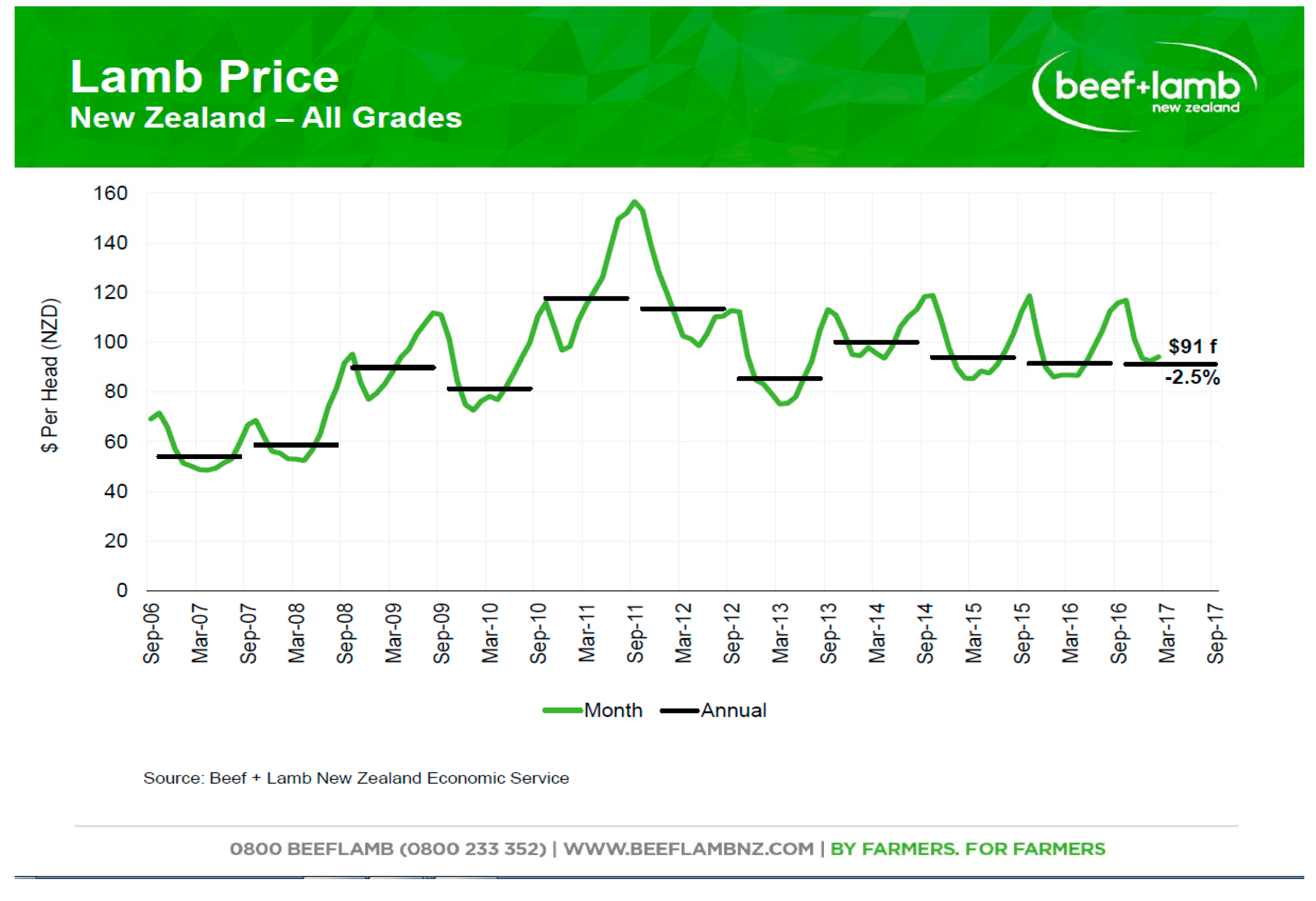
Figure 2.
A 10-year movement in milksolids prices in New Zealand is shown [3].
Figure 2.
A 10-year movement in milksolids prices in New Zealand is shown [3].

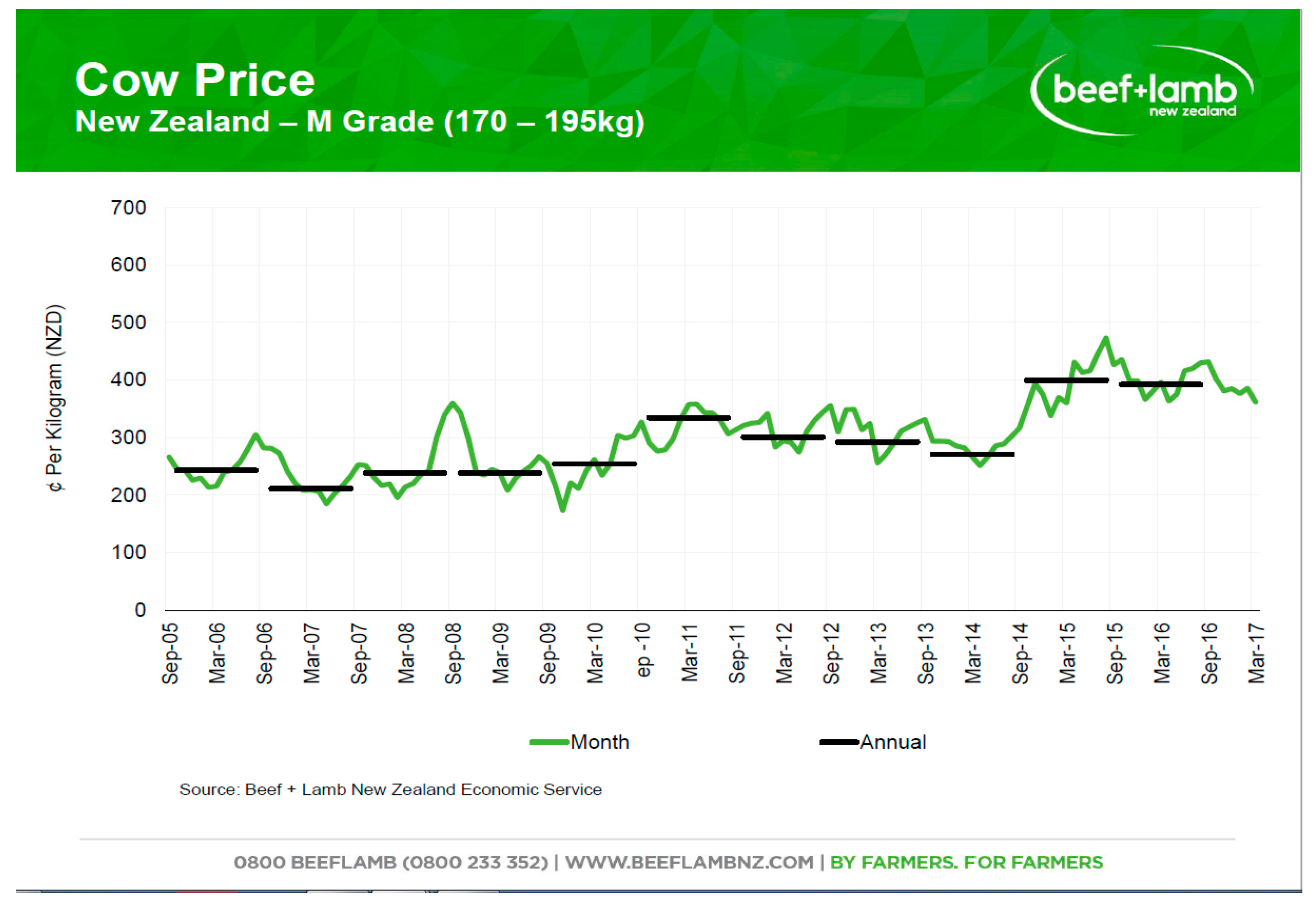
Figure 3.
A 10-year movement in cow meat prices in New Zealand is shown [3].
Figure 3.
A 10-year movement in cow meat prices in New Zealand is shown [3].

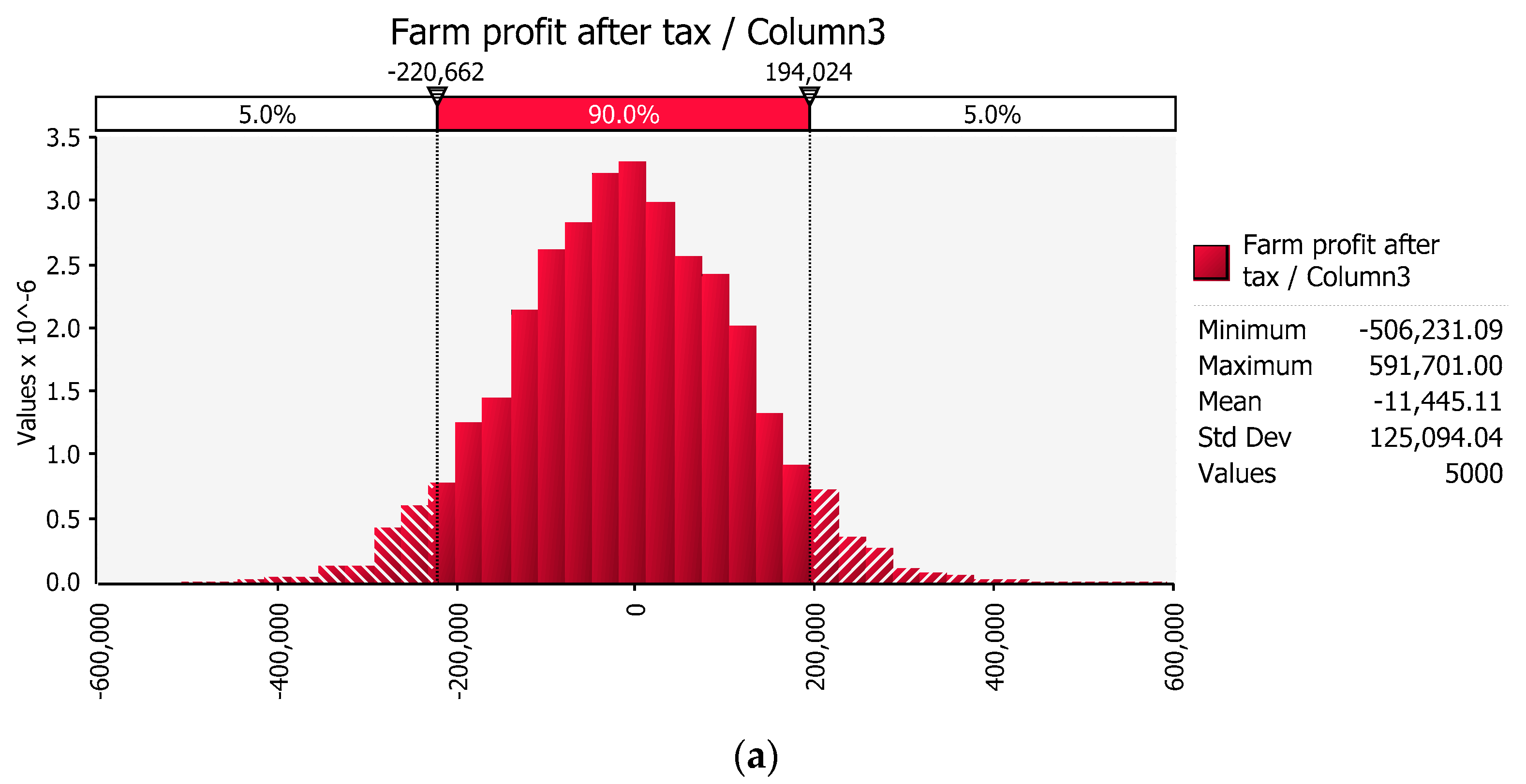
Figure 4.
“@Risk” simulated risk profile for the sheep and beef farm, showing distribution of after tax profit (a); tornado chart (b); cumulative distribution of profits (c).
Figure 4.
“@Risk” simulated risk profile for the sheep and beef farm, showing distribution of after tax profit (a); tornado chart (b); cumulative distribution of profits (c).


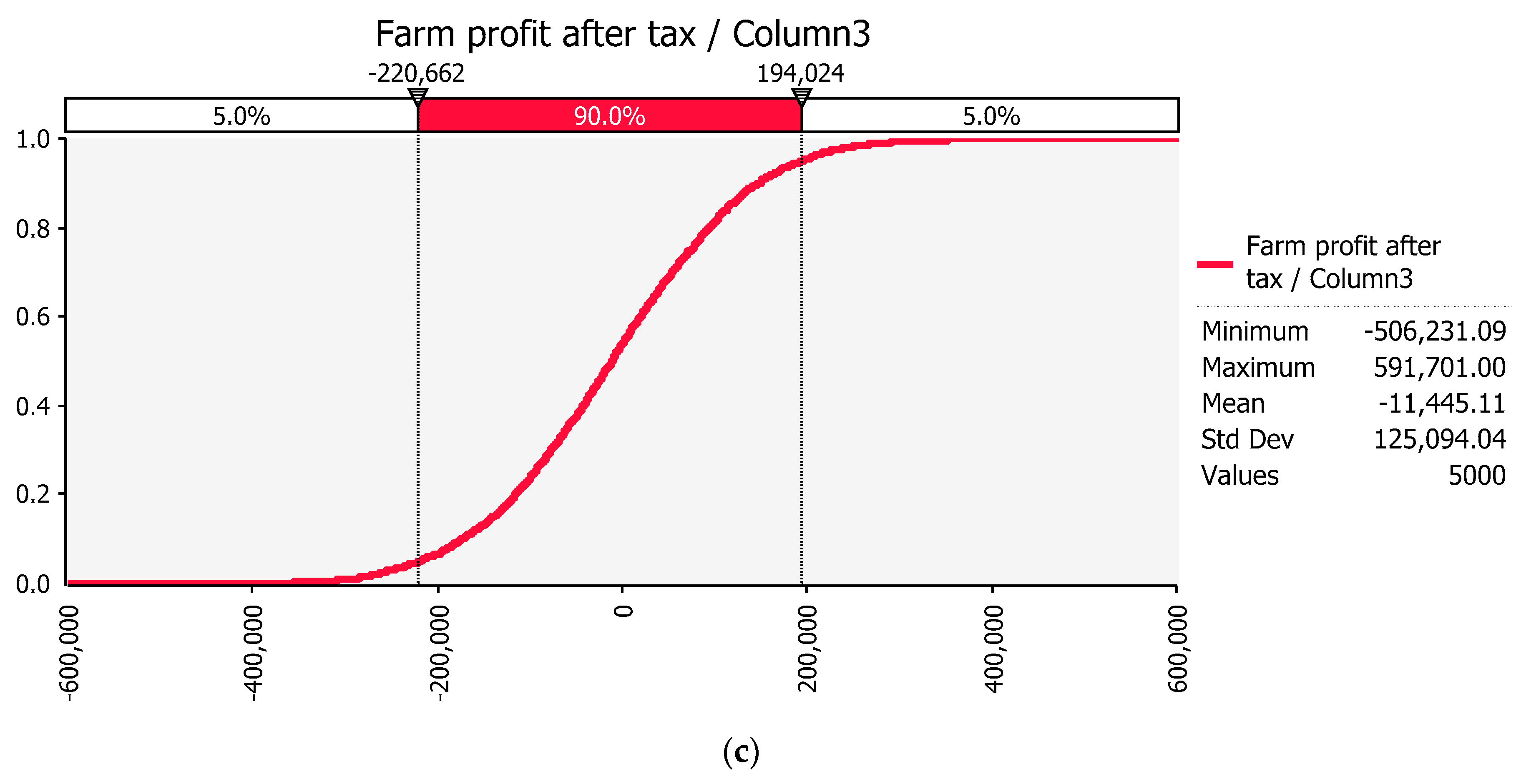
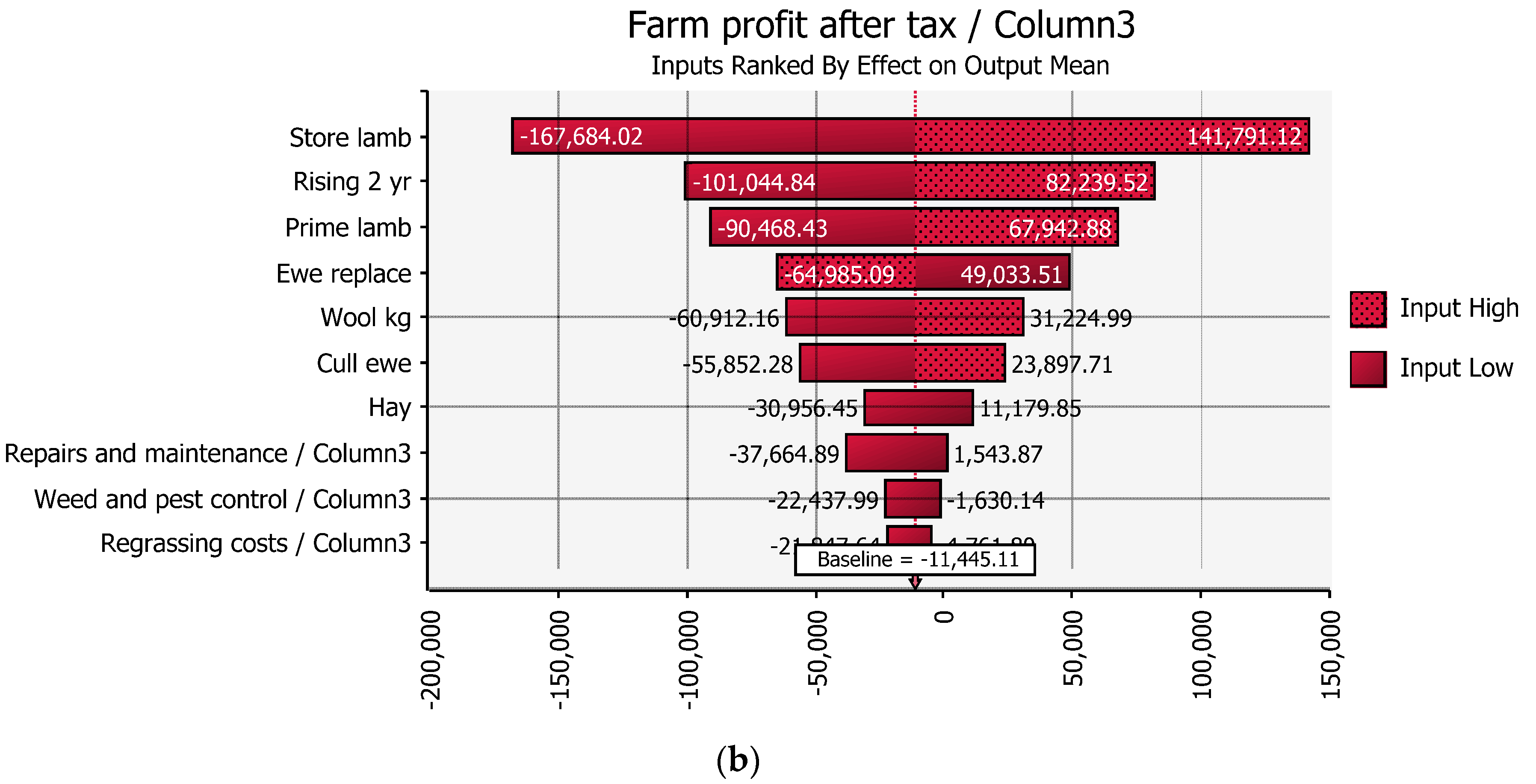
Figure 5.
“@Risk” simulated risk profile for the dairy farm, showing distribution of discretionary cash (a); tornado chart (b); and cumulative distribution of discretionary cash (c).
Figure 5.
“@Risk” simulated risk profile for the dairy farm, showing distribution of discretionary cash (a); tornado chart (b); and cumulative distribution of discretionary cash (c).


Figure 6.
Simulated risk profile with 5000 iterations when 50% rather than 15% of lambs are sold as prime.
Figure 6.
Simulated risk profile with 5000 iterations when 50% rather than 15% of lambs are sold as prime.

Table 1.
Modelling price inputs, correlation to rainfall, and 5–95% confidence levels for a sheep station in lower Western North island of New Zealand (LWNI) using a normal distribution.
Table 1.
Modelling price inputs, correlation to rainfall, and 5–95% confidence levels for a sheep station in lower Western North island of New Zealand (LWNI) using a normal distribution.
| Stock Type | Median Price | Correlate Rain | Std. Dev. % | 5% Conf. | 95% Conf. |
|---|---|---|---|---|---|
| Store lamb | 63.00 | 0.48 | 10 | 52.64 | 73.36 |
| Prime lamb | 91.00 | 0.48 | 20 | 61.00 | 120.90 |
| Replace ewe | 88.28 | 0.48 | 10 | 73.80 | 102.80 |
| Cull ewe | 60.00 | 0.48 | 10 | 50.13 | 69.87 |
| Weaner | 140.00 | 10 | 117.00 | 163.00 | |
| Rising 1 year | 450.00 | 10 | 376.00 | 524.00 | |
| Rising 2 year | 890.00 | 10 | 744.00 | 1036.00 | |
| Wool $ kg−1 | 2.80 | 10 | 2.34 | 3.26 | |
| Hay bales $ | 7.50 | −0.56 | 10 | 6.27 | 8.73 |
| Rainfall mm | 921 | 1.00 | 16 | 674 | 1168 |
Table 2.
Modelling price inputs, correlation to rainfall, and 5–95% confidence levels for a Canterbury dairy farm.
Table 2.
Modelling price inputs, correlation to rainfall, and 5–95% confidence levels for a Canterbury dairy farm.
| Stock Type | Median Data | Std. Dev. % | 5% Conf. | 95% Conf. |
|---|---|---|---|---|
| Cows milked | 709 | 5 | 688 | 742 |
| Cows wintered | 763 | 5 | 740 | 800 |
| Feed grazing ($) | 240,803 | 10 | 201,166 | 280,363 |
| Feed other ($) | 149,440 | 10 | 124,855 | 174,007 |
| Milk solids per cow | 410 | 10 | 376 | 444 |
| Milk solids $ kg−1 | 6.00 | 13 | 4.68 | 7.32 |
| Cull cows ($) | 504 | 10 | 310 | 724 |
| Milking cows ($) | 1000 | 10 | 835 | 1164 |
| Weaner heifers ($) | 140 | 10 | 117 | 163 |
| Re-grassing ($) | 13,370 | 10 | 12,373 | 15,532 |
Table 3.
The base set of accounts used for the sheep and beef Monte Carlo simulation.
| Item | Amount | Cost ($) | Revenue ($) |
|---|---|---|---|
| Ewes to lamb | 19,400 | ||
| Cattle 1 year rising | 1074 | ||
| Lambing (%) | 120 | ||
| Lamb sales | 23,280 | 1,564,416 | |
| Sheep sales | 4730 | 283,800 | |
| Sheep replacements | 4800 | 423,744 | |
| Cattle sales | 899 | 800,110 | |
| Cattle (weaners) | 330 | 46,200 | |
| Wool (kg) | 116,600 | 326,480 | |
| Grazing income as hay bales | 25,000 | 187,500 | |
| Net cash income | 2,692,362 | ||
| Farm working expenses | |||
| Permanent/casual wages | 296,400 | ||
| ACC (accident insurance) | 13,931 | ||
| Total labour expenses | 310,331 | ||
| Animal health/breeding | 113,730 | ||
| Electricity | 64,950 | ||
| Feed (feed crops and other) | 54,710 | ||
| Fertilizer and Lime | 537,000 | ||
| Re-grassing, weed, and pest | 78,929 | ||
| Freight | 74,640 | ||
| Shearing expenses | 116,720 | ||
| Vehicle running and fuel | 209,766 | ||
| Repairs and maintenance | 173,888 | ||
| Total other working | 1,424,333 | ||
| Communication/administration | 41,034 | ||
| Accountancy and legal | 16,276 | ||
| Local government charges | 54,904 | ||
| Insurances | 49,744 | ||
| Total Overhead | 161,958 | ||
| Total farm working expenses | 1,896,622 | ||
| Interest | 110,613 | ||
| Stock inventory adjustment | (394,950) | ||
| Depreciation | 280,092 | ||
| Farm profit before tax | 10,085 | ||
| Tax | (2824) | ||
| Profit after tax | 7261 | ||
| Allocation funds | |||
| Add back depreciation | 280,092 | ||
| Reverse stock adjustment | 394,950 | ||
| Principal payments | (45,595) | ||
| Drawings | (158,512) | ||
| Capital purchases | (131,940) | ||
| Cash surplus | 346,256 |
Table 4.
The base set of accounts used for the dairy farm Monte Carlo simulation.
| Item | Amount | Cost ($) | Revenue ($) |
|---|---|---|---|
| Effective area (ha) | 210 | ||
| Milk solids per cow milked | 410 | ||
| Milk solids per hectare | 1396 | ||
| Total milk solids | 293,150 | ||
| Milk solids advance to 30 June ($/kg) | 4.92 | ||
| Milk solids deferred ($/kg) | 1.08 | ||
| Cows wintered | 769 | ||
| Cull cows | 180 | 90,720 | |
| Replacement heifers | 180 | 25,200 | |
| Cows milked peak | 715 | ||
| Net cash income | 1,824,420 | ||
| Farm working expenses | |||
| Total labour expenses | 243,122 | ||
| Animal health/breeding | 102,960 | ||
| Dairy shed/electricity | 85,085 | ||
| Feed (feed crops and other) | 392,100 | ||
| Fertilizer Ag-lime freight | 154,440 | ||
| Re-grassing, weed, and pest | 18,590 | ||
| Vehicle, fuel, and Repairs & Maintenance | 144,430 | ||
| Total other working | 897,605 | ||
| Communication and sundry | 15,558 | ||
| Accountancy legal administration | 11,440 | ||
| Water local government | 39,325 | ||
| Insurances | 25,039 | ||
| Total overhead | 91,362 | ||
| Total farm working expenses | 1,232,089 | ||
| Interest | 330,000 | ||
| Dividend dairy company wet share | 94,421 | ||
| Stock value adjustment | - | ||
| Depreciation | 35,780 | ||
| Farm profit before tax | 320,972 | ||
| Tax | (89,872) | ||
| Profit after tax | 231,100 | ||
| Allocation funds | |||
| Add back depreciation | 35,780 | ||
| Reverse stock adjustment | - | ||
| Principal payments | (140,000) | ||
| Drawings | (85,000) | ||
| Cash surplus | 41,880 |
Table 5.
Change in inventory by stock class to provide $394,950 cash.
| Stock | Open | $/head | Open $ | Close | $/head | Close $ |
|---|---|---|---|---|---|---|
| Ewes | 14,600 | 60 | 876,000 | 19,400 | 60 | 1,164,000 |
| Hoggets | 4800 | 88 | 422,400 | |||
| Cattle 1 year | 899 | 450 | 404,550 | 320 | 450 | 144,000 |
| Cattle 2 year | 899 | 890 | 800,110 | 899 | 890 | 800,110 |
| Cows | 1100 | 890 | 979,000 | 1100 | 890 | 979,000 |
| Total | 22,298 | 3,482,060 | 21,719 | 3,087,110 |
© 2017 by the authors. Licensee MDPI, Basel, Switzerland. This article is an open access article distributed under the terms and conditions of the Creative Commons Attribution (CC BY) license (http://creativecommons.org/licenses/by/4.0/).
Share and Cite
MDPI and ACS Style
Grafton, M.; Manning, M. Establishing a Risk Profile for New Zealand Pastoral Farms. Agriculture 2017, 7, 81. https://doi.org/10.3390/agriculture7100081
AMA Style
Grafton M, Manning M. Establishing a Risk Profile for New Zealand Pastoral Farms. Agriculture. 2017; 7(10):81. https://doi.org/10.3390/agriculture7100081
Chicago/Turabian StyleGrafton, Miles, and Michael Manning. 2017. "Establishing a Risk Profile for New Zealand Pastoral Farms" Agriculture 7, no. 10: 81. https://doi.org/10.3390/agriculture7100081
Note that from the first issue of 2016, this journal uses article numbers instead of page numbers. See further details here.