Article

Practical Applications of a Multisensor UAV Platform Based on Multispectral, Thermal and RGB High Resolution Images in Precision Viticulture

by
Alessandro Matese
* and
Salvatore Filippo Di Gennaro
Institute of Biometeorology (IBIMET), National Research Council (CNR), Via Caproni 8, 50145 Florence, Italy
*
Author to whom correspondence should be addressed.
Agriculture 2018, 8(7), 116; https://doi.org/10.3390/agriculture8070116
Submission received: 30 May 2018 / Revised: 19 July 2018 / Accepted: 20 July 2018 / Published: 23 July 2018
(This article belongs to the Special Issue Precision Agriculture)

Abstract

:
High spatial ground resolution and highly flexible and timely control due to reduced planning time are the strengths of unmanned aerial vehicle (UAV) platforms for remote sensing applications. These characteristics make them ideal especially in the medium–small agricultural systems typical of many Italian viticulture areas of excellence. UAV can be equipped with a wide range of sensors useful for several applications. Numerous assessments have been made using several imaging sensors with different flight times. This paper describes the implementation of a multisensor UAV system capable of flying with three sensors simultaneously to perform different monitoring options. The intra-vineyard variability was assessed in terms of characterization of the state of vines vigor using a multispectral camera, leaf temperature with a thermal camera and an innovative approach of missing plants analysis with a high spatial resolution RGB camera. The normalized difference vegetation index (NDVI) values detected in different vigor blocks were compared with shoot weights, obtaining a good regression (R2 = 0.69). The crop water stress index (CWSI) map, produced after canopy pure pixel filtering, highlighted the homogeneous water stress areas. The performance index developed from RGB images shows that the method identified 80% of total missing plants. The applicability of a UAV platform to use RGB, multispectral and thermal sensors was tested for specific purposes in precision viticulture and was demonstrated to be a valuable tool for fast multipurpose monitoring in a vineyard.

1. Introduction

In modern viticulture, the concept of precision viticulture has been well defined [1], namely the application of a series of methods and technologies developed to meet the need to maximize the oenological potential of the territory and optimize agronomic inputs in the vineyard in order to minimize costs and protect environmental sustainability. This is a differentiated approach according to the real needs of each vineyard or sections of it. The introduction of new technologies to support vineyard management can therefore improve efficiency and product quality while reducing the environmental impact of the treatments necessary to safeguard the state of health of the plants. Recent technological developments have led to tools that can provide the winemaker with the means to monitor and control many aspects of the vine growing environment. In the last decade, there has been a progressive diffusion of new monitoring instruments, i.e., remotely piloted aircraft known as UAVs (unmanned aerial vehicles), or more commonly, drones [2,3,4]. The advantage of these platforms for remote sensing applications is the high spatial resolution on the ground, centimeter, and the possibility of a highly flexible and timely control, due to reduced planning time. These characteristics make them ideal especially in the medium–small agricultural systems that are typical of many Italian viticulture areas of excellence. UAV can be equipped with a wide range of sensors useful for several applications.
Multispectral remote sensing images give an accurate description of variability within a vineyard through the canopy response to light absorption and reflection phenomena. Among several vegetation indices derived from remotely sensed images, the normalized difference vegetation index (NDVI) [5] has a strong relationship with biomass and photosynthetic activity [6,7,8,9,10]. Furthermore, NDVI has been found to correlate well with grape quality properties, such as phenolic substances and anthocyanins at harvest [11], but not always [12,13]. In recent years, the adoption of UAV platforms for remote sensing has overcome some of the limits of satellite-based and aircraft based observations, in terms of flexibility of data acquisition, scheduling and high ground resolution [14,15,16].
High resolution thermal images acquired by UAV allow a detailed characterization of canopy top temperature in a vineyard [17] and could be a useful tool for water stress detection. It is well known that even short-term water deficits affect growth processes and induce stomatal closure, which reduces transpiration and, consequently, evaporative cooling, resulting in an increase in leaf temperature. Studies on this temperature increase and its correlation with crop water stress have been conducted using thermal infrared thermometers over a period of decades. Jones [18] suggested that greater precision in irrigation management could potentially be obtained using plant-based responses rather than soil water status measurements. However, this monitoring is time-consuming. The crop water stress index (CWSI), a thermal-derived indicator of water deficit based on canopy temperature measurements has been used to assess the water status of crops such as grapevine [19], French beans [20], wheat [21], rice [22], maize [23] and cotton [24].
RGB imagery became a useful tool for different kinds of applications due to its very high resolution. A common problem in trellising systems is the occurrence of missing plants (also referred to as voids) on the vine rows. This is usually due to the premature death of a vine, and apart from a consequent lowering of vineyard production, it poses problems from a remote sensing point of view. Indeed, not only can it be an obstacle to vine row recognition and thus to automatic processing of the aerial map [25] but it can also induce errors in the estimation of vigor zones inside vineyards and affect the results of the application of precision agriculture techniques. The aim of this study is to illustrate some results that can be obtained by monitoring the spectral response of the crops at low altitude with very high-resolution sensors. Specifically, the paper describes the use of a single UAV platform with three different imaging sensors for three common applications in precision viticulture: missing plant detection using an RGB camera, vegetative vigor monitoring using a multispectral camera and water stress detection using a thermal camera.

2. Materials and Methods

2.1. Experimental Sites

The research was conducted in three experimental sites located in areas of excellence of Tuscan viticulture (Italy): Chianti Classico (sites A and B) and Montalcino (site C) (Figure 1). Vineyard details are described in Table 1.

2.2. Remote Sensing Measurements

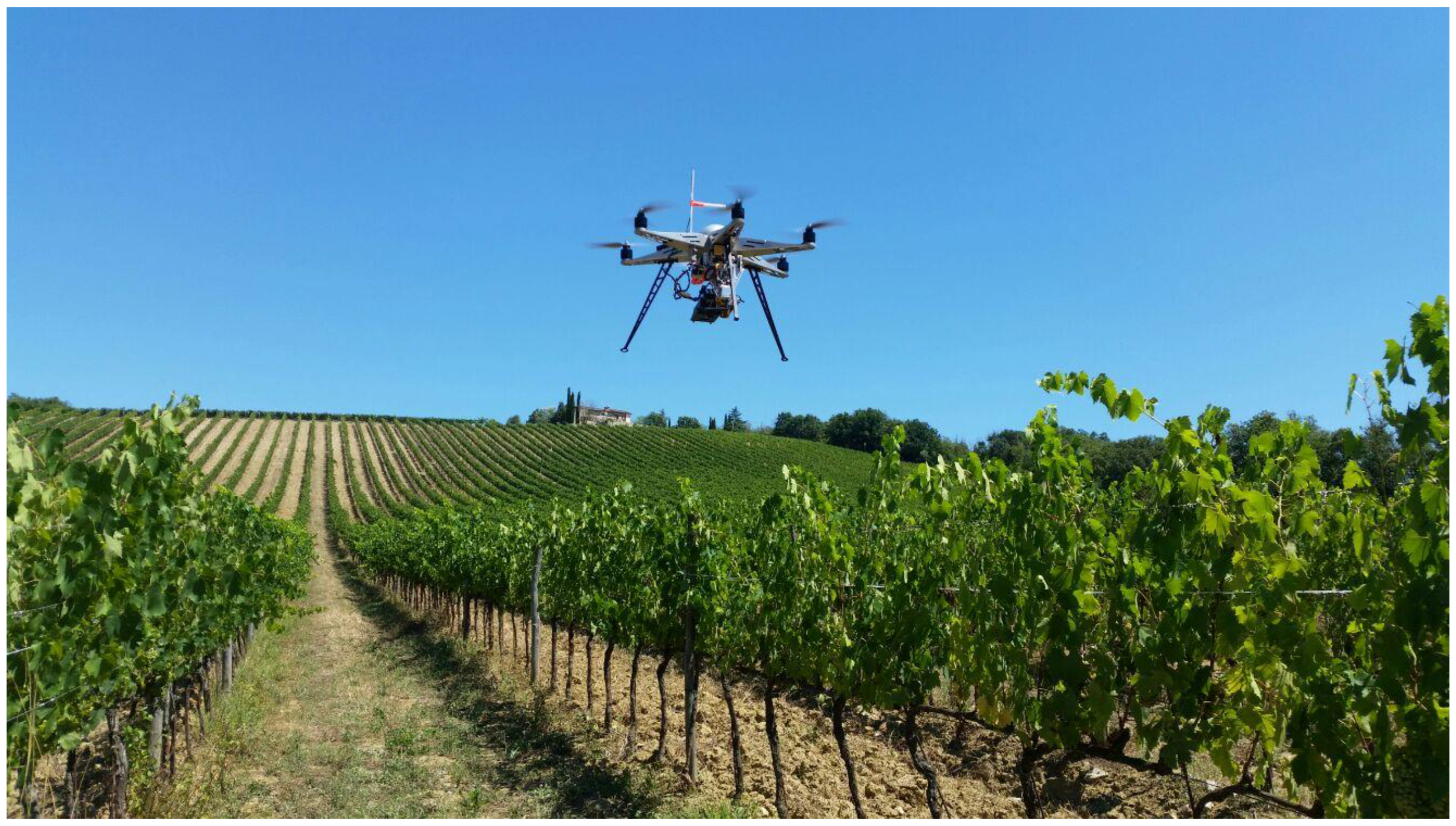
2.2.1. UAV Platform and Payload

Flight campaigns were performed using an open-source UAV platform (Figure 2) consisting of a modified multi-rotor Mikrokopter (HiSystems GmbH, Moomerland, Germany).
Autonomous flight is managed by an on-board navigation system, which consists of a GPS module (U-blox LEA-6S, U-blox AG, Thalwil, Switzerland) connected to a navigation board (Navy-Ctrl 2.0, HiSystems GmbH, Moomerland, Germany) and a flight control unit (Mikrokopter Flight Controller ME V2.1, HiSystems GmbH, Moomerland, Germany) controlling six brushless motors. Two communication systems consisting of a duplex transmitter at 2.4 GHz (Graupner, Kirchheim, Germany) and a WiFi module (Mikrokopter, HiSystems GmbH, Moomerland, Germany) at 2.4 GHz allow control of the UAV navigation and monitoring of flight parameters, while a WiFi module provides video data transmission at 5.8 GHz ensuring real-time image acquisition control by the ground operator. The flight planning was managed through Mikrokopter Tool software (V2.20, HiSystems GmbH, Moomerland, Germany), which allows a route of waypoints to be generated as a function of the sensor Field of View (FOV) required overlap between images and ground resolution. Maximum payload is approximately 1 kg, ensuring 15 min of operating time with one 4S battery @11,000 mAh. A universal camera mount equipped with three servomotors allows accurate image acquisition through compensation of tilt and rolling effects.
The UAV was equipped with a Canon Eos M 18Mpx RGB camera (Canon Inc., Tokyo, Japan), a Tetracam ADC Snap multispectral camera (Tetracam, Inc., Gainesville, FL, USA) and a thermal camera (FLIR TAU II 320, FLIR Systems Inc., Wilsonville, OR, USA). Table 2 reports UAV camera specifications.

2.2.2. Flight Survey

The UAV flight campaigns were conducted in the experimental vineyards by a single flight at 70 m above ground level at midday, yielding a ground resolution of 0.01 m/pixel, 0.04 m/pixel and 0.09 m/pixel in RGB, multispectral and thermal images, respectively.
The multispectral and RGB cameras were set at 0.2 s triggering time, the first with fixed exposure and the second with automatic exposure. Thermal camera setting was chosen to acquire and store 20 images per second with fixed time exposure.
The waypoint route was generated to obtain more than 80% overlap among both photos (forward overlap) and flight lines (lateral overlap), in order to achieve the highest accuracy in the mosaicking elaboration step. The images were recorded in clear sky conditions.

3. UAV Image Processing

3.1. Multispectral Data Processing

Multispectral images acquired by UAV were mosaicked using Agisoft Photoscan Professional Edition 1.1.6 (Agisoft LLC, St. Petersburg, Russia). A polygon mesh was computed from the dense 3D point cloud and the pixel values of each image were then projected onto the mesh to create an orthomosaic. When combined with GPS positions, this process allows the creation of a high-resolution orthophoto and a digital elevation model (DEM) of the experimental site. Spectral calibration is needed to determine the center wavelength, spectral bandwidth and spectral response function of all spectral channels for the camera, and then monitor the spectrum stability and calibrate the wavelength shift based on the standard spectrum signal. Since the center wavelength and full width at half maximum (FWHM) were provided by the manufacturer, spectral calibration was not performed.
A vicarious calibration based on the absolute radiance method was chosen, given that digital number (DN) value for each pixel has a direct relationship (linear model) with the radiance detected by the sensor [26]. For this radiometric calibration process, images from three OptoPolymer (OptoPolymer, Werner Sanftenberg, Munich, Germany) homogeneous and Lambertian surface panels, with 95%, 50% and 5% reflectance, were acquired for each flight.
The filtering procedure of the pure vine canopy pixels was assessed with a digital elevation model (DEM) output produced from Agisoft Photoscan software (version 1.2.4, Agisoft LLC, St. Petersburg, Russia). The basis of the procedure was that rows have a greater height than the ground and can easily be discriminated by the Otsu global thresholding, an algorithm that allows discrimination of two different zones, in this case rows and ground [17].
The multispectral images obtained by UAV allowed the spatial variability in the vineyard to be evaluated in terms of vigor. The NDVI was computed according to the following equation:
NDVI = (NIR − RED)/(NIR + RED)
where NIR and RED are the spectral reflectance in near infrared and red bands, respectively [5].
The NDVI vegetation index was calculated for each pixel of the orthomosaic, and then two NDVI maps were elaborated using only pure canopy pixels (row filtering) and both canopy and ground pixels (without row filtering). The two maps were then interpolated to perform a classification in 5 classes (quintiles) of the entire vineyard. Following the vigor variability, six representative blocks within homogeneous areas were identified: three blocks in the high vigor zone (south) and three in the low vigor zone (north). A total of 25 sample vines for each block were harvested to determine pruning mass in the dormant period following the experimental season, and the total shoot fresh mass per vine was extrapolated. The NDVI values for the vines measured for pruning weight were determined using the average value of the blocks.

3.2. Thermal Data Processing

Brightness temperature measured by the thermal camera was converted to radiometric temperature assuming a leaf emissivity coefficient of 0.98 as reported by Jones and Vaughan [27]. Leaf radiometric temperature acquired in the thermal infrared spectral region allows maps of leaf temperature and then plant water deficit to be computed through the estimation of CWSI. CWSI was calculated using the equation [28,29]:
CWSI = (Tleaf − Twet)/(Tdry − Twet)
where Tdry and Twet represent the temperature of a stressed and non-stressed leaf condition, respectively, while Tleaf indicates the actual leaf surface radiometric temperature. Tleaf data in absolute temperature (K) were calculated from the thermal camera digital number (DN) using the empirical line method as reported by [9]. Radiometric calibration was done using three different colored panels (1 m × 1 m) at known temperature as reference.
Measurements were taken continuously every 10 s during the flight with a hand-held thermal camera (Flir i7, FLIR Systems Inc., Wilsonville, OR, USA). The procedure for estimating reference temperatures (Tdry and Twet) is crucial to obtain accurate water stress maps. The adopted methodology was proposed by Jones et al. [29]. Leaves of two vines were coated with Vaseline on both sides to prevent transpiration and stop cooling, simulating the leaf physiological response to water stress conditions. The wet reference was obtained by wetting both sides of the leaves of other two vines. Tdry and Twet were measured 30 min after applying Vaseline and 20 s after wetting, respectively. CWSI maps were obtained by an interpolation using a 50 m × 50 m window moving average of CWSI values for the pure canopy pixels (Figure 3b). A 50m size window was chosen due to the size of the vineyard for a better interpolation. Figure 3c shows the NDVI vigor map classified using percentiles, monitored the day before thermal acquisition. Following the vineyard vigor variability, three representative blocks were identified within homogeneous areas: one block in the high vigor zone (north), one in the medium (central) and one in the low vigor zone (south). Stomatal conductance was measured between 10 a.m. and 12 p.m. on two fully-expanded leaves per plant at the same physiological stage (from the eighth to the tenth leaf from the bottom) on five plants per block using the LI-6400XT portable photosynthesis system (LI-COR, Lincoln, NE, USA).

3.3. RGB Data Processing

Missing plant detection was performed starting from a georeferenced RGB orthomosaic of a plot (40 × 60 m) in an experimental vineyard with 0.01 m/pixel image spatial resolution.
The filtering procedure of the pure vine canopy pixels was assessed with a digital elevation model (DEM) output generated from RGB images and using Agisoft Photoscan software.
The vineyard was chosen to evaluate the methodological approach under extreme conditions, with different plant ages and spacing due to the fact that the vineyard was planted in 1973 and new vines have been added over time to replace dead plants, frequently with different spacing along the rows. A ground survey of missing plants was conducted at the end of the season in December 2017. Polygons were drawn from the filtered RGB mosaic with a size of 1.00 × 0.60 m similar to a single plant size. Specifically, the approach used to perform the classification of polygons in probability classes of plant presence was based on the count of pure canopy pixels present within each polygon. The zonal statistical output of the remote data extracted for each plant was then classified on a five-class scale from green to red, where green indicates a 100% certain plant presence and red indicates a 100% certain missing plant. A frequency distribution of pixel values was divided into five classes (quintiles), corresponding to 1/5 of the detected cases. The first quintile was chosen as class F1 (certain missing plant) representing 20% of the value distribution with less pixels, the fifth quintile as class F5 (high probability missing plant) that represents the last 20% of values with higher count of canopy pixels.

4. Results and Discussion

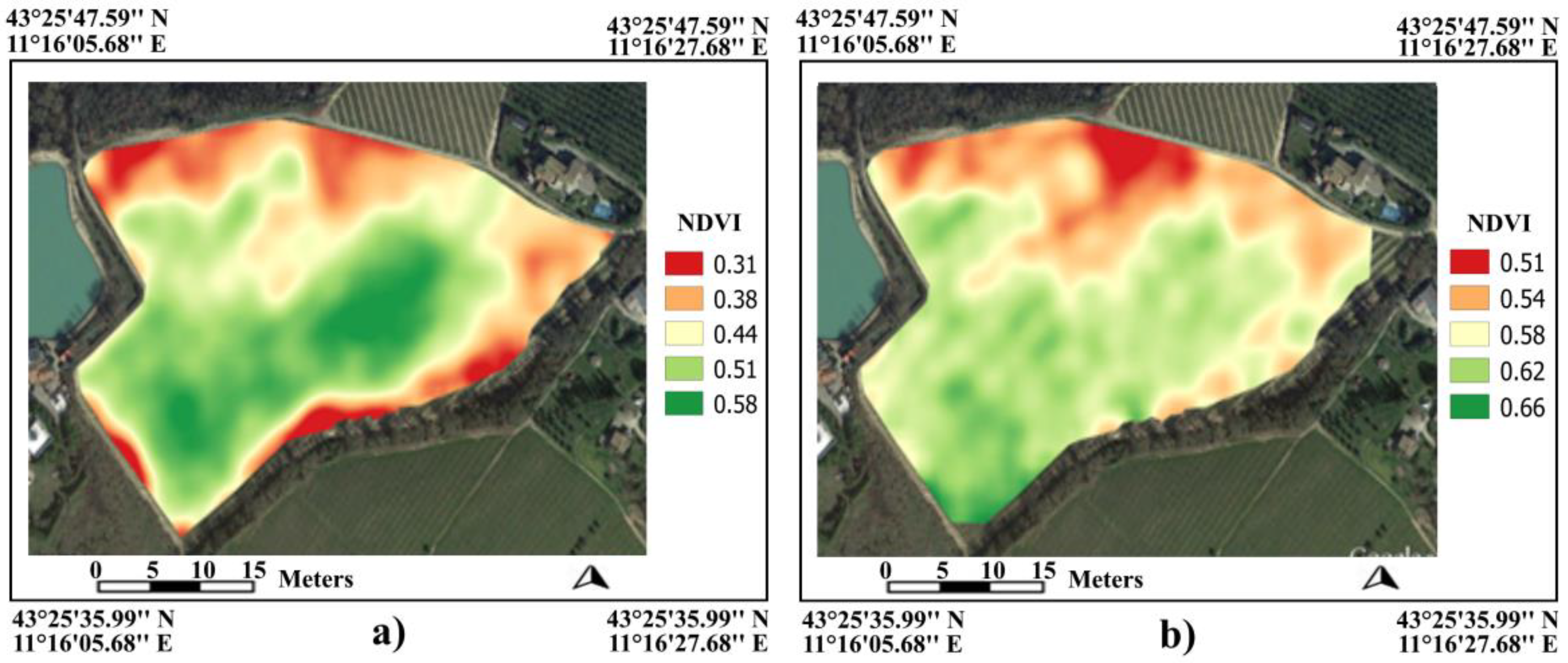
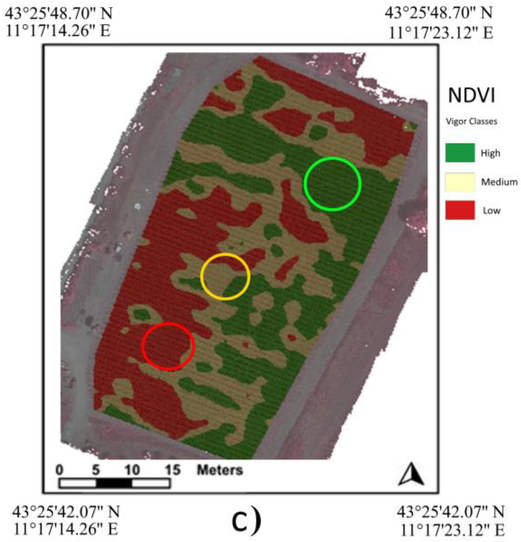
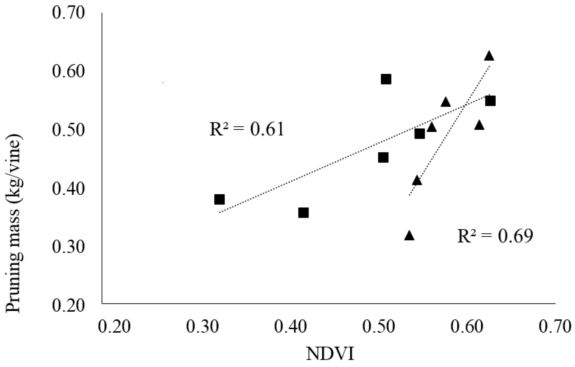
4.1. In-Field Vigor Variability

Figure 4 shows the distribution of homogeneous areas of NDVI with the filtered and unfiltered maps. Both highlight a high vigor area in the south that also extends eastwards. The area of low vigor is concentrated in the northern part of the vineyard mainly due to the land sloping downwards from north to south, resulting in different crop water availability. The two maps are similar and present only one difference in the north-west part where there is an extension of the high-vigor zone on the unfiltered map.
Table 3 highlights the difference in absolute NDVI value between unfiltered and filtered maps. The lower value in the unfiltered map is due to mixed pixels containing both canopy and soil. Results showed strong differences in shoot weights between the plants located in the low vigor (0.41 ± 0.05 kg/vine) and high vigor (0.56 ± 0.06 kg/vine) blocks. In these blocks, the NDVI values of the filtered and unfiltered maps were also extracted and compared with shoot weights, obtaining a good regression (Figure 5) that was higher in the filtered (R2 = 0.69) than unfiltered (R2 = 0.61) map. Bonilla et al. [30] performed correlation coefficients between NDVI and vegetative composition traits obtaining results from 0.5 to 0.73 in a Tempranillo vineyard. Filippetti et al. [31] found differences in pruning weight per meter of cordon of about 0.48 kg for low vigor (LV) and 1.17 Kg for high vigor (HV) in a Sangiovese vineyard. Gatti et al. [32] studied vegetative growth of Barbera grapevines as a function of vigor level with data averaged over 2012–2013 and found total pruning mass (kg/vine) of 0.485, 0.754 and 0.895 for LV, medium vigor (MV)and HV respectively. The present study confirms the high spatial variability in vineyard vegetative response and that NDVI is a good indicator of vine vigor, providing a rapid and effective tool for agronomic decisions such as site-specific canopy or soil management related to the real needs of the vines. For instance, a feasible option is that vineyard variability can be corrected according to the vigor level, achieving the best performance from variable rate fertilization as reported by Gatti et al. [32].

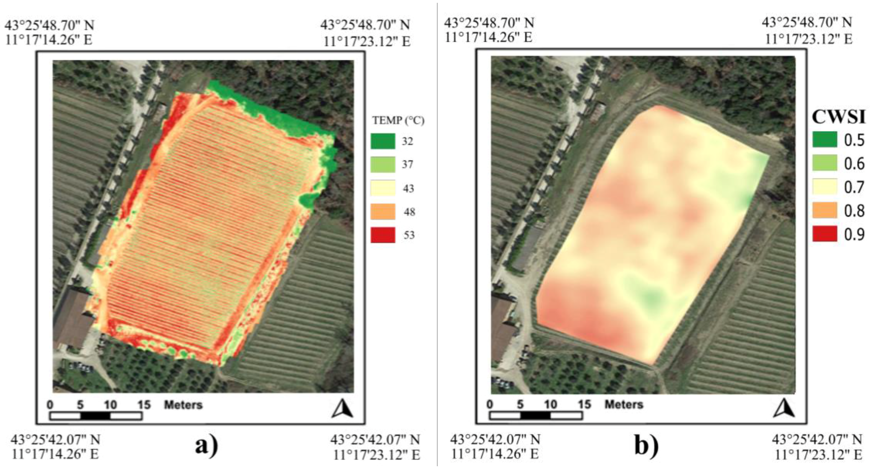
4.2. In-Field Thermal Variability and Crop Water Stress Index

Figure 3 presents the unfiltered temperature map (a) showing a temperature value for each pixel, and the interpolated CWSI map (b), produced after the canopy pure pixel filtering, in order to highlight the homogeneous areas of water stress. A wide range of CWSI values was found (0.5–0.9), confirming the relevance of within-field variability. Table 4 shows measured stomatal conductance and estimated CWSI at Site B for each vigor block. CWSI significantly increases from HV to LV, while stomatal conductance decreases thus confirming that water deficit induced an inhibition of photosynthesis caused by decreases in stomatal conductance.
Using low resolution thermal images, internal canopy shaded pixels often cannot be detected, leading to mixed information that negatively impacts the relationship between CWSI and water stress. The importance of UAV-based thermal images is the possibility of acquiring high resolution images that allow the filtering procedure to extract the pure canopy pixel temperature. The procedure used in this work was described in [31]. An interesting new filtering procedure based on the integration and automatic co-registration of thermal and multispectral images was described in [32]. The use of CWSI maps gives an advantage taking into account the spatial variability of vine water status with respect to time-consuming ground water stress measurements. It could be a useful approach for providing precision irrigation recommendations. For practical purposes, it would be necessary to replicate the measurements on several dates during the stress period to assess their consistency.

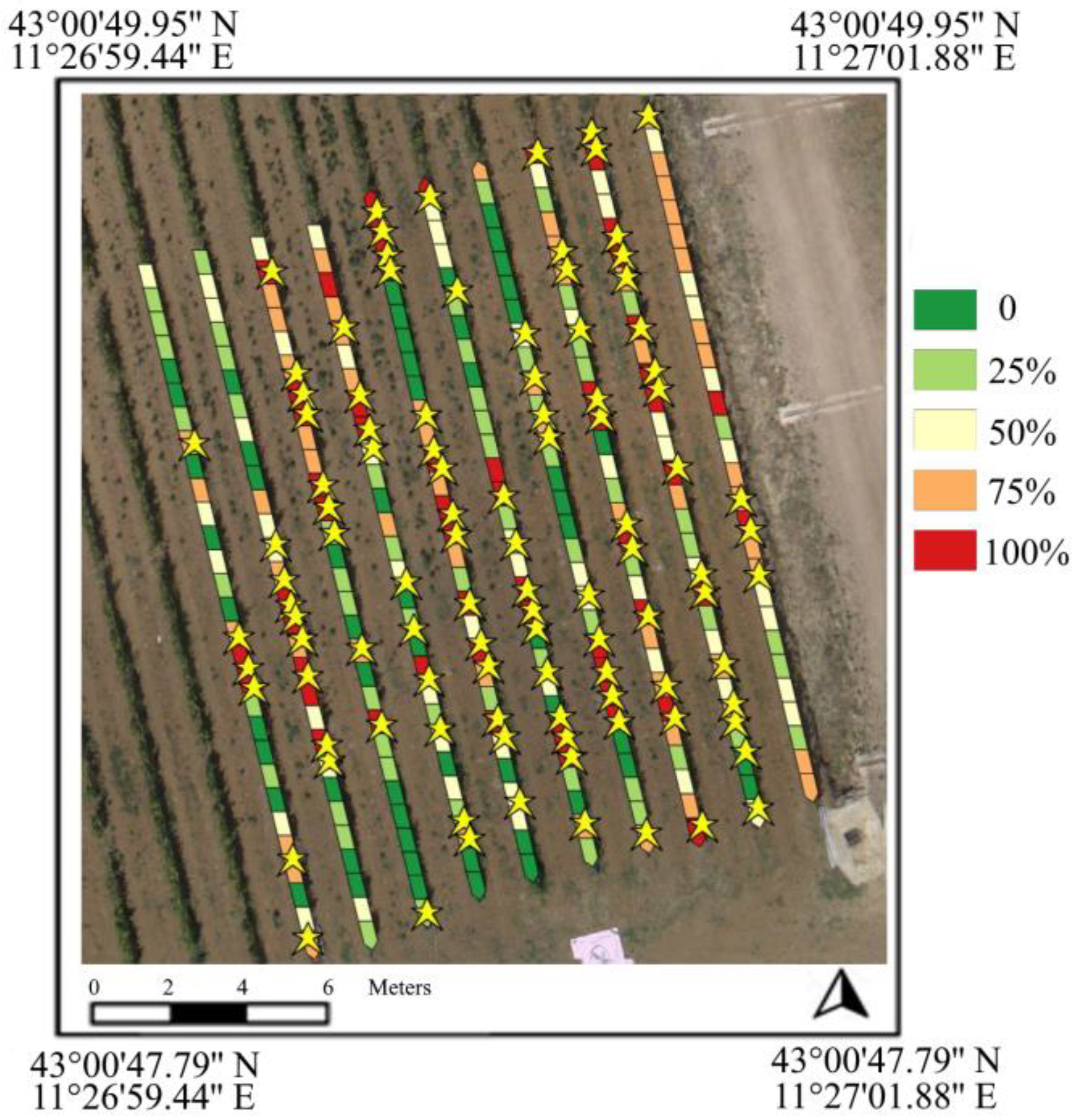
4.3. Missing Plant Monitoring

The map of missing plant classification is presented in Figure 6. The map indicates the missing plant positions (yellow stars) verified through ground observation at the end of the 2017 season. They were classified as level of potential missing plants: 100% (red), 75% (orange), 50% (yellow), 25% (light green) and no missing plants (dark green).
Table 5 shows the preliminary results obtained by elaboration of the remote sensing data and ground observations. The UAV method recognized 56 missing plants with 100% (red) and 27 with 75% (orange) accuracy; while it identified seven false negative missing plants, where a real missing plant is erroneously classified as a healthy plant. The table also presents the performance index of the proposed approach, calculated as the sum of red and orange classified plants divided by all missing plants detected by ground observation, according to the formula:
Performance Index = (RED + ORANGE)/Total missing plants (yellow stars) × 100
Observing the results, it emerges that the method tested at Site C identified 80% of total missing plants. Delenne et al. [33] developed a Fast Fourier Transform on an aerial image, providing the delineation of vineyards used to extract individual vine rows, with the aim of detecting missing plants and characterizing cultural practices, obtaining 90% of plots detected.
A critical analysis of the results, however, shows some negative performance indicators, such as “false positives”, i.e., plants erroneously estimated by drone as certain missing plants, indicated on the maps as red starless locations, whereas ground observation confirmed the absence of missing plants. There are also “false negatives”, i.e., positions erroneously estimated by drone as the presence of a plant (green), but from observation on the ground they are actually missing plants. Analyzing this aspect in detail, it is observed that the error in the UAV estimation does not concern the quality of the images or the correctness of elaboration, but green pixels related to the presence of weeds under the vine row. Specifically, the high presence of weeds on the row and the total or partial overlapping of adjacent plant shoots prevents the recognition of missing plants. The incorrect estimation of missing plants (false positives), however, is observed in situations where the canopy is much smaller than the majority of plants in the plot; this occurs either in conditions of very low vegetative vigor, or in the presence of recent replanting in which the cord has not yet been laid on the first thread and so there are large empty spaces between neighboring plants. The latter case is frequent in the eastern rows of the C site, recognizable on the map by many red polygons lacking the yellow star related to missing plants confirmed on the ground. While examples of plants with reduced vigor estimated as very probable (orange) missing plants were identified in the northern part of Site C.
The choice of period in which to do the survey is undoubtedly the most important factor; indeed, anticipating the flight by a few weeks it would have been possible to have plants with less vegetative development. Acquiring images with sprouts of about 0.30–0.40 m would undoubtedly have avoided canopy overlapping and full or partial coverage of missing plants. However, there might also have been the possibility of fewer weeds on the row.

4.4. Overall Evaluation

The article highlights the strengths of the work in terms of accuracy in describing the spatial variability of some ecophysiological traits in the vineyard using a UAV platform and validated with traditional ground measurements. Despite the fact that traditional ground measurements are a reference in terms of ground truth crop status, they are time-consuming and thereby to provide a representative number of measurements on large surfaces, becomes extremely difficult. Moreover, the UAV provides a rapid monitoring of large areas avoiding measurement errors caused by rapid alteration of microclimatic field conditions (air temperature, wind speed and radiation intensity).
From a critical analysis of the work described in this paper some weaknesses can be identified that must be taken into consideration for future work.
First of all, the study was carried out in three different sites, presenting only one type of remote sensing data for each site while the system was able to monitor with the three sensors simultaneously (multispectral, thermal and RGB). The reason of presenting different sites with single sensor is due to the farmer request for each work and consequently the ground measurements in support of remote sensing data validation. A second point was the lack of a precise monitoring of other descriptive ground parameters related to plant status, soil, microclimate, yield and quality. In precision viticulture works, sampling and measurements on several parameters are very important, in order to provide sufficient input to carry out a more in-depth analysis to describe the spatial variability according to a multivariate approach. Finally, in regards to missing plant monitoring, the applied method has provided some cases of incorrect classification due to the limit of 2D images to discriminate the canopy from the ground vegetation cover. The implementation of a photogrammetric approach aimed at the generation of a Canopy Height Model described in a precedent work by the authors [2], would have allowed to easily discriminate the vegetation in the vineyard according to height.

5. Conclusions

In recent years, unmanned aerial vehicles (UAVs) have become widely used in remote sensing activities in the vineyard, allowing high flexibility of use, low operating costs and a very high spatial resolution. UAV platforms can provide images with a detail that discriminates the row from the inter-row and thus provide pure pixels of only foliage, as opposed to traditional platforms in which the pixels of higher dimensions incorporate both canopy and soil or grassing, thus altering the actual plant vigor or temperature. Bare soil has a negative effect on the vigor index, while weeds or grassing tend to increase the vigor represented by the NDVI index, in this way a pixel containing vigorous plants plus bare ground would describe a less than real situation, and incorrect maps would be generated. Moreover, using a thermal camera to measure leaf temperature, the mixed pixel with bare soil tends to increase the actual leaf temperature data. The innovative approach tested to recognize individual plants and discriminate a missing plant from weeds on the row requires not only an extremely high spatial resolution but also an adequate temporal planning that is a compromise between the presence of sufficient vegetation and minimal growth of weeds.
The methodological applications described in this work present excellent performances in the characterization of spatial variability in terms of vegetative vigor, water stress and missing plant detection. A critical analysis of the results highlighted some weaknesses to be explored and considered for future work.
The study tested the applicability of RGB, multispectral and thermal sensors for specific purposes. This platform could be considered one of the first steps in future vineyard agronomic management, where “digital viticulture” will become an operating standard for the optimization of both production and traceability.

Author Contributions

A.M. and S.F.D.G. contributed equally to this work.

Funding

This research received no external funding.

Acknowledgments

The authors would like to thank Sigma Ingegneria for technological contribution in the UAV platform development. Authors are also grateful to Case Basse Farm for hosting and funding the missing plants experiment and Yuri Romboli (GESAAF UNIFI) for missing plants ground detection.

Conflicts of Interest

The authors declare no conflict of interest.

References

  1. Arnó, J.; Martínez-Casasnovas, J.A.; Ribes-Dasi, M.; Rosell, J.R. Review. Precision Viticulture. Research topics, challenges and opportunities in site-specific vineyard management. Span. J. Agric. Res. 2009, 7, 779–790. [Google Scholar]
  2. Matese, A.; Di Gennaro, S.F.; Berton, A. Assessment of a Canopy Height Model (CHM) in a vineyard using UAV-based multispectral imaging. Int. J. Remote Sens. 2017, 38, 8–10. [Google Scholar] [CrossRef]
  3. Matese, A.; Di Gennaro, S.F.; Miranda, C.; Berton, A.; Santesteban, L. Evaluation of spectral-based and canopy-based vegetation indices from UAV and Sentinel 2 images to assess spatial variability and ground vine parameters. Adv. Anim. Biosci. 2017, 8, 817–822. [Google Scholar] [CrossRef]
  4. Di Gennaro, S.F.; Matese, A.; Gioli, B.; Toscano, P.; Zaldei, A.; Palliotti, A.; Genesio, L. Multisensor approach to assess vineyard thermal dynamics combining high-resolution unmanned aerial vehicle (UAV) remote sensing and wireless sensor network (WSN) proximal sensing. Sci. Hortic. 2017, 221, 83–87. [Google Scholar] [CrossRef]
  5. Rouse, J.W.; Haas, R.H.; Schell, J.A.; Deering, D.W. Monitoring vegetation systems in the great plains with ERTS. In Proceedings of the 3rdEarth Resources Technology Satellite Symposium, Ottawa, ON, Canada, 10–14 December 1973; pp. 309–317. [Google Scholar]
  6. Goel, N.S. Models of vegetation canopy reflectance and their use in estimation of biophysical parameters from reflectance data. Remote Sens. Rev. 1988, 4, 1–212. [Google Scholar] [CrossRef]
  7. Jacquemoud, S.; Bacour, C.; Poilve, H.; Frangi, J.P. Comparison of four radiative transfer models to simulate plant canopies reflectance: Direct and inverse model. Remote Sens. Environ. 2000, 74, 417–481. [Google Scholar] [CrossRef]
  8. Zarco-Tejada, P.J.; Miller, J.R.; Noland, T.L.; Mohammed, G.H.; Sampson, P.H. Scaling-up and model inversion methods with narrow band optical indices for chlorophyll content estimation in closed forest canopies with hyper-spectral data. IEEE Trans. Geosci. Remote Sens. 2001, 39, 1491–1507. [Google Scholar] [CrossRef]
  9. Hall, A.; Lamb, D.W.; Holzapfel, B.; Louis, J. Optical remote sensing applications for viticulture—A review. Aust. J. Grape Wine Res. 2002, 8, 36–47. [Google Scholar] [CrossRef]
  10. Hall, A.; Louis, J.; Lamb, D. Characterising and mapping vineyard canopy using high-spatial-resolution aerial multispectral images. Comput. Geosci. 2003, 29, 813–822. [Google Scholar] [CrossRef]
  11. Fiorillo, E.; Crisci, A.; De Filippis, T.; Di Gennaro, S.F.; Di Blasi, S.; Matese, A.; Primicerio, J.; Vaccari, F.P.; Genesio, L. Airborne high-resolution images for grape classification: Changes in correlation between technological and late maturity in a Sangiovese vineyard in Central Italy. Aust. J. Grape Wine Res. 2012, 18, 80–90. [Google Scholar] [CrossRef]
  12. Filippetti, I.; Allegro, G.; Valentini, G.; Pastore, C.; Colucci, E.; Intrieri, C. Influence of vigour on vine performance and berry composition of cv. Sangiovese (Vitis vinifera L.). J. Int. Sci. Vigne Vin 2013, 47, 21–33. [Google Scholar] [CrossRef]
  13. Gatti, M.; Garavani, A.; Vercesi, A.; Poni, S. Ground-truthing of remotely sensed within-field variability in a cv. Barbera plot for improving vineyard management. Aust. J. Grape Wine Res. 2017, 23, 399–408. [Google Scholar] [CrossRef]
  14. Johnson, L.F.; Roczen, D.E.; Youkhana, S.K.; Nemani, R.R.; Bosch, D.F. Mapping vineyard leaf area with multispectral satellite imagery. Comput. Electron. Agric. 2003, 38, 33–44. [Google Scholar] [CrossRef]
  15. Berni, J.A.; Zarco-Tejada, P.J.; Suárez, L.; Fereres, E. Thermal and narrowband multispectral remote sensing for vegetation monitoring from an unmanned aerial vehicle. IEEE Trans. Geosci. Remote Sens. 2009, 47, 722–738. [Google Scholar] [CrossRef] [Green Version]
  16. Matese, A.; Toscano, P.; Di Gennaro, S.F.; Genesio, L.; Vaccari, F.P.; Primicerio, J.; Belli, C.; Zaldei, A.; Bianconi, R.; Gioli, B. Intercomparison of UAV, aircraft and satellite remote sensing platforms for precision viticulture. Remote Sens. 2015, 7, 2971–2990. [Google Scholar] [CrossRef]
  17. Santesteban, L.G.; Di Gennaro, S.F.; Herrero-Langreo, A.; Miranda, C.; Royo, J.B.; Matese, A. High-resolution UAV-based thermal imaging to estimate the instantaneous and seasonal variability of plant water status within a vineyard. Agric. Water Manag. 2017, 183, 49–59. [Google Scholar] [CrossRef]
  18. Jones, H.G. Irrigation scheduling: Advantages and pitfalls of plant-based methods. J. Exp. Bot. 2004, 55, 2427–2436. [Google Scholar] [CrossRef] [PubMed]
  19. Grant, O.M.; Tronina, L.; Jones, H.G.; Chaves, M.M. Exploring thermal imaging variables for the detection of stress responses in grapevine under different irrigation regimes. J. Exp. Bot. 2007, 58, 815–825. [Google Scholar] [CrossRef] [PubMed]
  20. Möller, M.; Alchanatis, V.; Cohen, Y.; Meron, M.; Tsipris, J.; Naor, A.; Ostrovsky, V.; Sprintsin, M.; Cohen, S. Use of thermal and visible imagery for estimating crop water status of irrigated grapevine. J. Exp. Bot. 2007, 58, 827–838. [Google Scholar] [CrossRef] [PubMed]
  21. Gontia, N.K.; Tiwari, K.N. Development of crop water stress index of wheat crop for scheduling irrigation using infrared thermometry. Agric. Water Manag. 2008, 95, 1144–1152. [Google Scholar] [CrossRef]
  22. Jones, H.G.; Serraj, R.; Loveys, B.R.; Xiong, L.; Wheaton, A.; Price, A.H. Thermal infrared imaging of crop canopies for the remote diagnosis and quantification of plant responses to water stress in the field. Funct. Plant. Biol. 2009, 36, 978–979. [Google Scholar] [CrossRef]
  23. Romano, G.; Zia, S.; Spreer, W.; Sanchez, C.; Cairns, J.; Araus, J.L.; Müller, J. Use of thermography for high throughput phenotyping of tropical maize adaptation in water stress. Comput. Electron. Agric. 2011, 79, 67–74. [Google Scholar] [CrossRef]
  24. Alchanatis, V.; Cohen, Y.; Cohen, S.; Moller, M.; Sprinstin, M.; Meron, M.; Tsipris, J.; Saranga, Y.; Sela, E. Evaluation of different approaches for estimating and mapping crop water status in cotton with thermal imaging. Precis. Agric. 2010, 11, 27–41. [Google Scholar] [CrossRef]
  25. Rabatel, G.; Delenne, C.; Deshayes, M. A non-supervised approach using Gabor filters for vine plot detection in aerial images. Comput. Electron. Agric. 2008, 62, 159–168. [Google Scholar] [CrossRef]
  26. Kelcey, J.; Lucieer, A. Sensor correction of a 6-band multispectral imaging sensor for UAV remote sensing. Remote Sens. 2012, 4, 1462–1493. [Google Scholar] [CrossRef]
  27. Jones, H.G.; Vaughan, R.A. Remote Sensing of Vegetation: Principles, Techniques, and Applications; Oxford University Press: Oxford, UK, 2010; ISBN 9780199207794. [Google Scholar]
  28. Idso, S.B.; Jackson, R.D.; Pinter, P.J.; Reginato, R.J.; Hatfield, J.L. Normalizing the stress degree day parameter for environmental variability. Agric. Meteorol. 1981, 24, 45–55. [Google Scholar] [CrossRef]
  29. Jones, H.G.; Stoll, M.; Santos, T.; de Sousa, C.; Chaves, M.M.; Grant, O.M. Use of infrared thermography for monitoring stomatal closure in the field: Application to grapevine. J. Exp. Bot. 2002, 53, 2249–2260. [Google Scholar] [CrossRef] [PubMed]
  30. Bonilla, I.; Martinez de Toda, F.; Martínez-Casasnovas, J.A. Vine vigour, yield and grape quality assessment by airborne remote sensing over three years: Analysis of unexpected relationships in cv. Tempranillo. Span. J. Agric. Res. 2015, 13, 1–8. [Google Scholar] [CrossRef]
  31. Matese, A.; Baraldi, R.; Berton, A.; Cesaraccio, C.; Di Gennaro, S.F.; Duce, P.; Facini, O.; Mameli, M.G.; Piga, A.; Zaldei, A. Estimation of water stress in grapevines using proximal and remote sensing methods. Remote Sens. 2018, 10, 114. [Google Scholar] [CrossRef]
  32. Poblete, T.; Ortega-Farías, S.; Ryu, D. Automatic coregistration algorithm to remove canopy shaded pixels in UAV-borne thermal images to improve the estimation of crop water stress index of a drip-irrigated Cabernet sauvignon vineyard. Sensors 2018, 18, 397. [Google Scholar] [CrossRef] [PubMed]
  33. Delenne, C.; Durrieu, S.; Rabatel, G.; Deshayes, M. From pixel to vine parcel: A complete methodology for vineyard delineation and characterization using remote-sensing data. Comput. Electron. Agric. 2010, 70, 78–83. [Google Scholar] [CrossRef] [Green Version]
Figure 1. Location map. (a) Site A Chianti Classico; (b) Site B Chianti Classico; (c) Site C Montalcino.
Agriculture 08 00116 g001
Figure 2. UAV (unmanned aerial vehicle) platform used in all experimental sites.
Agriculture 08 00116 g002
Figure 3. (a) Temperature (TEMP), (b) Crop Water Stress Index (CWSI) and (c) normalized difference vegetation index (NDVI) vigor maps from data acquired at Site B.
Agriculture 08 00116 g003aAgriculture 08 00116 g003b
Figure 4. Site A NDVI maps obtained from unfiltered (a) and filtered (b) approach.
Agriculture 08 00116 g004
Figure 5. Regression between NDVI unfiltered (■) and NDVI filtered (▲) with pruning mass weight (kg/vine).
Agriculture 08 00116 g005
Figure 6. Map of missing plant classification. Level of potential missing plants: 100% (red), 75% (orange), 50% (yellow), 25% (light green) and no missing plants (dark green) at Site C.
Agriculture 08 00116 g006
Table 1. Experimental sites.
CharacteristicsSite ASite BSite C
Monitored traitVigorWater stressMissing plants
AreaChianti ClassicoChianti ClassicoMontalcino
Location43°25′41.20” N
11°16′15.56” E
43°25′44.06” N
11°17′17.62” E
43°00′49.95” N
11°27′01.88” E
Planting year200420081973
Surface (ha)6.51.42.4
CultivarSangioveseSangioveseSangiovese
Spacing (m)3.0 × 0.9 2.2 × 0.8 3.0 × 1.0
Row orientationNE-SWNW-SENE-SW
Training systemspur pruned cordonspur pruned cordonspur pruned cordon
Date/Time of flight4 August 2017 12:00 9 August 2017 12:0023 May 2017 12:30
Growth stagesVeraisonVeraisonFruit-set
Soilmedium limestone mixmedium limestone mixSilt and calcic
Average temperature12.1 °C12.1 °C12.4 °C
Annual rainfall826 mm826 mm691 mm
Table 2. UAV (unmanned aerial vehicle) camera specifications used in the three field campaigns.
CharacteristicsTetracam ADC SnapFLIR TAU II 320Canon EOS M 10
Monitored traitVigorWater stressMissing plants
Camera typemultispectralthermalRGB
SensorCMOS global shutterCMOS StandardCMOS APS-C
Resolution (pixels)1280 × 1024324 × 2565280 × 3528
Sensor photo detectors (Mp)1.30.118.6
Spectral bandsR-G-NIR (Near Infrared)LWIR (Long Wave Infrared)R-G-B
Spectral range (nm)520–9207500–13,500400–700
Lens (mm)8.41918.0
Dimensions (mm)75 × 59 × 3345 × 45 × 30109 × 67 × 32
Weight (g)9072503
Table 3. Pruning weight, NDVI unfiltered and NDVI filtered calculated for each block.
VigorPruning Weight (kg/vine)NDVI UnfilteredNDVI Filtered
LV (Low Vigor)0.41 ± 0.05 **0.40 ± 0.06 ***0.55 ± 0.03 ***
HV (High Vigor)0.56 ± 0.06 **0.54 ± 0.09 ***0.60 ± 0.05 ***
Values are the mean ± SD. Statistical difference was assessed by Student’s t-test: ** p <0.01; *** p <0.001; ns: non-significant.
Table 4. Stomatal conductance measured at Site B for each vigor block.
VigorStomatal Conductance (mmol H2O m−2 s−1)CWSI
LV (Low Vigor)84.4 ± 11.26 **0.85 ± 0.05 **
MV (Medium Vigor)151.8 ± 22.53 **0.71 ± 0.02 **
HV (High Vigor)176.8 ± 25.49 **0.65 ± 0.03 **
CWSI, crop water stress index. Values are the mean ± SD. Statistical difference was assessed by Student’s t-test: ** p <0.01; ns: non-significant.
Table 5. Missing plants observation (Ground vs. UAV).
Ground-TruthUAV Missing Plant Classification
FieldTotal100% (RED)75% (ORANGE)50% (YELLOW)False NegativePerformance Index
C103562713780%

