
Environmental Assessment of Potentially Toxic Elements Using Pollution Indices and Data-Driven Modeling in Surface Sediment of the Littoral Shelf of the Mediterranean Sea Coast and Gamasa Estuary, Egypt

 ,
,  ,
,  ,
,  ,
,  ,
,  ,
, 
Abstract
:1. Introduction
2. Materials and Methods
2.1. Study Site Description
2.2. Sample Gathering, Automated Inspection, and Quality Control
2.3. Pollution Assessment Indices
2.4. Data Analyses
2.5. Random Forest
2.6. Back-Propagation Neural Network (BPNN)
2.7. Model Evaluation
2.8. Analytical Dataset and Software
3. Results and Discussion
3.1. Elements in Sediment
3.2. Pollution Assessment Indices
3.2.1. Contamination Factor (CF)
3.2.2. Enrichment Factor (EF)
3.2.3. Geoaccumulation Index (Igeo)
3.2.4. Multielement Pollution Indices (Dc, PLI, RI)
3.3. Correlation Matrix
3.4. Multivariate Statistical Analysis
3.4.1. Cluster Analysis
3.4.2. Principal Component Analysis
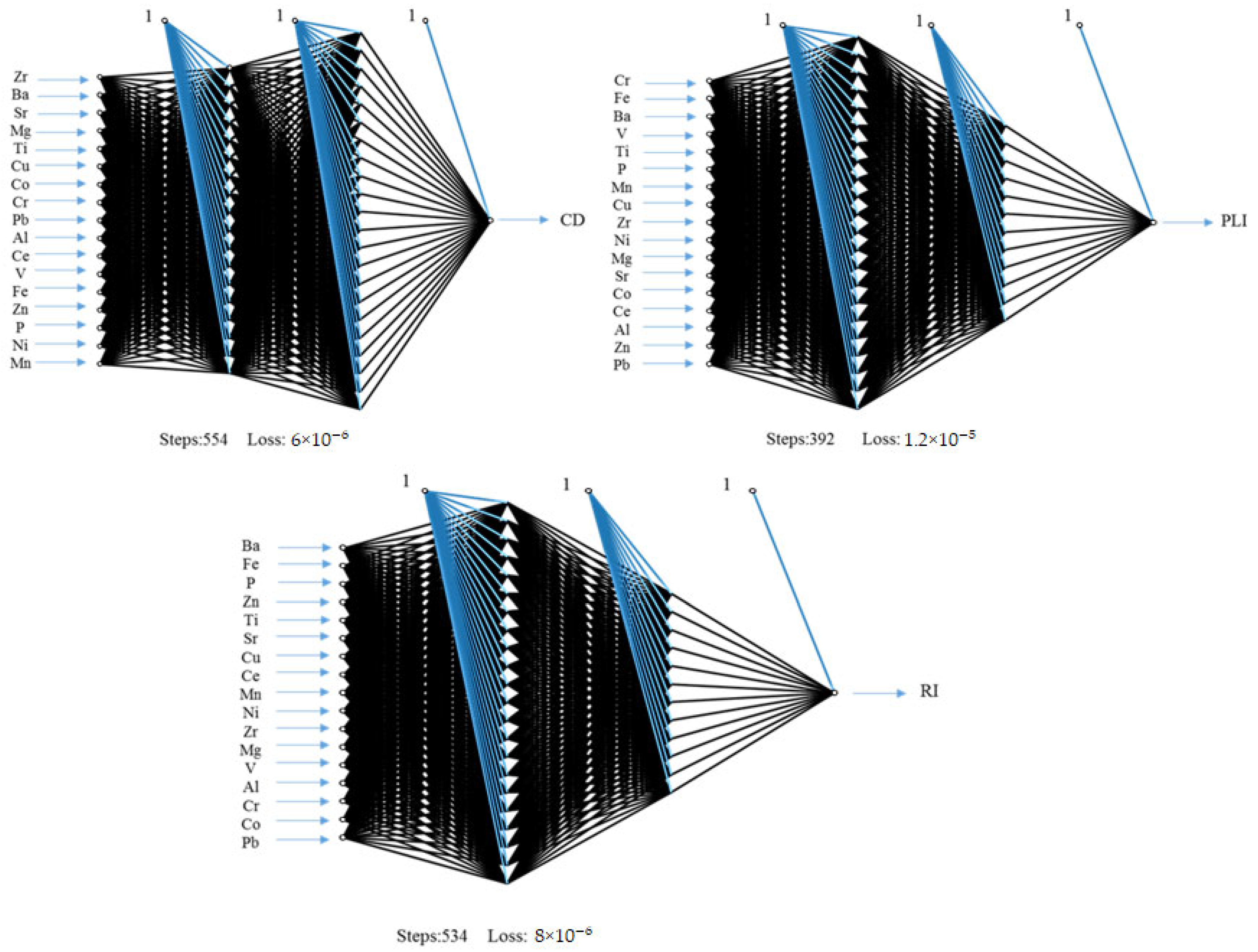
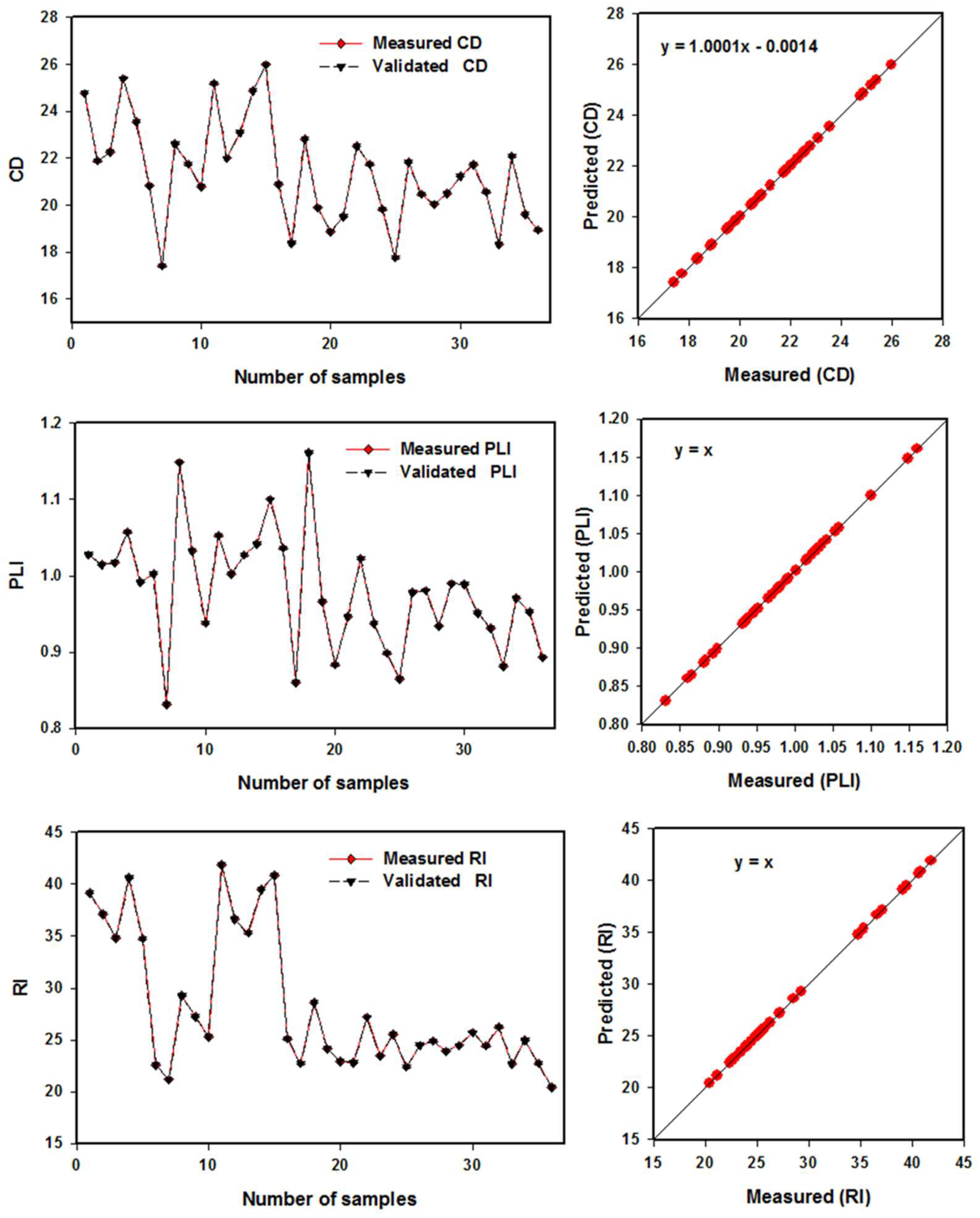
3.5. Performance of Random Forest and Artificial Neural Networks Based on Several Elements to Assess Pollution Indices
4. Conclusions
Supplementary Materials
Author Contributions
Funding
Data Availability Statement
Conflicts of Interest
References
- Green, A.J.; Planchart, A. The neurological toxicity of heavy metals: A fish perspective. Comp. Biochem. Physiol. C Toxicol. Pharmacol. 2018, 208, 12–19. [Google Scholar] [CrossRef] [PubMed]
- Sun, C.; Zhang, Z.; Cao, H.; Xu, M.; Xu, L. Concentrations, speciation, and ecological risk of heavy metals in the sediment of the Songhua River in an urban area with petrochemical industries. Chemosphere 2019, 219, 538–545. [Google Scholar] [CrossRef] [PubMed]
- Zhang, H.; Walker, T.R.; Davisa, E.; Ma, G. Ecological risk assessment of metals in small craft harbour sediments in Nova Scotia, Canada. Mar. Pollut. Bull. 2019, 146, 466–475. [Google Scholar] [CrossRef] [PubMed]
- Niu, Y.; Jiang, X.; Wang, K.; Xia, J.; Jiao, W.; Niu, Y.; Yu, H. Meta analysis of heavy metal pollution and sources in surface sediments of Lake Taihu, China. Sci. Total Environ. 2020, 700, 134509. [Google Scholar] [CrossRef] [PubMed]
- Abou El-Safa, M.M.; Gad, M.; Eid, E.M.; Alnemari, A.M.; Almarshadi, M.H.; Alshammari, A.S.; Moghanm, F.S.; Saleh, A.H. Environmental Risk Assessment of Petroleum Activities in Surface Sediments, Suez Gulf, Egypt. J. Mar. Sci. Eng. 2021, 9, 473. [Google Scholar] [CrossRef]
- Chen, H.; Wang, J.; Chen, J.; Lin, H.; Lin, C. Assessment of heavy metal contamination in the surface sediments: A reexamination into the offshore environment in China. Mar. Pollut. Bull. 2016, 113, 132–140. [Google Scholar] [CrossRef]
- Guo, B.; Liu, Y.; Zhang, F.; Hou, J.; Zhang, H.; Li, C. Heavy metals in the surface sediments of lakes on the Tibetan Plateau, China. Environ. Sci. Pollut. Res. 2018, 25, 3695–3707. [Google Scholar] [CrossRef]
- Pan, K.; Wang, W.X. Trace metal contamination in estuarine and coastal environments in China. Sci. Total Environ. 2012, 421, 3–16. [Google Scholar] [CrossRef]
- Pang, H.J.; Lou, Z.H.; Jin, A.M.; Yan, K.K.; Jiang, Y.; Yang, X.H.; Chen, C.T.A.; Chen, X.G. Contamination, distribution, and sources of heavy metals in the sediments of Andong tidal flat, Hangzhou Bay, China. Cont. Shelf Res. 2015, 110, 72–84. [Google Scholar] [CrossRef]
- Wardhani, E.; Rossmini, D.; Notodarmojo, S. Status of heavy metal in sediment of Saguling Lake, West Java. IOP Conf. Ser. Earth Environ. Sci. 2017, 60, 012035. [Google Scholar] [CrossRef] [Green Version]
- Szydłowski, K.; Rawicki, K.; Burczyk, P. The content of heavy metals in bottom sediments of the watercourse in agricultural catchment on the example of the river Gowienica. Inżynieria Ekol. 2017, 18, 218–224. [Google Scholar] [CrossRef]
- Tytła, M.; Kostecki, M. Ecological risk assessment of metals and metalloid in bottom sediments of water reservoir located in the key anthropogenic “hot spot” area (Poland). Environ. Earth Sci. 2019, 78, 179. [Google Scholar] [CrossRef] [Green Version]
- Masria, A.; Negm, A.; Iskander, M.; Saavedra, O. Coastal zone issues: A case study (Egypt). Procedia Eng. 2014, 70, 1102–1111. [Google Scholar] [CrossRef] [Green Version]
- Zhang, M.; He, P.; Qiao, G.; Huang, J.; Yuan, X.; Li, Q. Heavy metal contamination assessment of surface sediments of the Subei Shoal, China: Spatial distribution, source apportionment and ecological risk. Chemosphere 2019, 223, 211–222. [Google Scholar] [CrossRef] [PubMed]
- Vetrimurugan, E.; Shruti, V.C.; Jonathan, M.P.; Royd, P.D.; Sarkar, S.K.; Rawlins, B.K.; Villegas, L.E.C. Comprehensive study on metal contents and their ecological risks in beach sediments of KwaZulu-Natal province, South Africa. Mar. Pollut. Bull. 2019, 149, 110555. [Google Scholar] [CrossRef] [PubMed]
- Okbah, M.A.; Nasr, S.M.; Soliman, N.F.; Khairy, M.A. Distribution and Contamination Status of Trace Metals in the Mediterranean Coastal Sediments, Egypt. Soil Sediment Contam. Int. J. 2014, 23, 656–676. [Google Scholar] [CrossRef]
- Soliman, N.F.; Nasr, S.M.; Okbah, M.A. Potential ecological risk of heavy metals in sediments from the Mediterranean coast, Egypt. J. Environ. Health Sci. Eng. 2015, 13, 70. [Google Scholar] [CrossRef] [Green Version]
- El-Gamal, A.A.; Saleh, I.H. Geochemical Assessment of Heavy Metals Pollution and Ecological Risk in the Nile Delta Coastal Sediments, Egypt. J. King Abdulaziz Univ. Mar. Sci. 2016, 26, 41–59. [Google Scholar] [CrossRef]
- Abdallah, M.A.M.; Badr-ElDin, A.M. Ecological risk assessment of surficial sediment by heavy metals from a submerged archaeology harbor, South Mediterranean Sea, Egypt. Acta Geochim. 2020, 39, 226–235. [Google Scholar] [CrossRef]
- Khaled, A.; Ahdy, H.H.H.; Hamed, E.A.E.; Ahmed, H.O.; Abdel Razek, F.A.; Abdel Razek, M.A.; Elmasry, E. Spatial distribution and potential risk assessment of heavy metals in sediment along Alexandria Coast, Mediterranean Sea, Egypt. Egypt. J. Aquat. Res. 2021, 47, 37–43. [Google Scholar] [CrossRef]
- CAPMAS. The Central Agency for Public Mobilization and Statistics. The Arab Republic of Egypt. 2021. Available online: http://www.capmas.gov.eg/ (accessed on 22 April 2022).
- EEAA (Egyptian Environmental Affairs Agency). National Circumstances. Egypt Second National Communication on Climate Change. 2010. Available online: https://unfccc.int/resource/docs/natc/egync2.pdf (accessed on 22 April 2022).
- El-Sharnouby, B.A.; El-Alfy, K.S.; Rageh, O.S.; El-Sharabasy, M.M. Coastal Changes along Gamasa Beach, Egypt. J. Coast. Zone Manag. 2015, 18, 393. [Google Scholar] [CrossRef] [Green Version]
- Sarkar, A.; Pandey, P. River water quality modelling using artificial neural network technique. Aquat. Procedia 2015, 4, 1070–1077. [Google Scholar] [CrossRef]
- Isiyaka, H.A.; Mustapha, A.; Juahir, H.; Phil-Eze, P. Water quality modelling using artificial neural network and multivariate statistical techniques. Model Earth Syst. Environ. 2019, 5, 583–593. [Google Scholar] [CrossRef]
- Adnan, R.M.; Liang, Z.; El-Shafie, A.; Zounemat-Kermani, M.; Kisi, O. Daily streamflow prediction using optimally pruned extreme learning machine. J. Hydrol. 2019, 577, 123981. [Google Scholar] [CrossRef]
- Saleh, A.H.; Elsayed, S.; Gad, M.; Elmetwalli, A.H.; Elsherbiny, O.; Hussein, H.; Moghanm, F.S.; Qazaq, A.S.; Eid, E.M.; El-Kholy, A.S.; et al. Utilization of Pollution Indices, Hyperspectral Reflectance Indices, and Data-Driven Multivariate Modelling to Assess the Bottom Sediment Quality of Lake Qaroun, Egypt. Water 2022, 14, 890. [Google Scholar] [CrossRef]
- Šiljić Tomić, A.; Antanasijević, D.; Ristić, M.; Perić-Grujić, A.; Pocajt, V. Application of experimental design for the optimization of artificial neural network-based water quality model: A case study of dissolved oxygen prediction. Environ. Sci. Pollut. Res. Int. 2018, 25, 9360–9370. [Google Scholar] [CrossRef] [PubMed]
- Saleh, A.H.; Gad, M.; Khalifa, M.M.; Elsayed, S.; Moghanm, F.S.; Ghoneim, A.M.; Danish, S.; Datta, R.; Moustapha, M.E.; Abou El-Safa, M.M. Environmental Pollution Indices and Multivariate Modeling Approaches for Assessing the Potentially Harmful Elements in Bottom Sediments of Qaroun Lake, Egypt. J. Mar. Sci. Eng. 2021, 9, 1443. [Google Scholar] [CrossRef]
- Dorgham, M.; El-Tohamy, W.; Qin, J.; Abdel-Aziz, N.; El-Ghobashy, A. Mesozooplankton in a stressed area of the Nile Delta Coast, Egypt. Egypt. J. Aquat. Biol. Fish. 2019, 23, 89–105. [Google Scholar] [CrossRef] [Green Version]
- El-Gamal, A.A.; Saleh, I.H. Radiological and mineralogical investigation of accretion and erosion coastal sediments in Nile Delta Region, Egypt. J. Oceanogr. Mar. Sci. 2012, 3, 41–55. [Google Scholar] [CrossRef]
- US EPA (United States Environmental Protection Agency). Methods for Collection, Storage and Manipulation of Sediments for Chemical and Toxicological Analyses: Technical Manual; EPA-823-B-01-002; Office of Water: Washington, DC, USA, 2001.
- 2000a. E 1391-94; Standard Guide for Collection, Storage, Characterization, and Manipulation of Sediments for Toxicological Testing. ASTM: Conshohocken, PA, USA, 2000; Volume 11.05, pp. 768–788.
- US Environmental Protection Agency (EPA). Method 3052: Microwave Assisted Acid Digestion of Siliceous and Organically Based Matrices; Print Office: Washington, DC, USA, 1996; p. 20. [Google Scholar]
- Håkanson, L. An ecological risk index for aquatic pollution control: A sedimentological approach. Water Res. 1980, 14, 975–1003. [Google Scholar] [CrossRef]
- Guo, W.; Huo, S.; Xi, B.; Zhang, J.; Wub, F. Heavy metal contamination in sediments from typical lakes in the five geographic regions of China: Distribution, bioavailability, and risk. Ecol. Eng. 2015, 81, 243–255. [Google Scholar] [CrossRef]
- Wang, A.; Wei, C.; Xu, Y.; Hakif, M.; Hassan, A.; Ye, X.; Hoe, K. Assessment of heavy metal pollution in surficial sediments from a tropical river-estuary-shelf system: A case study of Kelantan River, Malaysia. Mar. Pollut. Bull. 2017, 125, 492–500. [Google Scholar] [CrossRef] [PubMed]
- Pekey, H. The distribution and sources of heavy metals in İzmit Bay surface sediments affected by a polluted stream. Mar. Pollut. Bull. 2006, 52, 1197–1208. [Google Scholar] [CrossRef] [PubMed]
- Abrahim, G.M.S.; Parker, R.J. Assessment of heavy metal enrichment factors and the degree of contamination in marine sediments from Tamaki Estuary, Auckland, New Zealand. Environ. Monit. Assess. 2008, 136, 227–238. [Google Scholar] [CrossRef] [PubMed]
- Varol, M.; Canpolat, Ö.; Eriş, K.K.; Çağlar, M. Trace metals in core sediments from a deep lake in eastern Turkey: Vertical concentration profiles, eco-environmental risks and possible sources. Ecotoxicol. Environ. Saf. 2020, 189, 110060. [Google Scholar] [CrossRef]
- Müller, G. Index of geoaccumulation in sediments of the Rhine River. GeoJournal 1969, 2, 108–118. [Google Scholar]
- Tiwari, M.; Sahu, S.K.; Bhangare, R.C.; Ajmal, P.Y.; Pandit, G.G. Depth profile of major and trace elements in estuarine core sediment using the EDXRF technique. Appl. Radiat. Isot. 2013, 80, 78–83. [Google Scholar] [CrossRef]
- Tomlinson, D.L.; Wilson, J.G.; Harris, C.R.; Jeffrey, D.W. Problems in the assessment of heavy-metal levels in estuaries and the formation of a pollution index. Helgoländer Meeresunters. 1980, 33, 566–575. [Google Scholar] [CrossRef] [Green Version]
- Harikumar, P.S.; Nasir, U.P.; Rahman, M.P.M. Distribution of heavy metals in the core sediments of a tropical wetland system. Int. J. Environ. Sci. Technol. 2009, 6, 225–232. [Google Scholar] [CrossRef] [Green Version]
- Maanan, M.; Saddik, M.; Maanan, M.; Chaibi, M. Environmental and ecological risk assessment of heavy metals in sediments of Nador lagoon, Morocco. Ecol. Indic. 2014, 48, 616–626. [Google Scholar] [CrossRef]
- Wang, C.; He, S.; Zou, Y.; Liu, J.; Zhao, R.; Yin, X.; Zhang, H.; Li, Y.W. Quantitative evaluation of in-situ bioremediation of compound pollution of oil and heavy metal in sediments from the Bohai Sea, China. Mar. Pollut. Bull. 2019, 150, 110787. [Google Scholar] [CrossRef] [PubMed]
- Cheng, W.H.; Yap, C.K. Potential human health risks from toxic metals via mangrove snail consumption and their ecological risk assessments in the habitat sediment from Peninsular Malaysia. Chemosphere 2015, 135, 156–165. [Google Scholar] [CrossRef] [PubMed]
- Looi, L.J.; Aris, A.Z.; Yusoff, F.M.; Isa, N.M.; Haris, H. Application of enrichment factor, geoaccumulation index, and ecological risk index in assessing the elemental pollution status of surface sediments. Environ. Geochem. Health 2019, 41, 27–42. [Google Scholar] [CrossRef]
- Zhuang, S.; Lu, X.; Yu, B.; Fan, X.; Yang, Y. Ascertaining the pollution, ecological risk and source of metal(loid)s in the upstream sediment of Danjiang River, China. Ecol. Indic. 2021, 125, 107502. [Google Scholar] [CrossRef]
- Hanif, N.; Eqani, S.A.M.A.S.; Ali, S.M.; Cincinelli, A.; Ali, N.; Katsoyiannis, I.A.; Bokhari, H. Geo-accumulation and enrichment of trace metals in sediments and their associated risks in the Chenab River, Pakistan. J. Geochem. Explor. 2016, 165, 62–70. [Google Scholar] [CrossRef]
- Jiang, D.; Wang, Y.; Zhou, S.; Long, Z.; Liao, Q.; Yang, J.; Fan, J. Multivariate analyses and human health assessments of heavy metals for surface water quality in the Xiangjiang River Basin, China. Environ. Toxicol. Chem. 2019, 38, 1645–1657. [Google Scholar] [CrossRef]
- Baran, A.; Tarnawski, M.; Koniarz, T. Spatial distribution of trace elements and ecotoxicity of bottom sediments in Rybnik reservoir, Silesian–Poland. Environ. Sci. Pollut. Res. Int. 2016, 23, 17255–17268. [Google Scholar] [CrossRef] [Green Version]
- Strobl, C.; Boulesteix, A.-L.; Kneib, T.; Augustin, T.; Zeileis, A. Conditional variable importance for random forests. BMC Bioinform. 2008, 9, 307. [Google Scholar] [CrossRef] [Green Version]
- Breiman, L. Random forests. Mach. Learn. 2001, 45, 5–32. [Google Scholar] [CrossRef] [Green Version]
- Schalkoff, J. Artificial Neural Networks; McGraw-Hill Companies Inc.: New York, NY, USA, 1997. [Google Scholar]
- Haykin, S. Neural Networks: A Comprehensive Foundation, 2nd ed.; Prentice Hall: Hoboken, NJ, USA, 1999. [Google Scholar]
- Li, J.; Yoder, R.; Odhiambo, L.O.; Zhang, J. Simulation of nitrate distribution under drip irrigation using artificial neural networks. Irrig. Sci. 2004, 23, 29–37. [Google Scholar] [CrossRef]
- Byrd, R.H.; Lu, P.; Nocedal, J.; Zhu, C. A limited memory algorithm for bound constrained optimization. Siam J. Sci. Comput. 1995, 16, 1190–1208. [Google Scholar] [CrossRef]
- Glorfeld, L.W. A methodology for simplification and interpretation of backpropagation-based neural network models. Expert Syst. Appl. 1996, 10, 37–54. [Google Scholar] [CrossRef]
- Malone, B.P.; Styc, Q.; Minasny, B.; McBratney, A.B. Digital soil mapping of soil carbon at the farm scale: A spatial downscaling approach in consideration of measured and uncertain data. Geoderma 2017, 290, 91–99. [Google Scholar] [CrossRef]
- Saggi, M.K.; Jain, S. Reference evapotranspiration estimation and modeling of the Punjab Northern India using deep learning. Comput. Electron. Agric. 2019, 156, 387–398. [Google Scholar] [CrossRef]
- Wang, C.; Nie, S.; Xi, X.H.; Luo, S.Z.; Sun, X.F. Estimating the biomass of maize with hyperspectral and LiDAR data. Remote Sen. 2017, 9, 11. [Google Scholar] [CrossRef] [Green Version]
- Zhu, J.; Huang, Z.H.; Sun, H.; Wang, G.X. Mapping forest ecosystem biomass density for Xiangjiang river basin by combining plot and remote sensing data and comparing spatial extrapolation methods. Remote Sens. 2017, 9, 241. [Google Scholar] [CrossRef] [Green Version]
- El Baz, S.M.; Khalil, M.M. Assessment of trace metals contamination in the coastal sediments of the Egyptian Mediterranean coast. J. Afr. Earth Sci. 2018, 143, 195–200. [Google Scholar] [CrossRef]
- Guen, C.; Tecchio, S.; Dauvin, J.; Roton, G.; Lobry, J.; Lepage, M.; Morin, J.; Lassalle, G.; Raoux, A.; Niquil, N. Assessing the ecological status of an estuarine ecosystem: Linking biodiversity and food-web indicators. Estuar. Coast Shelf Sci. 2019, 228, 106339. [Google Scholar] [CrossRef]
- Guo, C.; Chen, Y.; Xia, W.; Qu, X.; Yuan, H.; Xie, S.; Lin, L. Eutrophication and heavy metal pollution patterns in the water suppling lakes of China’s south-to-north water diversion project. Sci. Total Environ. 2020, 711, 134543. [Google Scholar] [CrossRef]
- Bantan, R.; Al-Dubai, T.; Al-Zubieri, A. Geo-environmental assessment of heavy metals in the bottom sediments of the Southern Corniche of Jeddah, Saudi Arabia. Mar. Pollut. Bull. 2020, 161, 111721. [Google Scholar] [CrossRef] [PubMed]
- Niu, L.; Li, J.; Luo, X.; Fu, T.; Chen, O.; Yang, O. Identification of heavy metal pollution in estuarine sediments under long-term reclamation: Ecological toxicity, sources and implications for estuary management. Environ. Pollut. 2021, 290, 118126. [Google Scholar] [CrossRef] [PubMed]
- Bai, J.; Xiao, R.; Cui, B.; Zhang, K.; Wang, Q.; Liu, X.; Gao, H.; Huang, L. Assessment of heavy metal pollution in wetland soils from the young and old reclaimed regions in the Pearl River Estuary, South China. Environ. Pollut. 2011, 159, 817–824. [Google Scholar] [CrossRef]
- Casado-Martínez, M.C.; Forja, J.M.; DelValls, T.A. A multivariate assessment of sediment contamination in dredged materials from Spanish ports. J. Hazard. Mater. 2009, 163, 1353–1359. [Google Scholar] [CrossRef] [PubMed]
- Paches, M.; Martínez-Guijarro, R.; Aguado, D.; Ferrer, J. Assessment of the impact of heavy metals in sediments along the Spanish Mediterranean coastline: Pollution indices. Environ. Sci. Pollut. Res. 2019, 26, 10887–10901. [Google Scholar] [CrossRef] [PubMed]
- El Nemr, A.M.; El Sikaily, A.; Khaled, A. Total and leachable heavy metals in muddy and sandy sediments of Egyptian coast along Mediterranean Sea. Environ. Monit. Assess. 2007, 129, 151–168. [Google Scholar] [CrossRef] [PubMed]
- Abdel Ghani, S.; El Zokm, G.; Shobier, A.; Othman, T.; Shreadah, M. Metal pollution in surface sediments of Abu-Qir Bay and Eastern Harbour of Alexandria, Egypt. Egypt. J. Aquat. Res. 2013, 39, 1–12. [Google Scholar] [CrossRef] [Green Version]
- El-Sorogy, A.S.; Tawfik, M.; Almadani, S.A.; Attiah, A. Assessment of toxic metals in coastal sediments of the Rosetta area, Mediterranean Sea, Egypt. Environ. Earth Sci. 2016, 75, 398. [Google Scholar] [CrossRef]
- Amor, R.B.; Yahyaoui, A.; Abidi, M.; Chouba, L.; Gueddari, M. Bioavailability and Assessment of Metal Contamination in Surface Sediments of Rades-Hamam Lif Coast, around Meliane River (Gulf of Tunis, Tunisia, Mediterranean Sea). J. Chem. 2019, 11, 4284987. [Google Scholar] [CrossRef]
- Chifflet, S.; Tedetti, M.; Zouch, H.; Fourati, R.; Zaghden, H.; Elleuch, B.; Quéméneur, M.; Karray, F.; Sayadi, S. Dynamics of trace metals in a shallow coastal ecosystem: Insights from the Gulf of Gabès (southern Mediterranean Sea). AIMS Environ. Sci. 2019, 6, 277–297. [Google Scholar] [CrossRef]
- Omar, M.B.; Mendiguchía, C.; Er-Raioui, H.; Marhraoui, M.; Lafraoui, G.; Oulad-Abdellah, M.K.; García-Vargas, M.; Moreno, C. Distribution of heavy metals in marine sediments of Tetouan coast (North of Morocco): Natural and anthropogenic sources. Environ. Earth Sci. 2015, 74, 4171–4185. [Google Scholar] [CrossRef]
- Díaz-de Alba, M.; Galindo-Riano, M.D.; Casanueva- Marenco, M.J.; Garcia-Vargas, M.; Kosore, C.M. Assessment of the metal pollution, potential toxicity and speciation of sediments from Algeciras Bay (South of Spain) using chemometric tools. J. Hazard. Mater. 2011, 190, 177–187. [Google Scholar] [CrossRef] [PubMed]
- Nour, H.E.; El-Sorogy, A.S. Distribution and enrichment of heavy metals in Sabratha coastal sediments, Mediterranean Sea, Libya. J. Afr. Earth Sci. 2017, 134, 222–229. [Google Scholar] [CrossRef]
- Merhaby, D.; Ouddane, B.; Net, S.; Halwani, J. Assessment of trace metals contamination in surficial sediments along Lebanese Coastal Zone. Mar. Pollut. Bull. 2018, 133, 881–890. [Google Scholar] [CrossRef] [PubMed]
- Choi, K.Y.; Kim, S.H.; Hong, G.H.; Chon, H.T. Distributions of heavy metals in the sediments of South Korean harbors. Environ. Geochem. Health 2012, 34, 71–82. [Google Scholar] [CrossRef]
- Diop, C.; Dewaelé, D.; Cazier, F.; Diouf, A.; Ouddane, B. Assessment of trace metals contamination level, bioavailability and toxicity in sediments from Dakar coast and Saint Louis estuary in Senegal, West Africa. Chemosphere 2015, 138, 980–987. [Google Scholar] [CrossRef] [PubMed]
- Duodu, G.O.; Goonetilleke, A.; Ayoko, G.A. Comparison of pollution indices for the assessment of heavy metal in Brisbane River sediment. Environ. Pollut. 2016, 219, 1077–1091. [Google Scholar] [CrossRef]
- Ahamad, M.I.; Song, J.; Sun, H.; Wang, X.; Mehmood, M.S.; Sajid, M.; Khan, A.J. Contamination level, ecological risk, and source identification of heavy metals in the hyporheic zone of the Weihe River, China. Int. J. Environ. Res. Public Health 2020, 17, 1070. [Google Scholar] [CrossRef] [Green Version]
- Jaskuła, J.; Sojka, M.; Fiedler, M.; Wróźyński, R. Analysis of Spatial Variability of River Bottom Sediment Pollution with Heavy Metals and Assessment of Potential Ecological Hazard for the Warta River, Poland. Minerals 2021, 11, 327. [Google Scholar] [CrossRef]
- Barik, S.K.; Muduli, P.R.; Mohanty, B.; Rath, P.; Samanta, S. Spatial distribution and potential biological risk of some metals in relation to granulometric content in core sediments from Chilika Lake, India. Environ. Sci. Pollut. Res. 2018, 25, 572–587. [Google Scholar] [CrossRef]
- Vineethkumar, V.; Sayooj, V.V.; Shimod, K.P.; Prakash, V. Estimation of pollution indices and hazard evaluation from trace elements concentration in coastal sediments of Kerala, Southwest Coast of India. Bull. Natl. Res. Cent. 2020, 44, 198. [Google Scholar] [CrossRef]
- Hronec, O.; Vilček, J.; Tomá, J.; Adamiin, P.; Huttmanová, E. Environmental Components Quality Problem Areas in Slovakia; Mendelova Univerzita: Brno, Czech Republic, 2010; 227p. [Google Scholar]
- Pavilonis, B.; Lioy, P.; Guazzetti, S.; Bostick, B.C.; Donna, F.; Peli, M.; Zimmerman, N.J.; Bertrand, P.; Lucas, E.; Smith, D.R.; et al. Manganese concentrations in soil and settled dust in an area with historic ferroalloy production. J. Expo. Sci. Environ. Epidemiol. 2015, 25, 443–450. [Google Scholar] [CrossRef] [PubMed] [Green Version]
- Adimalla, N.; Qian, H.; Wang, H. Assessment of heavy metal (HM) contamination in agricultural soil lands in northern Telangana, India: An approach of spatial distribution and multivariate statistical analysis. Environ. Monit. Assess. 2019, 191, 246. [Google Scholar] [CrossRef] [PubMed]
- Reimann, C.; Filzmoser, P.; Hron, K.; Kyňclová, P.; Garrett, R.G. A new method for correlation analysis of compositional (environmental) data-a worked example. Sci. Total Environ. 2017, 607, 965–971. [Google Scholar] [CrossRef]
- Zhang, J.; Zhou, F.; Chen, C.; Sun, X.; Shi, Y.; Zhao, H.; Chen, F. Spatial distribution and correlation characteristics of heavy metals in the seawater, suspended particulate matter and sediments in Zhanjiang Bay, China. PLoS ONE 2018, 13, e0201414. [Google Scholar] [CrossRef] [PubMed] [Green Version]
- Al-Wabel, M.I.; Sallam, A.E.-A.S.; Usman, A.R.A.; Ahmad, M.; El-Naggar, A.H.; El-Saeid, M.H.; Al-Faraj, A.; El-Enazi, K.; Al-Romian, F.A. Trace metal levels, sources, and ecological risk assessment in a densely agricultural area from Saudi Arabia. Environ. Monit. Assess. 2017, 189, 252. [Google Scholar] [CrossRef]
- Nazneen, S.; Singh, S.; Raju, N.J. Heavy metal fractionation in core sediments and potential biological risk assessment from Chilika lagoon, Odisha state, India. Quat. Int. 2019, 507, 370–388. [Google Scholar] [CrossRef]
- Elsayed, S.; Ibrahim, H.; Hussein, H.; Elsherbiny, O.; Elmetwalli, A.H.; Moghanm, F.S.; Ghoneim, A.M.; Danish, S.; Datta, R.; Gad, M. Assessment of water quality in Lake Qaroun using ground-based remote sensing data and artificial neural networks. Water 2021, 13, 3094. [Google Scholar] [CrossRef]
- Elsherbiny, O.; Fan, Y.; Zhou, L.; Qiu, Z. Fusion of Feature Selection Methods and Regression Algorithms for Predicting the Canopy Water Content of Rice Based on Hyperspectral Data. Agriculture 2021, 11, 51. [Google Scholar] [CrossRef]
- Thawornwong, S.; Enke, D. The adaptive selection of financial and economic variables for use with artificial neural networks. Neurocomputing 2004, 56, 205–232. [Google Scholar] [CrossRef]
- Melis, G.; Dyer, C.; Blunsom, P. On the state of the art of evaluation in neural language models. arXiv 2017, arXiv:1707.05589. [Google Scholar]
- Bergstra, J.; Yamins, D.; Cox, D. Making a Science of Model Search: Hyperparameter Optimization in Hundreds of Dimensions for Vision Architectures. In Proceedings of the 30th International Conference on Machine Learning (ICML 2013), Atlanta, GA, USA, 16–21 June 2013; pp. 115–123. [Google Scholar]
- Wu, J.; Chen, X.-Y.; Zhang, H.; Xiong, L.-D.; Lei, H.; Deng, S.-H. Hyperparameter optimization for machine learning models based on Bayesian optimization. J. Electron. Sci. Technol. 2019, 17, 26–40. [Google Scholar]
- Elsherbiny, O.; Zhou, L.; Feng, L.; Qiu, Z. Integration of Visible and Thermal Imagery with an Artificial Neural Network Approach for Robust Forecasting of Canopy Water Content in Rice. Remote Sens. 2021, 13, 1785. [Google Scholar] [CrossRef]
- Palani, S.; Liong, S.Y.; Tkalich, P. An ANN application for water quality forecasting. Mar. Pollut. Bull. 2008, 56, 1586–1597. [Google Scholar] [CrossRef] [PubMed]
- Ubah, J.I.; Orakwe, L.C.; Ogbu, K.N.; Awu, J.I.; Ahaneku, I.E.; Chukwuma, E.C. Forecasting water quality parameters using artificial neural network for irrigation purposes. Sci. Rep. 2021, 11, 24438. [Google Scholar] [CrossRef]


| Pollution Indices | Equation | Indices Criteria | Classes | Reference |
|---|---|---|---|---|
| CF | Mx: the potential toxic metal concentration in sediment samples. Mb: the concentration in the unpolluted “baseline” sediment (background value). | ≤1 | Low CF | [35] |
| 1 < CF ≤ 3 | Moderate CF | |||
| 3 < CF ≤ 6 | Considerable CF | |||
| 6 < CF | Very high | |||
| Dc | CF: the contamination factor of each analyzed element in the sample. i: the number of analyzed elements. | <8 | Low Dc | [35] |
| 8 < Dc < 16 | Moderate Dc | |||
| 16 < Dc < 32 | Considerable Dc | |||
| Dc > 32 | Very high Dc | |||
| EF | (Cx/CAl) sample: the metal to Al ratio in the tested sample. (Cx/CAl) background: the value of the metal to Al ratio in the natural background. | <1 | No enrichment | [49] |
| 1–3 | Minor enrichment | |||
| 3–5 | Moderate enrichment | |||
| 5–10 | Moderately severe enrichment | |||
| 10–25 | Severe enrichment | |||
| 25–50 | Very severe enrichment | |||
| ˃50 | Extremely severe enrichment | |||
| Igeo | Cn: the measured concentration of heavy metal n in the sampled sediment. Bn: the geochemical background of the element that is adapted from the literature. | Igeo ≤ 0 | Unpolluted | [41] |
| 0 < Igeo ≤ 1 | Unpolluted to Moderately polluted | |||
| 1 < Igeo ≤ 2 | Moderately polluted | |||
| 2 < Igeo ≤ 3 | Moderately to strongly polluted | |||
| 3 ˂ Igeo ≤ 4 | Strongly polluted | |||
| 4 < Igeo ≤ 5 | Strongly to extremely polluted | |||
| 5 < Igeo | Extremely polluted | |||
| PLI | PLI = (CF1 × CF2 × CF3 ×…× CFn)1/n | 1 > PLI | Unpolluted | [44] |
| 1 < PLI | Polluted | |||
| RI | Er: the potential ecological risk factor of an individual element. Tr: the toxic response factor. CF: the contamination factor. | RI < 150 | Low ecological risk | [35] |
| 150 < RI < 300 | Moderate ecological risk | |||
| 300 < RI < 600 | Considerable ecological risk | |||
| 600 < RI | Very high ecological risk |
| Elements | First Year (n = 54) | Second Year (n = 54) | Across Two Years (n = 108) | ||||||||||||||||
|---|---|---|---|---|---|---|---|---|---|---|---|---|---|---|---|---|---|---|---|
| Estuary | Littoral | Estuary | Littoral | Estuary | Littoral | ||||||||||||||
| Min | Max | Mean | Min | Max | Mean | Min | Max | Mean | Min | Max | Mean | Min | Max | Mean | Min | Max | Mean | ||
| Al | (%) | 3.69 | 7.71 | 4.95 | 4.20 | 4.90 | 4.47 | 3.69 | 7.57 | 4.96 | 4.17 | 4.95 | 4.47 | 3.69 | 7.71 | 4.95 | 4.17 | 4.95 | 4.47 |
| Fe | 2.34 | 5.12 | 3.24 | 3.14 | 4.49 | 4.04 | 2.39 | 5.14 | 3.25 | 3.26 | 4.47 | 4.03 | 2.34 | 5.14 | 3.25 | 3.14 | 4.49 | 4.03 | |
| Ti | 0.47 | 0.86 | 0.60 | 0.71 | 0.79 | 0.76 | 0.46 | 0.84 | 0.60 | 0.72 | 0.79 | 0.76 | 0.46 | 0.86 | 0.60 | 0.71 | 0.79 | 0.76 | |
| Mn | 0.24 | 0.51 | 0.37 | 0.18 | 0.28 | 0.23 | 0.28 | 0.50 | 0.37 | 0.18 | 0.29 | 0.23 | 0.24 | 0.51 | 0.37 | 0.18 | 0.29 | 0.23 | |
| Mg | 1.01 | 1.97 | 1.48 | 1.81 | 2.10 | 1.95 | 1.33 | 1.83 | 1.47 | 1.86 | 2.29 | 1.98 | 1.01 | 1.97 | 1.48 | 1.81 | 2.29 | 1.96 | |
| P | 0.12 | 0.16 | 0.14 | 0.06 | 0.08 | 0.07 | 0.10 | 0.17 | 0.13 | 0.06 | 0.08 | 0.07 | 0.10 | 0.17 | 0.14 | 0.06 | 0.08 | 0.07 | |
| V | (ppm) | 115 | 163 | 130 | 162 | 250 | 202 | 116 | 151 | 130 | 182 | 234 | 205 | 115 | 163 | 130 | 162 | 250 | 203 |
| Cr | 115 | 162 | 138 | 142 | 290 | 232 | 101 | 159 | 138 | 170 | 273 | 222 | 101 | 162 | 138 | 142 | 290 | 227 | |
| Co | 13.0 | 27.0 | 20.7 | 18.0 | 24.0 | 21.8 | 11.0 | 35.0 | 21.3 | 17.0 | 26.0 | 21.5 | 11.0 | 35.0 | 21.0 | 17.0 | 26.0 | 21.6 | |
| Ni | 22.0 | 38.0 | 29.3 | 28.0 | 39.0 | 33.0 | 22.0 | 35.0 | 29.4 | 30.0 | 36.0 | 33.4 | 22.0 | 38.0 | 29.3 | 28.0 | 39.0 | 33.2 | |
| Cu | 19.0 | 33.0 | 27.4 | 11.0 | 16.0 | 12.8 | 20.0 | 34.0 | 28.5 | 8.00 | 15.0 | 11.9 | 19.0 | 34.0 | 28.0 | 8.00 | 16.0 | 12.3 | |
| Zn | 97.0 | 132 | 113 | 36.0 | 59.0 | 46.6 | 75.0 | 129 | 107 | 31.0 | 65.0 | 46.1 | 75.0 | 132 | 110 | 31.0 | 65.0 | 46.4 | |
| Sr | 191 | 263 | 223 | 242 | 294 | 269 | 184 | 270 | 223 | 241 | 300 | 270 | 184 | 270 | 223 | 241 | 300 | 269 | |
| Ba | 266 | 501 | 399 | 202 | 301 | 253 | 217 | 520 | 395 | 189 | 293 | 252 | 217 | 520 | 397 | 189 | 301 | 252 | |
| Pb | 5.00 | 30.0 | 16.3 | 2.00 | 6.00 | 4.88 | 6.0 | 30.0 | 17.0 | 3.00 | 6.00 | 5.13 | 5.00 | 30.0 | 16.7 | 2.00 | 6.00 | 5.00 | |
| Zr | 149 | 258 | 185 | 240 | 383 | 319 | 139 | 274 | 192 | 221 | 389 | 321 | 139 | 274 | 189 | 221 | 389 | 320 | |
| Ce | 17.0 | 42.0 | 28.6 | 23.0 | 72.0 | 52.6 | 16.0 | 47.0 | 29.0 | 31.0 | 75.0 | 52.6 | 16.0 | 47.0 | 28.8 | 23.0 | 75.0 | 52.6 | |
| Region | Country | Al | Fe | Ti | Mn | Mg | P | V | Cr | Co | Ni | Cu | Zn | Sr | Ba | Pb | Zr | Ce | Reference |
|---|---|---|---|---|---|---|---|---|---|---|---|---|---|---|---|---|---|---|---|
| Estuary | Egypt | 49,500 | 32,500 | 6000 | 3700 | 14,800 | 1400 | 130 | 138 | 21.0 | 29.3 | 28.0 | 110 | 223 | 397 | 16.7 | 189 | 28.8 | Present study |
| Littoral shelf | 44,700 | 40,300 | 7600 | 2300 | 19,600 | 700 | 203 | 227 | 21.6 | 33.2 | 12.3 | 46.4 | 269 | 252 | 5.00 | 320 | 52.6 | ||
| Mediterranean coast | - | 13,256 | - | 381.0 | - | - | - | 82.74 | 8.24 | 25.93 | 8.46 | 22.19 | - | - | 13.17 | - | - | [17] | |
| Alexandria | - | 93,145 | - | 469.19 | - | - | - | 58.25 | 39.2 | 71.2 | 41.71 | 75.31 | 92.93 | - | - | [72] | |||
| Abu-Qir Bay | 9424 | 15,904 | - | 233.37 | - | - | 22.66 | - | - | - | 13.64 | 50.93 | 8.2 | - | - | [73] | |||
| Eastern Harbor | 2167 | - | - | - | - | - | - | 9.86 | - | - | - | - | 81.1 | - | - | [19] | |||
| Mediterranean coast | - | 13,256 | - | 381.0 | - | - | - | 82.74 | 8.24 | 25.93 | 8.46 | 22.19 | 13.17 | - | - | [16] | |||
| Mediterranean coast | - | 17,175 | - | 553.2 | - | - | - | - | - | - | 11.3 | 27.2 | - | - | 14.75 | - | - | [64] | |
| Rosetta coast | - | 109,560 | - | 553 | 510 | 1539 | 375 | 0.18 | 69.8 | 481 | 24.6 | 183 | - | - | 384 | - | - | [74] | |
| Rades-Hamam Lif Coast | Tunis | - | - | - | - | - | - | - | 30.14 | - | 22.71 | 24.37 | 72.78 | - | - | 35.78 | - | - | [75] |
| Gulf of Gabès | - | 5827 | - | 85.67 | - | - | 25.24 | 31.97 | 2.4 | 8.21 | 7.05 | 44.20 | - | - | 8.31 | - | - | [76] | |
| Tetouan coast | Morocco | 33,800 | 39,700 | -- | 362.86 | - | - | - | 128.39 | 23.24 | 50.28 | 14.88 | 84.26 | - | - | 41.11 | - | - | [77] |
| Algeciras Bay | Spain | - | 28,129 | - | 534 | - | - | 36.0 | 112.0 | 11.0 | 65.0 | 17.0 | 73.0 | - | - | 24.0 | - | - | [78] |
| Mediterranean coastline | - | - | - | - | - | - | - | 15.07 | - | 7.73 | 3.29 | 30.6 | - | - | 5.7 | - | - | [71] | |
| Sabratha | Libya | - | 2084 | - | 36.21 | - | - | - | - | 5.59 | 22.65 | 17.3 | 26.55 | - | - | 11.69 | - | - | [79] |
| Mediterranean coastline | Lebanon | - | - | - | 247 | - | - | 58.2 | 49.5 | 3.36 | 27.2 | - | 128 | - | - | 98.26 | - | - | [80] |
| Elements | First Year (n = 54) | Second Year (n = 54) | Across Two Years (n = 108) | |||||||||||||||
|---|---|---|---|---|---|---|---|---|---|---|---|---|---|---|---|---|---|---|
| Estuary | Littoral | Estuary | Littoral | Estuary | Littoral | |||||||||||||
| Min | Max | Mean | Min | Max | Mean | Min | Max | Mean | Min | Max | Mean | Min | Max | Mean | Min | Max | Mean | |
| Al | 0.46 | 0.96 | 0.62 | 0.52 | 0.61 | 0.56 | 0.46 | 0.94 | 0.62 | 0.52 | 0.62 | 0.56 | 0.46 | 0.96 | 0.62 | 0.52 | 0.62 | 0.56 |
| Fe | 0.67 | 1.46 | 0.93 | 0.90 | 1.28 | 1.15 | 0.68 | 1.47 | 0.93 | 0.93 | 1.28 | 1.15 | 0.67 | 1.47 | 0.93 | 0.90 | 1.28 | 1.15 |
| Ti | 0.94 | 1.72 | 1.20 | 1.42 | 1.58 | 1.51 | 0.91 | 1.68 | 1.20 | 1.44 | 1.58 | 1.52 | 0.91 | 1.72 | 1.20 | 1.42 | 1.58 | 1.51 |
| Mn | 4.00 | 8.50 | 6.17 | 3.00 | 4.67 | 3.76 | 4.65 | 8.39 | 6.20 | 3.07 | 4.91 | 3.78 | 4.00 | 8.50 | 6.18 | 3.00 | 4.91 | 3.77 |
| Mg | 0.44 | 0.86 | 0.64 | 0.79 | 0.91 | 0.85 | 0.58 | 0.80 | 0.64 | 0.81 | 0.99 | 0.86 | 0.44 | 0.86 | 0.64 | 0.79 | 0.99 | 0.85 |
| P | 1.09 | 1.45 | 1.26 | 0.55 | 0.72 | 0.63 | 0.87 | 1.52 | 1.23 | 0.57 | 0.73 | 0.64 | 0.87 | 1.52 | 1.24 | 0.55 | 0.73 | 0.64 |
| V | 1.11 | 1.57 | 1.25 | 1.56 | 2.40 | 1.95 | 1.12 | 1.45 | 1.25 | 1.75 | 2.25 | 1.97 | 1.11 | 1.57 | 1.25 | 1.56 | 2.40 | 1.96 |
| Cr | 1.35 | 1.91 | 1.63 | 1.67 | 3.41 | 2.73 | 1.19 | 1.87 | 1.63 | 2.00 | 3.21 | 2.61 | 1.19 | 1.91 | 1.63 | 1.67 | 3.41 | 2.67 |
| Co | 0.76 | 1.59 | 1.22 | 1.06 | 1.41 | 1.28 | 0.65 | 2.06 | 1.26 | 1.00 | 1.53 | 1.27 | 0.65 | 2.06 | 1.24 | 1.00 | 1.53 | 1.27 |
| Ni | 0.44 | 0.76 | 0.59 | 0.56 | 0.78 | 0.66 | 0.44 | 0.70 | 0.59 | 0.60 | 0.72 | 0.67 | 0.44 | 0.76 | 0.59 | 0.56 | 0.78 | 0.66 |
| Cu | 0.76 | 1.32 | 1.10 | 0.44 | 0.64 | 0.51 | 0.80 | 1.36 | 1.14 | 0.32 | 0.60 | 0.48 | 0.76 | 1.36 | 1.12 | 0.32 | 0.64 | 0.49 |
| Zn | 1.37 | 1.86 | 1.60 | 0.51 | 0.83 | 0.66 | 1.06 | 1.82 | 1.50 | 0.44 | 0.92 | 0.65 | 1.06 | 1.86 | 1.55 | 0.44 | 0.92 | 0.65 |
| Sr | 0.51 | 0.70 | 0.60 | 0.65 | 0.78 | 0.72 | 0.49 | 0.72 | 0.59 | 0.64 | 0.80 | 0.72 | 0.49 | 0.72 | 0.59 | 0.64 | 0.80 | 0.72 |
| Ba | 0.53 | 1.00 | 0.80 | 0.40 | 0.60 | 0.51 | 0.43 | 1.04 | 0.79 | 0.38 | 0.59 | 0.51 | 0.43 | 1.04 | 0.79 | 0.38 | 0.60 | 0.51 |
| Pb | 0.31 | 1.88 | 1.02 | 0.13 | 0.38 | 0.31 | 0.38 | 1.88 | 1.06 | 0.19 | 0.38 | 0.32 | 0.31 | 1.88 | 1.04 | 0.13 | 0.38 | 0.31 |
| Zr | 0.90 | 1.56 | 1.12 | 1.45 | 2.32 | 1.94 | 0.84 | 1.66 | 1.17 | 1.34 | 2.36 | 1.94 | 0.84 | 1.66 | 1.14 | 1.34 | 2.36 | 1.94 |
| Ce | 0.24 | 0.60 | 0.41 | 0.33 | 1.03 | 0.75 | 0.23 | 0.67 | 0.41 | 0.44 | 1.07 | 0.75 | 0.23 | 0.67 | 0.41 | 0.33 | 1.07 | 0.75 |
| Elements | First Year (n = 54) | Second Year (n = 54) | Across Two Years (n = 108) | |||||||||||||||
|---|---|---|---|---|---|---|---|---|---|---|---|---|---|---|---|---|---|---|
| Estuary | Littoral | Estuary | Littoral | Estuary | Littoral | |||||||||||||
| Min | Max | Mean | Min | Max | Mean | Min | Max | Mean | Min | Max | Mean | Min | Max | Mean | Min | Max | Mean | |
| Al | 1.00 | 1.00 | 1.00 | 1.00 | 1.00 | 1.00 | 1.00 | 1.00 | 1.00 | 1.00 | 1.00 | 1.00 | 1.00 | 1.00 | 1.00 | 1.00 | 1.00 | 1.00 |
| Fe | 1.06 | 1.87 | 1.49 | 1.63 | 2.43 | 2.08 | 1.05 | 1.78 | 1.50 | 1.72 | 2.46 | 2.08 | 1.05 | 1.87 | 1.50 | 1.63 | 2.46 | 2.08 |
| Ti | 1.50 | 2.54 | 2.01 | 2.53 | 3.02 | 2.72 | 1.57 | 2.63 | 2.00 | 2.48 | 3.04 | 2.73 | 1.50 | 2.63 | 2.00 | 2.48 | 3.04 | 2.73 |
| Mn | 4.52 | 18.0 | 11.1 | 5.46 | 8.30 | 6.77 | 4.94 | 17.8 | 11.2 | 5.66 | 8.18 | 6.79 | 4.52 | 18.0 | 11.2 | 5.46 | 8.30 | 6.78 |
| Mg | 0.70 | 1.32 | 1.09 | 1.36 | 1.75 | 1.53 | 0.80 | 1.39 | 1.10 | 1.39 | 1.90 | 1.55 | 0.70 | 1.39 | 1.10 | 1.36 | 1.90 | 1.54 |
| P | 1.52 | 2.60 | 2.15 | 0.99 | 1.37 | 1.14 | 1.34 | 2.69 | 2.10 | 1.02 | 1.24 | 1.14 | 1.34 | 2.69 | 2.13 | 0.99 | 1.37 | 1.14 |
| V | 1.50 | 2.62 | 2.12 | 2.73 | 4.60 | 3.51 | 1.54 | 2.73 | 2.13 | 3.03 | 4.34 | 3.55 | 1.50 | 2.73 | 2.13 | 2.73 | 4.60 | 3.53 |
| Cr | 1.48 | 4.08 | 2.90 | 2.93 | 6.44 | 4.94 | 1.54 | 4.08 | 2.88 | 3.40 | 6.13 | 4.72 | 1.48 | 4.08 | 2.89 | 2.93 | 6.44 | 4.83 |
| Co | 0.91 | 3.08 | 2.15 | 1.93 | 2.68 | 2.31 | 0.99 | 4.22 | 2.27 | 1.84 | 2.83 | 2.28 | 0.91 | 4.22 | 2.21 | 1.84 | 2.83 | 2.29 |
| Ni | 0.62 | 1.35 | 1.00 | 0.92 | 1.48 | 1.19 | 0.59 | 1.53 | 1.01 | 0.97 | 1.31 | 1.20 | 0.59 | 1.53 | 1.01 | 0.92 | 1.48 | 1.20 |
| Cu | 0.91 | 2.88 | 1.94 | 0.72 | 1.23 | 0.92 | 1.08 | 2.89 | 2.02 | 0.54 | 1.10 | 0.86 | 0.91 | 2.89 | 1.98 | 0.54 | 1.23 | 0.89 |
| Zn | 1.59 | 3.83 | 2.84 | 0.96 | 1.51 | 1.18 | 1.42 | 3.81 | 2.68 | 0.81 | 1.69 | 1.18 | 1.42 | 3.83 | 2.76 | 0.81 | 1.69 | 1.18 |
| Sr | 0.73 | 1.14 | 1.00 | 1.12 | 1.44 | 1.29 | 0.72 | 1.18 | 1.00 | 1.15 | 1.41 | 1.30 | 0.72 | 1.18 | 1.00 | 1.12 | 1.44 | 1.29 |
| Ba | 0.85 | 2.19 | 1.42 | 0.74 | 1.08 | 0.91 | 0.67 | 2.26 | 1.41 | 0.73 | 1.08 | 0.91 | 0.67 | 2.26 | 1.41 | 0.73 | 1.08 | 0.91 |
| Pb | 0.39 | 4.09 | 2.01 | 0.24 | 0.71 | 0.55 | 0.50 | 4.09 | 2.06 | 0.36 | 0.69 | 0.58 | 0.39 | 4.09 | 2.04 | 0.24 | 0.71 | 0.56 |
| Zr | 1.24 | 2.68 | 1.89 | 2.56 | 4.44 | 3.49 | 1.35 | 3.40 | 1.98 | 2.32 | 4.55 | 3.52 | 1.24 | 3.40 | 1.94 | 2.32 | 4.55 | 3.51 |
| Ce | 0.52 | 0.80 | 0.65 | 0.62 | 1.95 | 1.36 | 0.50 | 0.83 | 0.66 | 0.77 | 1.97 | 1.36 | 0.50 | 0.83 | 0.66 | 0.62 | 1.97 | 1.36 |
| Elements | First Year (n = 54) | Second Year (n = 54) | Across Two Years (n = 108) | |||||||||||||||
|---|---|---|---|---|---|---|---|---|---|---|---|---|---|---|---|---|---|---|
| Estuary | Littoral | Estuary | Littoral | Estuary | Littoral | |||||||||||||
| Min | Max | Mean | Min | Max | Mean | Min | Max | Mean | Min | Max | Mean | Min | Max | Mean | Min | Max | Mean | |
| Al | −1.71 | −0.65 | −1.33 | −1.52 | −1.30 | −1.43 | −1.71 | −0.67 | −1.33 | −1.53 | −1.28 | −1.43 | −1.71 | −0.65 | −1.33 | −1.53 | −1.28 | −1.43 |
| Fe | −1.17 | −0.04 | −0.77 | −0.74 | −0.23 | −0.39 | −1.14 | −0.03 | −0.76 | −0.69 | −0.23 | −0.39 | −1.17 | −0.03 | −0.76 | −0.74 | −0.23 | −0.39 |
| Ti | −0.67 | 0.20 | −0.35 | −0.08 | 0.07 | 0.01 | −0.72 | 0.17 | −0.35 | −0.06 | 0.08 | 0.01 | −0.72 | 0.20 | −0.35 | −0.08 | 0.08 | 0.01 |
| Mn | 1.42 | 2.50 | 2.00 | 1.00 | 1.64 | 1.31 | 1.63 | 2.48 | 2.01 | 1.03 | 1.71 | 1.32 | 1.42 | 2.50 | 2.00 | 1.00 | 1.71 | 1.31 |
| Mg | −1.77 | −0.81 | −1.24 | −0.93 | −0.72 | −0.83 | −1.38 | −0.91 | −1.23 | −0.89 | −0.59 | −0.80 | −1.77 | −0.81 | −1.24 | −0.93 | −0.59 | −0.82 |
| P | −0.46 | −0.04 | −0.26 | −1.46 | −1.06 | −1.25 | −0.79 | 0.02 | −0.31 | −1.39 | −1.03 | −1.24 | −0.79 | 0.02 | −0.28 | −1.46 | −1.03 | −1.25 |
| V | −0.44 | 0.06 | −0.28 | 0.05 | 0.68 | 0.36 | −0.43 | −0.05 | −0.27 | 0.22 | 0.58 | 0.39 | −0.44 | 0.06 | −0.27 | 0.05 | 0.68 | 0.38 |
| Cr | −0.15 | 0.35 | 0.11 | 0.16 | 1.19 | 0.84 | −0.34 | 0.32 | 0.10 | 0.42 | 1.10 | 0.78 | −0.34 | 0.35 | 0.10 | 0.16 | 1.19 | 0.81 |
| Co | −0.97 | 0.08 | −0.34 | −0.50 | −0.09 | −0.24 | −1.21 | 0.46 | −0.35 | −0.58 | 0.03 | −0.26 | −1.21 | 0.46 | −0.35 | −0.58 | 0.03 | −0.25 |
| Ni | −1.77 | −0.98 | −1.37 | −1.42 | −0.94 | −1.19 | −1.77 | −1.10 | −1.37 | −1.32 | −1.06 | −1.17 | −1.77 | −0.98 | −1.37 | −1.42 | −0.94 | −1.18 |
| Cu | −0.98 | −0.18 | −0.47 | −1.77 | −1.23 | −1.57 | −0.91 | −0.14 | −0.42 | −2.23 | −1.32 | −1.69 | −0.98 | −0.14 | −0.44 | −2.23 | −1.23 | −1.63 |
| Zn | −0.13 | 0.31 | 0.08 | −1.56 | −0.85 | −1.21 | −0.51 | 0.28 | −0.02 | −1.78 | −0.71 | −1.25 | −0.51 | 0.31 | 0.03 | −1.78 | −0.71 | −1.23 |
| Sr | −1.56 | −1.10 | −1.35 | −1.22 | −0.94 | −1.07 | −1.61 | −1.06 | −1.35 | −1.22 | −0.91 | −1.06 | −1.61 | −1.06 | −1.35 | −1.22 | −0.91 | −1.07 |
| Ba | −1.50 | −0.58 | −0.94 | −1.89 | −1.32 | −1.58 | −1.79 | −0.53 | −0.98 | −1.99 | −1.36 | −1.59 | −1.79 | −0.53 | −0.96 | −1.99 | −1.32 | −1.58 |
| Pb | −2.26 | 0.32 | −0.94 | −3.58 | −2.00 | −2.36 | −2.00 | 0.32 | −0.76 | −3.00 | −2.00 | −2.26 | −2.26 | 0.32 | −0.85 | −3.58 | −2.00 | −2.31 |
| Zr | −0.73 | 0.06 | −0.44 | −0.04 | 0.63 | 0.35 | −0.83 | 0.15 | −0.39 | −0.16 | 0.65 | 0.35 | −0.83 | 0.15 | −0.42 | −0.16 | 0.65 | 0.35 |
| Ce | −2.63 | −1.32 | −1.96 | −2.19 | −0.54 | −1.11 | −2.71 | −1.16 | −1.95 | −1.76 | −0.49 | −1.06 | −2.71 | −1.16 | −1.95 | −2.19 | −0.49 | −1.08 |
| Indices | First Year (n = 54) | Second Year (n = 54) | Cross Two Year (n = 108) | |||||||||||||||
|---|---|---|---|---|---|---|---|---|---|---|---|---|---|---|---|---|---|---|
| Estuary | Littoral | Estuary | Littoral | Estuary | Littoral | |||||||||||||
| Min | Max | Mean | Min | Max | Mean | Min | Max | Mean | Min | Max | Mean | Min | Max | Mean | Min | Max | Mean | |
| Dc | 17.4 | 25.4 | 22.1 | 17.8 | 22.5 | 20.5 | 18.4 | 26.0 | 22.2 | 18.3 | 22.1 | 20.4 | 17.4 | 26.0 | 22.2 | 17.8 | 22.5 | 20.4 |
| PLI | 0.83 | 1.15 | 1.01 | 0.86 | 1.02 | 0.95 | 0.86 | 1.16 | 1.01 | 0.88 | 0.99 | 0.94 | 0.83 | 1.16 | 1.01 | 0.86 | 1.02 | 0.94 |
| RI | 21.2 | 40.6 | 31.2 | 22.4 | 27.2 | 24.3 | 22.7 | 41.9 | 31.8 | 20.4 | 26.2 | 24.0 | 21.2 | 41.9 | 31.5 | 20.4 | 27.2 | 24.1 |
| Indices | Classes | Estuary Sediment Samples (%) | Littoral Sediment Samples (%) | ||||
|---|---|---|---|---|---|---|---|
| 1st Year | 2nd Year | Across Two Years | 1st Year | 2nd Year | Across Two Years | ||
| Degree of Contamination (Dc) | Low | 0 | 0 | 0 | 0 | 0 | 0 |
| Moderate Dc | 0 | 0 | 0 | 0 | 0 | 0 | |
| Considerable Dc | 100% (30 samples) | 100% (30 samples) | 100% (60 samples) | 100% (24 samples) | 100% (24 samples) | 100% (48 samples) | |
| Very high Dc | 0 | 0 | 0 | 0 | 0 | 0 | |
| Pollution Load Index (PLI) | Unpolluted | 30% (9 samples) | 30% (9 samples) | 30% (18 samples) | 87.5% (21 samples) | 100% (24 samples) | 93.75% (45 samples) |
| Polluted | 70% (21 samples) | 70% (21 samples) | 70% (42 samples) | 12.5% (3 samples) | 0 | 6.25% (3 samples) | |
| Ecological Risk Index (RI) | Low ecological risk | 100% (30 samples) | 100% (30 samples) | 100% (60 samples) | 100% (24 samples) | 100% (24 samples) | 100% (48 samples) |
| Moderate ecological risk | 0 | 0 | 0 | 0 | 0 | 0 | |
| Considerable ecological risk | 0 | 0 | 0 | 0 | 0 | 0 | |
| Very high ecological risk | 0 | 0 | 0 | 0 | 0 | 0 | |
| Al | Fe | Ti | Mn | Mg | P | V | Cr | Co | Ni | Cu | Zn | Sr | Ba | Pb | Zr | Ce | |
|---|---|---|---|---|---|---|---|---|---|---|---|---|---|---|---|---|---|
| Al | 1.00 | ||||||||||||||||
| Fe | 0.90 | 1.00 | |||||||||||||||
| Ti | 0.82 | 0.83 | 1.00 | ||||||||||||||
| Mn | −0.69 | −0.51 | −0.48 | 1.00 | |||||||||||||
| Mg | 0.62 | 0.73 | 0.77 | −0.14 | 1.00 | ||||||||||||
| P | 0.47 | 0.16 | 0.43 | −0.44 | 0.26 | 1.00 | |||||||||||
| V | 0.80 | 0.63 | 0.78 | −0.58 | 0.55 | 0.68 | 1.00 | ||||||||||
| Cr | −0.69 | −0.74 | −0.38 | 0.62 | −0.25 | 0.00 | −0.31 | 1.00 | |||||||||
| Co | −0.36 | −0.26 | 0.02 | 0.51 | 0.23 | 0.11 | 0.02 | 0.63 | 1.00 | ||||||||
| Ni | 0.29 | 0.50 | 0.38 | 0.14 | 0.68 | −0.08 | 0.26 | −0.21 | 0.26 | 1.00 | |||||||
| Cu | −0.40 | −0.36 | −0.04 | 0.38 | 0.19 | 0.23 | 0.08 | 0.66 | 0.75 | 0.26 | 1.00 | ||||||
| Zn | −0.63 | −0.60 | −0.32 | 0.67 | 0.00 | 0.04 | −0.31 | 0.84 | 0.72 | 0.09 | 0.77 | 1.00 | |||||
| Sr | 0.81 | 0.91 | 0.62 | −0.51 | 0.54 | −0.02 | 0.46 | −0.83 | −0.40 | 0.27 | −0.59 | −0.73 | 1.00 | ||||
| Ba | −0.33 | −0.27 | −0.01 | 0.50 | 0.21 | 0.07 | −0.08 | 0.73 | 0.81 | 0.18 | 0.65 | 0.77 | −0.44 | 1.00 | |||
| Pb | −0.83 | −0.73 | −0.50 | 0.72 | −0.25 | −0.29 | −0.53 | 0.90 | 0.64 | 0.00 | 0.68 | 0.87 | −0.82 | 0.72 | 1.00 | ||
| Zr | 0.47 | 0.28 | 0.33 | −0.26 | 0.16 | 0.32 | 0.33 | −0.20 | −0.05 | −0.23 | −0.31 | −0.25 | 0.37 | −0.15 | −0.41 | 1.00 | |
| Ce | 0.94 | 0.89 | 0.73 | −0.72 | 0.46 | 0.34 | 0.69 | −0.81 | −0.47 | 0.16 | −0.50 | −0.75 | 0.89 | −0.48 | −0.90 | 0.47 | 1.00 |
| Al | Fe | Ti | Mn | Mg | P | V | Cr | Co | Ni | Cu | Zn | Sr | Ba | Pb | Zr | Ce | |
|---|---|---|---|---|---|---|---|---|---|---|---|---|---|---|---|---|---|
| Al | 1.00 | ||||||||||||||||
| Fe | −0.04 | 1.00 | |||||||||||||||
| Ti | −0.19 | 0.67 | 1.00 | ||||||||||||||
| Mn | 0.28 | 0.59 | 0.48 | 1.00 | |||||||||||||
| Mg | −0.15 | 0.27 | 0.59 | 0.08 | 1.00 | ||||||||||||
| P | 0.39 | 0.53 | 0.38 | 0.83 | 0.11 | 1.00 | |||||||||||
| V | −0.18 | 0.09 | 0.10 | 0.58 | −0.03 | 0.56 | 1.00 | ||||||||||
| Cr | −0.36 | 0.23 | 0.24 | 0.43 | 0.12 | 0.16 | 0.36 | 1.00 | |||||||||
| Co | −0.07 | 0.53 | 0.15 | 0.17 | 0.15 | −0.05 | −0.34 | 0.24 | 1.00 | ||||||||
| Ni | −0.50 | 0.04 | −0.27 | −0.43 | −0.16 | −0.48 | −0.12 | −0.04 | 0.26 | 1.00 | |||||||
| Cu | −0.60 | −0.33 | 0.04 | −0.23 | 0.08 | −0.42 | 0.18 | −0.04 | −0.28 | 0.11 | 1.00 | ||||||
| Zn | −0.20 | −0.68 | −0.62 | −0.22 | −0.73 | −0.31 | 0.25 | 0.03 | −0.40 | 0.10 | 0.41 | 1.00 | |||||
| Sr | 0.13 | 0.63 | 0.39 | −0.02 | 0.38 | 0.12 | −0.41 | −0.29 | 0.35 | 0.24 | −0.40 | −0.80 | 1.00 | ||||
| Ba | −0.01 | −0.73 | −0.56 | −0.76 | −0.03 | −0.69 | −0.58 | −0.08 | −0.04 | 0.11 | 0.00 | 0.25 | −0.24 | 1.00 | |||
| Pb | 0.18 | −0.34 | −0.54 | −0.45 | −0.27 | −0.58 | −0.67 | 0.03 | 0.34 | 0.18 | −0.24 | 0.17 | −0.09 | 0.71 | 1.00 | ||
| Zr | −0.31 | −0.24 | −0.21 | 0.33 | −0.45 | 0.21 | 0.80 | 0.32 | −0.29 | −0.01 | 0.37 | 0.74 | −0.75 | −0.29 | −0.35 | 1.00 | |
| Ce | 0.01 | −0.42 | −0.49 | 0.21 | −0.55 | 0.14 | 0.60 | 0.17 | −0.19 | 0.05 | 0.09 | 0.73 | −0.73 | −0.04 | −0.03 | 0.84 | 1.00 |
| Variable | Parameters | Sort by Lowest to Highest | Calibration | Validation | ||
|---|---|---|---|---|---|---|
| R2 | RMSE | R2 | RMSE | |||
| CD | ntree = 2, mtry = 10 | Pb, Ni, Ce, Cu, Cr, Mg, P, Ti, Fe, V, Ba, Co, Sr, Al, Zr, Mn, Zn | 0.92 *** | 0.623 | 0.85 *** | 0.655 |
| PLI | ntree = 5, mtry = 8 | Ti, V, Cu, Mg, Sr, Fe, Ni, Co, P, Mn, Cr, Zr, Ce, Pb, Al, Zn, Ba | 0.95 *** | 0.017 | 0.80 *** | 0.026 |
| RI | ntree = 30, mtry = 5 | V, P, Mg, Ti, Ni, Cr, Co, Fe, Cu, Ba, Zr, Sr, Mn, Al, Ce, Zn, Pb | 0.99 *** | 0.714 | 0.90 *** | 1.464 |
| Variable | Parameters | Sort by Lowest to Highest | Calibration | Validation | ||
|---|---|---|---|---|---|---|
| R2 | RMSE | R2 | RMSE | |||
| CD | (18,22) identity | Zr, Ba, Sr, Mg, Ti, Cu, Co, Cr, Pb, Al, Ce, V, Fe, Zn, P, Ni, Mn | 1.00 *** | 0.0003 | 1.00 *** | 0.0004 |
| PLI | (22,12) logistic | Cr, Fe, Ba, V, Ti, P, Mn, Cu, Zr Ni, Mg, Sr, Co, Ce, Al, Zn, Pb | 1.00 *** | 0.0047 | 0.98 *** | 0.0078 |
| RI | (22,12) identity | Ba, Fe, P, Zn, Ti, Sr, Cu, Ce, Mn, Ni, Zr, Mg, V, Al, Cr, Co, Pb | 1.00 *** | 0.0001 | 1.00 *** | 0.0004 |
Publisher’s Note: MDPI stays neutral with regard to jurisdictional claims in published maps and institutional affiliations. |
© 2022 by the authors. Licensee MDPI, Basel, Switzerland. This article is an open access article distributed under the terms and conditions of the Creative Commons Attribution (CC BY) license (https://creativecommons.org/licenses/by/4.0/).
Share and Cite
El-Safa, M.M.A.; Elsayed, S.; Elsherbiny, O.; Elmetwalli, A.H.; Gad, M.; Moghanm, F.S.; Eid, E.M.; Taher, M.A.; El-Morsy, M.H.E.; Osman, H.E.M.; et al. Environmental Assessment of Potentially Toxic Elements Using Pollution Indices and Data-Driven Modeling in Surface Sediment of the Littoral Shelf of the Mediterranean Sea Coast and Gamasa Estuary, Egypt. J. Mar. Sci. Eng. 2022, 10, 816. https://doi.org/10.3390/jmse10060816
El-Safa MMA, Elsayed S, Elsherbiny O, Elmetwalli AH, Gad M, Moghanm FS, Eid EM, Taher MA, El-Morsy MHE, Osman HEM, et al. Environmental Assessment of Potentially Toxic Elements Using Pollution Indices and Data-Driven Modeling in Surface Sediment of the Littoral Shelf of the Mediterranean Sea Coast and Gamasa Estuary, Egypt. Journal of Marine Science and Engineering. 2022; 10(6):816. https://doi.org/10.3390/jmse10060816
Chicago/Turabian StyleEl-Safa, Magda M. Abou, Salah Elsayed, Osama Elsherbiny, Adel H. Elmetwalli, Mohamed Gad, Farahat S. Moghanm, Ebrahem M. Eid, Mostafa A. Taher, Mohamed H. E. El-Morsy, Hanan E. M. Osman, and et al. 2022. "Environmental Assessment of Potentially Toxic Elements Using Pollution Indices and Data-Driven Modeling in Surface Sediment of the Littoral Shelf of the Mediterranean Sea Coast and Gamasa Estuary, Egypt" Journal of Marine Science and Engineering 10, no. 6: 816. https://doi.org/10.3390/jmse10060816