Numerical Simulation Study of the Horizontal Submerged Jet Based on the Wray–Agarwal Turbulence Model

Abstract

The horizontal submerged jet (HSJ), as a special form of jet, is widely used in aerospace, food and drug, water engineering, and other industries. In order to further understand the mechanism of the HSJ, the Wray–Agarwal turbulence model was used to predict the HSJ with different incidence heights H/D and Reynolds number (Re) conditions in this paper. The results show that the jet horizontal height H/D has a large influence on the flow field structure. The unsteady flow within the flow field is dominated by vortexes. In addition, their distribution is relatively independent of H/D. Under different H/D conditions, the axial velocity distribution of the jet has very high similarity, all of them have an obvious velocity inflection point at x = 10D. When H/D is small, the wall attachment effect of the jet and the boundary layer effect generated at the bottom of the fluid domain have a certain role in maintaining the velocity of the jet near the wall, resulting in a significantly higher axial velocity than other H/D conditions, up to 1.29 times. In this paper, we thoroughly investigated the structure of the internal flow field and velocity distribution of the submerged horizontal jet. The results have a guiding significance for engineering practice and academic research.

1. Introduction

With a relatively simple flow structure, jet streams are widely used in engineering practice, especially in the fields of water conservancy and marine engineering [1]. The difference between an ordinary jet and a submerged jet is that the submerged jet will form a velocity shear layer at the jet boundary during the flow process, and the destabilization of the shear layer will generate vortexes. The vortexes will continuously deform, break, and merge during the movement and finally develop into turbulence. They will entrain the surrounding fluid into the jet area, triggering the exchange of lateral momentum, heat, and mass between the jet and the ambient fluid. The submerged jet is widely used in scenarios such as underwater dredging and ship propulsion due to the above-mentioned characteristics, and, in view of this, the research related to the submerged jet was initiated earlier. As early as 1953, Rouse [2] made a detailed analysis of the cavitation phenomenon in the region of submerged jets by means of high-speed photography and found that the maximum intensity of jet turbulence decreases with increasing mean velocity; the authors concluded that the origin of this phenomenon lies in the velocity fluctuations caused by vortexes. Law et al. [3] studied the submerged shock jet in two dimensions in 1983 and found that the submerged shock jet flow field is mainly controlled by the recirculating vortex near the confinement plate and smaller vortexes on the impingement plate. Over time, the research focus has gradually changed from the analysis of macroscopic flow and flow field characteristics of submerged jets to the analysis of internal flow structure and dynamics. Wen et al. [4] studied the interaction between the submerged jet and the free surface at the spatial scale based on visualization experiments and found that the high Reynolds number jet is detrimental to the development of large-scale vortex structures in the flow field. Liu et al. [5] studied the characteristics of high-pressure submerged water jets using the Particle Image Velocimetry (PIV) technique, focusing on their cavitation phenomenon, and came to similar conclusions as Rouse [2]; they summarized the cavitation evolution process into three features: cavitation cloud extending, cavitation cloud preserving, and cavitation cloud shrinking. Yang et al. [6] considered the effect of shear stress in the study of high-pressure submerged jet cavitation using numerical simulations and experiments. They found that shear stress plays an important role in the formation of high-pressure submerged jet cavitation.

The HSJ, i.e., a submerged jet with an incidence angle of 0°, is a special form of the submerged jet. Unlike oblique or forward inundation jets, horizontal jets do not have the limitation of walls when developing horizontally, and turbulence can develop more fully, possessing a higher coiling and diffusion rate than impact jets under the same initial conditions. The HSJ has also been studied theoretically to some extent by domestic and foreign scholars. Ma et al. [7] focused on the motion trajectory and flow law of the submerged horizontal jet in a stationary, ambient fluid and established an accurate mathematical model of the jet trajectory which provides some reference for the flow prediction of the HSJ. Yang et al. [8] qualitatively analyzed the flow characteristics of a gas-liquid two-phase horizontal jet in a water tank with annular injection by high-speed photography and found that at high entrainment ratios, the two-phase HSJ flows as a thin film around the mixing tube wall to form an annular flow [9]. Shao et al. [10] used Planar Laser Induced Fluorescence (PLIF) to explore the flow patterns and stability of horizontal buoyant jet diffusion for different densities and Froude numbers (Fr) and identified three flow patterns with unstable small-scale structural features. At the same time, the engineering applications of horizontal inundation jets have received equal attention, especially in the areas of hydraulic scouring and energy dissipation. Chatterjee et al. [11], in 1994, studied the local scouring and sediment transport phenomena caused by horizontal inundation jets produced by sluices and found that the maximum scouring depth at equilibrium can be expressed as Fr based on the jet development thickness and is related to the particle size of the scoured media. Immediately after, Chiew et al. [12] investigated the local scouring caused by circular jets under deep submergence using comparative experiments. It was found that the scouring effect gradually decreases with the increase in the horizontal jet offset distance. Additionally, under the same conditions, the scouring pits produced by horizontal air jets are always larger than those produced by submerged horizontal jets. With the rapid development of computer technology and the iterative update of algorithms [13,14], Abdelaziz et al. [15] added the open channel sediment transport calculation module to FLOW-3D and studied the effect of horizontal jet flow on the calculation of stream-bed deformation in the flume. At the same time, Li et al. [16] used a combination of model tests and numerical simulations to evaluate the effectiveness of multi-stream multilayer horizontal jets in hydraulic energy dissipation projects and found that multi-stream multilayer horizontal inundation jet energy dissipation workers can better solve the flood dissipation problem in actual projects.

In summary, HSJs, as a special form of submerged jets, have been more comprehensively studied. Based on the extremely strong engineering application background of horizontal inundation jet, experts and scholars are more inclined to explore its macroscopic characteristics in practical engineering applications, especially in the field of horizontal inundation jet scouring and cavitation [17], and a large number of research results have built a more complete theoretical system. It is worth noting that, in the case of HSJ, the engineering application theory is more perfect; the study of its own flow structure and coupled flow characteristics with the environment fluid is less so, the submerged flow field in the fine flow structure is not yet clear, and in the development process of the jet flow vortex and other unsteady flow field derivation and transfer law has not yet been mastered. In this paper, the Wray–Agarwal turbulence model is used to numerically simulate the HSJ under different incidence heights H/D and Re conditions, focusing on capturing the typical flow structure and flow characteristics during the development of the jet, and dissecting the interaction mechanism and coupling law between the jet and the ambient fluid which can not only provide a basis for implementing flow control and improving the flow characteristics but also provide some theoretical support for actual engineering practice and optimization.

2. Modeling and Numerical Methods

2.1. Model Building

The horizontal jet fluid is injected into a square sink through a circular jet pipe parallel to the bottom wall, as shown in Figure 1. In order to investigate the general law of the flow structure of the HSJ, the geometrical parameters are made non-dimensional by dividing the inner pipe diameter D (D = 20 mm), given in

Table 1. Detailed dimensions of the computational model.

Abbreviations	Meaning	Dimensionless Length	Actual Length
H	Vertical distance of the horizontal jet axis from the bottom	-	-
L	Vertical distance of the horizontal jet outlet from the right wall	-	-
Lj	Length of jet pipe	50 D	1000 mm
Lw	Length of sink	55 D	1100 mm
Ww	Width of sink	15 D	300 mm
Hw	Height of sink	12 D	240 mm

. While ensuring the accuracy of the article presentation, the spatial right-angle coordinate system oxyz, with the center of the jet pipe exit circle as the coordinate origin, is established to better analyze the flow characteristics of the HSJ. The coordinate origin is set at the center of the circle at the outlet of the jet pipe.

2.2. Numerical Methods and Boundary Conditions

In this paper, ANSYS FLUENT 14.5 is used to perform numerical simulations. The wall roughness of the sink and jet pipe are set to 0.010 mm and 0.025 mm, respectively. A Pressure-Based solver is used to better predict the flow of incompressible fluids [18]. In addition, the finite volume method is used in the computational region to control the discrete equations, and the coupled pressure-velocity equations are solved using the SIMPLEC algorithm [19]. During the iterative calculation using the SIMPLEC algorithm, the residuals of each convergence parameter are set to 10⁻⁶ to ensure the accuracy of the calculation. The under-relaxation factors for Pressure, Density, Body Forces, and Momentum are set to 0.8, 1.0, 1.0, and 0.5, respectively. The spatial discretization of the gradient is chosen as “Least Squares Cell Based”. Meanwhile, the accuracy of divergence operators is set as the second order, the precision of the solver is set as double precision, and the standard wall function method is chosen for near-wall fluid flow simulation.

The boundary conditions are set as follows:

Inlet: The working fluid is incompressible, so the velocity inlet is chosen and the inlet velocity V_b is calculated with Equation (1). The flow rate Q can be calculated with the following equation:

$$Q=\frac{V_{\mathrm{b}}\pi D^2}{4},$$

(1)

Outlet: The outlet boundary is farther downstream, and the turbulent flow is considered to reach relative equilibrium, so the outlet is set as a pressure outlet with a reference pressure of 1 atm [20].

Wall: The solid walls in this numerical simulation are set as smooth non-slip walls.

Free surface: In the numerical simulation study of this paper, considering the small influence of the HSJ on the ambient fluid flow field in the vertical direction, the jet has limited influence on the free liquid surface to decrease the size of the simulation domain. The rigid-lid hypothesis is adopted, such as the symmetric boundary conditions on the free liquid surface. The convective and diffusive fluxes on the symmetric plane are set as 0.

2.3. Grid-Independence Analysis

The quality of the grid is crucial to the numerical simulation calculation [21,22]. Since all internal points of the structured grid have the same adjacent cells, it can better achieve the fitting of regional boundaries and is suitable for the calculation of fluid and stresses on the surface. Hence, this paper adopts ANSYS ICEM for the structured meshing of the calculation domain [23]. A reasonable choice of the number of grids can not only ensure the accuracy of numerical simulation calculation but also shorten the computation time [24,25]. In this grid-independence analysis, the computational fluid domain is meshed in three scales, the number of grids is shown in

Table 2. The number of grids for the different schemes.

Case	N1	N2	N3
Number of grids	2,504,627	4,258,458	7,308,570

.

The distribution of the axial velocity V/V_b of the HSJ under the condition of H/D = 2 (Re = 35,100) was calculated separately using the above-mentioned grids. The results are compared in Figure 2. The distribution of V/V_b with the different numbers of grids is in good agreement with each other with an error of up to 7%. The results almost remain the same when the grid number increases from N1 to N2. On the other hand, there is a large deviation in the numerical results in the jet development section (10 ≤ l/D ≤ 30) when the number of grids increases from N1 to N2. The results from the numerical simulation are processed using the grid-convergence index (GCI) proposed by Roache [26], using:

$$GC{I}_{1\text{-}2}=F_s\left|\frac{r^p(\frac{V_1}{V_{\mathrm{b}}}-\frac{V_2}{V_{\mathrm{b}}})}{1-r^p}\right|,$$

(2)

$$GC{I}_{2\text{-}3}=F_s\left|\frac{r^p(\frac{V_2}{V_{\mathrm{b}}}-\frac{V_3}{V_{\mathrm{b}}})}{1-r^p}\right|,$$

(3)

where F_s is the safety factor; r is the linear grid refinement factor; p is the formal order of accuracy; V₁ is the axial velocity of the jet calculated using N1; V₂ is the axial velocity of the jet calculated using N2; and V₃ is the axial velocity of the jet calculated using N3.

The following is a detailed description of the values of the relevant variables; F_s generally takes a range of 1.25–3.00 and 1.25 is taken in the paper [27]; p is assigned a value of 2 here; r should theoretically take a value of 2 [28], but Celik et al. [29] point out that reasonable values of r are at least 1.3 and 1.1. Considering the accuracy of grid-independence analysis and the applicability of the grid, r is taken as 1.7 in this paper.

Figure 3 shows the distributions of GCI_1-2 and GCI_2-3 with the different numbers of grids. The values of GCI_1-2 are significantly larger than the GCI_2-3 which indicates that the refinement of the grid significantly improves the accuracy of the numerical simulation. The GCI_1-2 forms a crest in the region 10 ≤ l/D ≤ 20, indicating that the accuracy of flow prediction in this region needs to be supported by a high grid density, while the relative error of the calculation results is significantly reduced after grid encryption. The mean values of GCI_1-2 and GCI_2-3 for the jet axial velocity V/V_b were 2.2% and 0.5%, and the maximum values of GCI_1-2 and GCI_2-3 are obtained at l/D = 10.3 and 23.1, and 4.7% and 1.0%, respectively. In summary, the simulation results with the basic grid show good accuracy. It is considered as the reasonable number of grids and selected for numerical simulation. Meanwhile, the accurate prediction of the boundary layer flow is also an important part of the numerical simulation process that cannot be neglected. Section 2.2 of the paper has already mentioned the proposed use of the standard wall function method for the near-wall flow in this numerical calculation. The standard wall function method uses empirical formulas to approximate the flow near the wall rather than directly solving for the complex flow in the corresponding region. Hence, the wall function method does not require high fineness of the boundary layer mesh, and it is usually sufficient to keep the y⁺ value of the first layer mesh between 11.5 and 400. A too large or too small y⁺ will make the nodes of the first mesh of the boundary layer out of the core region of the turbulence, thus making the wall function unavailable. It is verified that after the boundary layer of the mesh is encrypted, the minimum value of y⁺ for the first layer of the mesh in the computational domain is 13.8 and the mean value is 30.4, which meets the requirement of using the standard wall function. The mesh is depicted in Figure 4.

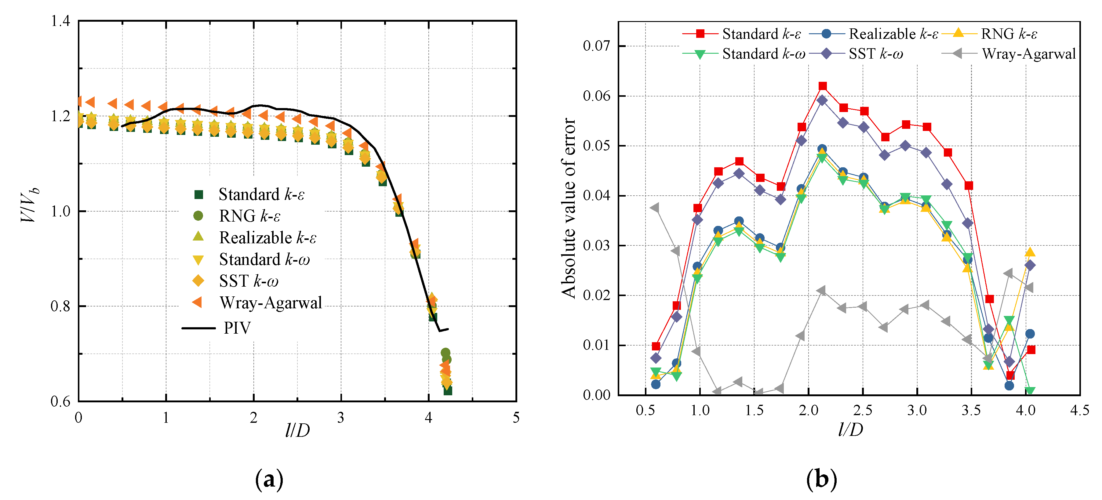
2.4. Turbulence Model Validation

In the numerical simulation, different turbulence models have different conditions of applicability. The selection of a suitable turbulence model not only allows for better coordination of computational resources but also for higher computational accuracy.

For the selection of computational models, this paper proposes to compare Wray–Agarwal, Standard k-ε, RNG k-ε, Realizable k-ε, Standard k-ω, and SST k-ω. All the above turbulence models are widely used in related research in the field [30,31] and have good simulation effects on complex flows such as secondary flows and cyclonic flows. Among them, the Wray–Agarwal [32,33] model is a one-equation linear eddy viscosity model that was derived from two-equation k-ω closure. It combines the most desirable characteristics of the one-equation k-ε model and the one-equation k-ω model. It uses the ω equation with a cross-diffusion term to increase the ability to solve for nonequilibrium flows, aiming to improve the accuracy of predicting the equilibrium flows [34,35,36].

Eddy viscosity:

$${\mu }_{\tau }=f_{\mu }\rho R,$$

(4)

$$R=\frac{k}{\omega },$$

(5)

R transport equation:

$$\begin{array}{l}\frac{\partial \rho R}{\partial \mathrm{t}}+\frac{\partial \rho u_{j}R}{\partial x_j}=\frac{\partial }{\partial x_j}\left[\left({\sigma }_R{\mu }_{\tau }+\mu \right)\frac{\partial R}{\partial x_j}\right]+\rho C_{1}RS\\ +\rho f_1{C}_{2k\omega }\frac{R}{S}\frac{\partial R}{\partial x_j}\frac{\partial S}{\partial x_j}-\left(1-f_1\right)\rho C_{2k\epsilon }\left(\frac{R\frac{\partial S}{\partial x_j}}{S}\right)\end{array}$$

(6)

where f_μ is the damping function; f₁ is the switching function; k is the turbulent pulsation kinetic energy, J; ω is the specific dissipation rate; t is the time, s; S is the average strain, 1/s; and the modulation constants C₁, C_2kω, C_2kε, and σ_R are determined from empirical data and the wall constraint law:

$$\begin{gathered} C_{1\mathrm{k}\omega }=0.0829, C_{1k\epsilon }=0.1127, C_1=f_1\left(C_{1\mathrm{k}\omega }-C_{1k\epsilon }\right)+C_{1k\epsilon } \\ {\sigma }_{k\omega }=0.72, {\sigma }_{k\epsilon }=1.0, {\sigma }_R=f_1\left({\sigma }_{k\omega }-{\sigma }_{k\epsilon }\right)+{\sigma }_{k\epsilon } \\ {C}_{2\mathrm{k}\omega }=\frac{C_{1k\omega }}{{\kappa }^2}+{\sigma }_{k\omega }, C_{2\mathrm{k}\epsilon }=\frac{C_{1k\epsilon }}{{\kappa }^2}+{\sigma }_{k\epsilon }, \kappa =0.41 \end{gathered}$$

(7)

Average strain:

$$S=\sqrt{2S_{ij}{S}_{ij}},$$

(8)

The damping function f_μ is given by:

$$f_{\mu }=\frac{{\chi }^3}{{\chi }^3+C_W^3},$$

(9)

$$\chi =\frac{R}{v},$$

(10)

It is important to note that more detailed information and descriptions of the Wray–Agarwal turbulence model can be found on the NASA Turbulence Modeling Resource (TMR) website (https://turbmodels.larc.nasa.gov/wray_agarwal.html, accessed on 29 July 2022).

HSJs have better conditions for turbulence development. On the other hand, they lack fast-changing parameters, namely the velocity gradients to characterize the accuracy of turbulence models for flow prediction. Based on the group’s previous experimental study of PIV for oblique submerged impact jets [37], the distribution of axial dimensionless velocity V/V_b along the jet axis under fixed impact angle (θ = 45°) and impact height (H/D = 3) conditions are calculated using the above turbulence models as shown in Figure 5a. The predicted results of different turbulence models are in good agreement with each other in the prediction of the jet flow trend, i.e., the axial velocity remains basically constant in the free jet region (0 ≤ l/D ≤ 3) and decreases rapidly in the impact region (3 ≤ l/D ≤ 4). The absolute errors between the results from either numerical simulation or PIV experiments in the effective monitoring range are shown in Figure 5b. Combining Figure 5a with Figure 5b, in the initial stage of the free jet (0 ≤ l/D ≤ 0.8), the predicted results of conventional turbulence models such as SST k-ω show high accuracy, while the predicted results of the Wray–Agarwal model are up to 3.3 % larger. With the free development of the jet, both the simulation results and the PIV experimental data show a slightly increasing trend. The results from Wray–Agarwal turbulence model fit better with the measurement results. At the same time, it is noted that as the velocity gradient and pressure gradient at the near-wall surface increase, the numerical results derived from each turbulence model are less and less different from the experimental data, showing a better prediction accuracy. The differences between the predicted results of each turbulence model gradually decrease and all agree well with the experimental data. Overall, the predicted results of the Wray–Agarwal turbulence model are larger. Meanwhile, the Wray–Agarwal model fits well with the results from experiments in most of the regions. It is noteworthy that the predicted results deviate from those from experiments in the jet exit region where the l/D is small. The focus of this paper is on capturing and analyzing the flow field structure within the HSJ, rather than focusing on the microscopic flow in the inlet region of the jet. Therefore, the prediction error in the jet exit area is considered acceptable. Through the above consideration, this paper decided to use the Wray–Agarwal model for numerical simulation.

3. Results and Discussion

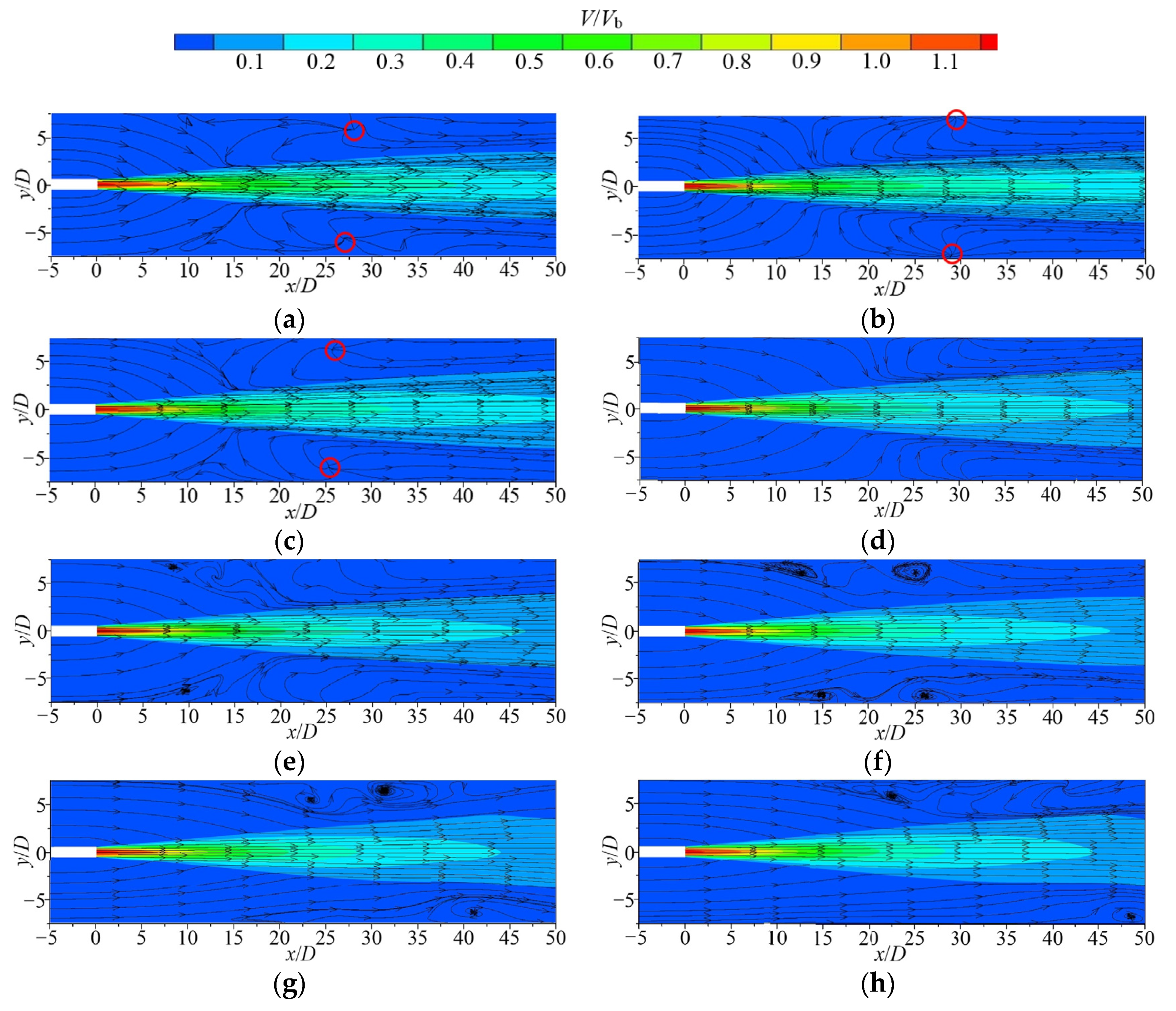
3.1. Flow Field Analysis

Figure 6 depicts the distributions of V/V_b with streamlines on the mid-section (oxz plane) of the jet at different horizontal heights (Re = 35,100). The parameter h is the vertical height from the bottom of the sink. As the surrounding fluid is continuously sucked into the jet, the jet gradually diffuses with decreasing axial velocity. When the horizontal height H/D equals 0.5, the HSJ structure is similar to a wall jet, where the jet diffusion near the wall side (along −z direction) is blocked. The jet diffuses freely away from the wall side (along +z direction). When the horizontal height is in the range of 0.5 < H/D ≤ 2, the jet spreads to the bottom wall in a relatively short time. As the H/D is larger than 2, the main stream of the jet moves towards the bottom wall. The mass on the side away from the wall is more than the side near the wall which is due to the unequal mass distribution of the ambient fluid affected by entrainment on both sides of the jet at the same time. With the turbulent mixing effect on the boundary of the jet, the energy transferred from the jet to the ambient fluid on both sides is basically equal. Hence, the entrainment velocity in the −z direction is larger, while the pressure is smaller, resulting in a shift of the main stream of the jet along the −z direction. The jet attachment effect then occurs. In addition, a vortex (E₁) appeared downstream of the jet exit. The vortex affected about 1/3 of the entire length of the flume. As the horizontal height of the jet increases, the position of the vortex core at the outlet gradually moves along the +z direction and the area of influence becomes smaller (E₅–E₇) until it disappears. This suggests that the associated backflow is more likely to occur in areas outside the main stream diffusion zone of the jet. The back flow needs some space for further development. At the same time, when H/D is small, the distributions of the entrainment area and the scope of the vortex in the flow field are highly consistent. The vortex areas (E₁–E₆) are both located in the upper right of the calculation domain and the boundary between them is clear and located near x/D = 30. Due to the entrainment effect, the jet will absorb a large amount of ambient fluid into the main stream. With a smaller H/D, there is not enough space for entrainment below the jet, resulting in a large amount of fluid being sucked into the area above the jet. With the full development of the jet, the fluid in the upper part of the computational domain at x/D = 30 reaches a certain entrainment velocity in the −z direction and mixes with the ambient fluid, forming a large reflux zone. As the H/D increases, the volume of entrainment on both sides of the jet gradually becomes equal. Meanwhile, the unsteady flow is relatively smaller, and the flow field in the sink is more regular.

Figure 7 shows the contours of the V/V_b velocity distribution with streamlines on the jet cross section (oxy plane) at different horizontal heights (Re = 35,100). As for 0.5 ≤ H/D ≤ 1.5, both the velocity contours and diagrams of streamlines show good symmetries; no obvious vortexes appear in the flow field. All of them have vector rotation points (VRP) which are distributed within the parameter range of 25 ≤ x/D ≤ 30. They also show high symmetry, which is highlighted in the figure with a red circle. The explanation appears to be that when H/D is small, the jet is fully developed in the oxy plane. In the −z direction of the oxz plane, however, the development of the jet is inhibited by the bottom wall. Hence, the turbulent kinetic energy contained in the jet cannot be adequately exchanged with the ambient fluid in the oxy plane, such that there is not enough energy in the direction perpendicular to the main stream velocity to engage in entrainment action with the surrounding fluid. Only VRPs without intact vortex structures appear. At H/D = 2, the suppression effect of the bottom wall of the jet becomes weak. The vortexes begin to appear in the flow field of the jet and are symmetrically distributed on both sides of its main stream of the jet near the wall. With the increase in H/D, the vortex near the side wall continues to develop and gradually moves in the −x direction. The inhibitory effect of the wall on jet development basically disappears at larger H/D when the turbulence is fully developed and the high-speed zone of the jet is significantly reduced. At the same time, the momentum exchange phenomenon with the ambient fluid is significant. This results in a significant increase in unstable three-dimensional flow in the flow field, creating an asymmetric distribution of the cross-sectional flow field in the jet. More unsteady flow is observed on the main stream side of the jet and a relatively flat flow on the other side.

To understand the process of vortex generation and its development in the sink, the contours of V/V_b and streamlines for different vertical cross sections (oxz plane) at different horizontal heights (Re = 35,100) are compared and analyzed, as shown in Figure 8. Comparing Figure 7c with Figure 8a, it is not difficult to find that the formation of VRP originates precisely from the sinking of the fluid at the edges of the vortex caused by the spatial vortex structure consisting of E_1-0 to E_1-6. When H/D is 1, a vortex with a large influence range (E_1-0) appears downstream of the jet outlet in the middle section. The scope of the vortex gradually decreases (E_1-0~E_1-6) during the development of this vortex to both sides. A vortex (G_1-4) occurs near the bottom of the cross-section at y/D = 4. On the cross-section at y/D = 6, the core position of this vortex was almost unchanged. The vortex developed significantly, and the influence range gradually increased. At H/D = 3 and the same value of y, the scope of vortexes generated at the jet downstream outlet (E_3-0 and E_3-2) are smaller than those (E_1-0 and E_1-2) generated in H/D = 1. The reduction in space above the jet and the increase in the volume of entrainment below contribute to this phenomenon. The position of the vortex core moves along the +z direction as well. Meanwhile, the vortexes G_3-4 and G_3-6 move gradually in the +x direction. Therefore, the incidence height H/D affects the size and location of the vortex in the flow field. There are obvious wall vortexes that are generated and well developed on both sides along the y-direction.

With different longitudinal sections x/D, the contour of V/V_b on the longitudinal section of the jet (oyz plane) at different horizontal heights at Re = 35,100 is depicted in Figure 9. The values of V/V_b for each longitudinal section of the jet are distributed in a circular pattern for different H/D conditions. The dimensionless velocity decreases gradually from the jet center to the edge. The entrainment effect during the development of the jet makes the jet flow increase along the range; the section is expanding, and the velocity gradually decreases. At H/D = 0.5, the jet flows along the bottom wall and diffuses more obviously along the lateral direction y than in the vertical direction z, indicating that the bottom wall limits the diffusion of the jet in the vertical direction and enhances the lateral diffusion. As H/D increases, the influence of the bottom wall on the jet becomes weak. At the same time, the velocity of the jet arriving at the cross-section of x/D = 50 becomes smaller with the increase in H/D. The relative high-speed region in the center of the V/V_b distribution contours gradually disappears. Indicating that with the increase in H/D, the energy exchange between the jet and the ambient fluid becomes more adequate, leading to the rapid dissipation of its own energy.

Figure 10 shows the variations of V/V_b at different horizontal heights at Re = 35,100. The cyan dashed line with arrows in the figure indicates the variation of the position of the maximum axial velocity point in the z-direction. As shown in the figure, the jet gradually spreads, and the maximum axial velocity gradually decreases as the jet flow x increases at H/D = 0.5. Due to the influence of the bottom wall, the parameter V/V_b distributes asymmetrically. The values of V/V_b near the bottom wall increase rapidly from 0 to the maximum. On the side of the HSJ away from the bottom, the values of V/V_b distribution are similar to the free jet velocity distribution. As the jet flow x increases, the point where V/V_b reaches the maximum value is gradually deviated from the central axis of the jet (x-axis) and gradually approaches the bottom wall. At H/D = 1, the maximum value of V/V_b is obtained on the centerline at x/D = 10. As for H/D = 0.75, however, the maximum value of V/V_b at the same position has deviated from the axis. This indicates that the distance between the position where the deflection of the jet occurs and the jet outlet increases with the growth of the horizontal height. As for H/D = 6, the bottom wall has almost no effect on the velocity distributions of the cross-section in the jet. The velocity distribution at each section is almost symmetric to the axis line. In summary, the bottom wall restricts the diffusion of the horizontal jet in the −z direction, increasing the axial velocity of the jet in the near-wall area. It then forms a low-pressure area below the main stream of the jet, which makes the jet deflect downward and leads to the wall attachment effect of the jet.

Figure 11 shows the distribution of V/V_b along the axis of the horizontal jet at different horizontal heights (Re = 35,100). The trends are similar at different horizontal heights. In the initial range (0 ≤ x/D ≤ 6), the values of V/V_b decrease slowly from 1.23 to 1.15. When the jet further develops, it decays rapidly to about 0.4 in the region of 6 ≤ x/D ≤ 25. As x/D continues to increase, the rate of decrease in V/V_b slows down and gradually fluctuates around 0.2. At the same time, due to the influence of the bottom wall, the mixing effect with the ambient fluid below the jet is greatly weakened. This is why the values of V/V_b of the horizontal jet with H/D = 0.5 are up to 1.29 times larger than those of other horizontal heights in the region of x/D > 6.

The distributions of each axial velocity have obvious inflection points. The horizontal inundation jet is divided into two zones. In zone I, the velocity drops sharply. In zone II, the drop of axial velocity slows down. To explore the general law of the inflection point, its first-order derivative image is made, as shown in Figure 12. The minimal value points of the V/V_b distribution curves under different H/D conditions are more concentrated and are all located near x/D = 10, suggesting that the inflection points of each axial velocity distribution curve have high consistency. The initial velocity of the jet is very fast after it is ejected from the outlet and mixed with the ambient fluid. During the process, there is a strong energy exchange and the axial velocity decreases along the course. As mentioned above, the cross-sectional area increases while the jet flow increases along the range, due to the entrainment effect, which leads to increased resistance of the main stream of the jet during its development, thus leading to an increase in the decay rate of the jet axial velocity and reaching a maximum at x/D = 10. As for x/D > 10, the jet gradually develops completely, and the energy exchange and entrainment effect then reach a relative equilibrium. The axial velocity decay rate remains at a low level and decreases along the range, which leads to an obvious inflection point on the V/V_b distribution curve. Further exploration reveals that although the extreme points (inflection points) of the first-order derivative images of each curve are consistent, there are large differences in their distributions of extreme value. When the horizontal height H/D is taken as 0.5 and 1.5, respectively, the extreme values of the corresponding axial velocity distribution curves obtain the maximum or minimum values. This indicates that at H/D = 0.5 and 1.5, the absolute value of the jet axial velocity gradient at the inflection point (x/D = 10) achieves the minimum and maximum values, respectively, due to the wall effect generated at the bottom wall. With the full development of the jet, a situation diametrically opposite to that described earlier emerges: the absolute value of the velocity gradient of V/V_b is maximum when the horizontal height H/D = 0.5, and the absolute value of the velocity gradient of V/V_b is minimum when the horizontal height H/D = 1.5.

Figure 13 shows the variations of V/V_b at different oxy and oxz cross-sections at different horizontal heights (Re = 35,100). At H/D = 0.5, z/D = ±0.25 and y/D = 0.25, the values of V/V_b almost remain as a constant in the range of 0 ≤ x/D ≤ 2. The values of V/V_b for each operating condition decrease gradually with the increase in the jet flow distance. The values of V/V_b in the range of 2 ≤ x/D ≤ 40 is located at z/D = −0.25, y/D = 0.25, and z/D = 0.25 cross-sections from the largest to the smallest. This indicates that the velocity of the jet fluid on the side close to the wall is increased due to the influence of the wall. The values of V/V_b at z/D = 0.5 and y/D = 0.5 rapidly increase from 0 to 0.6 in the region of 0 ≤ x/D ≤ 2. Meanwhile, the values of V/V_b at z/D = 0.5 and y/D = 0.5 gradually decrease. For H/D ≥ 2, the values of V/V_b at z/D = ±0.25 and y/D = 0.25 are almost equal, and the trend of velocity distribution is the same. Combined with Figure 8, the overall dimensionless velocity V/V_b of the jet is less and less influenced by the wall as H/D increases. In summary, the influence of the bottom wall on the jet is mainly manifested by limiting the diffusion in the −z direction, increasing the velocity in the near-wall area, and the influence of the bottom wall on the jet decreases with the increase in the horizontal height until it disappears.

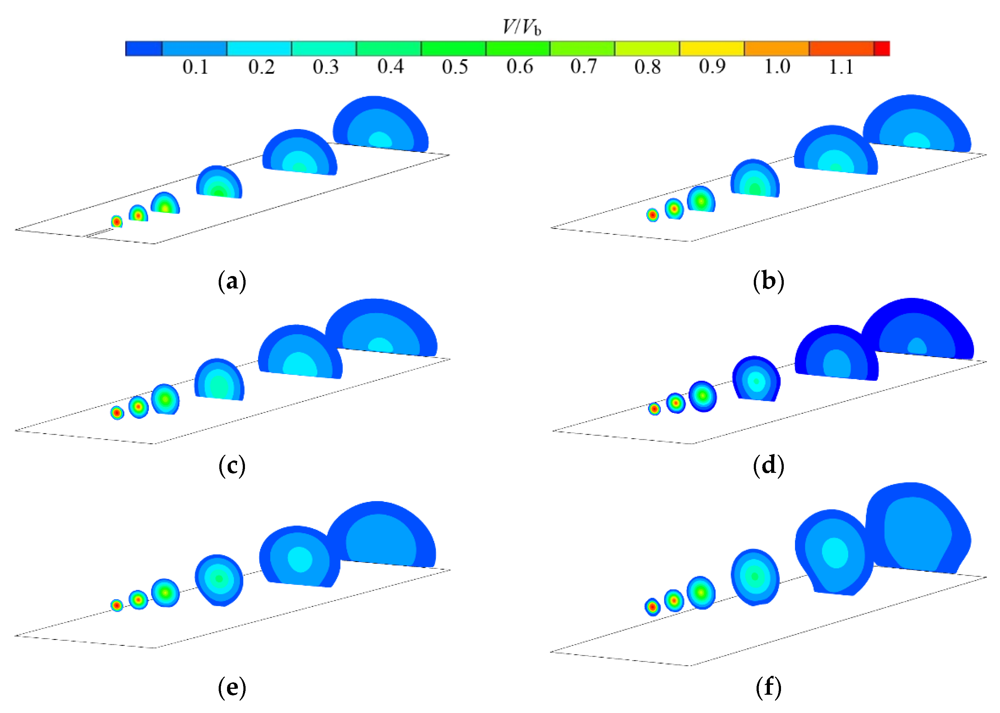
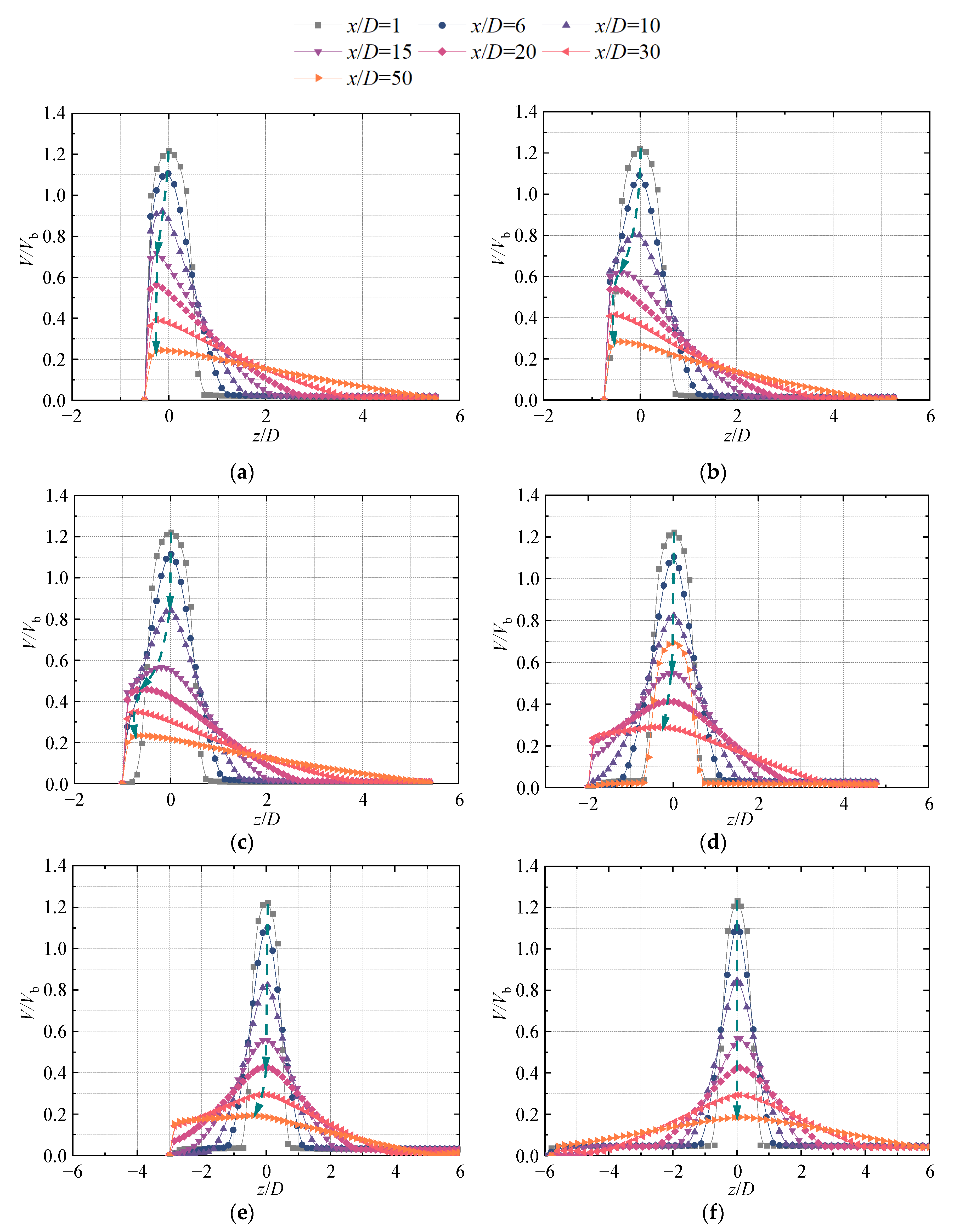
3.2. Jet Velocity Distribution in the Near-Wall Region

Figure 14 shows the contours of dimensionless velocity with the surface streamlines in the mid-section of the horizontal jet under the condition of horizontal height 0.5 ≤ H/D ≤ 1.5 in the parameter ranges of 0 ≤ x/D ≤ 10 and 0 ≤ H/D ≤ 2. The red rectangular block indicates the point where the pressure on the bottom wall is zero and is called the jet contact point (JCP). The JCP parameter gradually moves downstream of the jet with the increase in H/D. At H/D = 0.5, the jet flows along the bottom wall. At H/D = 0.75, the jet diffuses to the bottom wall at the position around x/D = 1.5, after which, the bottom wall restricts the vertical downward diffusion of the jet, resulting in a continuous backward movement of the JCP. On the side away from the bottom, however, the diffusion of the jet upward is almost unaffected, which leads to an asymmetry in the jet velocity distribution and vector diagram.

In order to explore the general law of JCP distribution, the horizontal distance of the JCP from the jet pipe outlet is denoted by L_p. Figure 15 depicts the variation of the L_p/D with H/D for different Reynolds number conditions. As shown in the figure, at a lower Reynolds number, the jet contains less turbulent kinetic energy and its ability to mix the ambient fluid is diminished, resulting in a small L_p/D in most of the H/D range. In particular, in the smaller H/D case (H/D = 0.75), the wall attachment effect of the HSJ is very weak because there is very little ambient fluid below the main stream of the jet. At the same time, the lower jet velocity further weakens the wall attachment effect, and the main stream of the jet is no longer deflected towards the bottom wall. In addition, the fluid below the main stream of the jet has a large velocity gradient in the z-direction, which produces a clear boundary layer effect. The slip phenomenon occurs when the jet main stream diffuses to the boundary layer, resulting in a large L_p/D for a small H/D. Overall, the distribution pattern of L_p/D under different Reynolds number conditions has a high consistency and shows a relatively independent property from the Reynolds number when the Reynolds number of the jet increases.

Figure 16 depicts the distribution of V/V_b at different values of z in the near-wall region in the parameter range of 0 ≤ z/D ≤ 0.5. When H/D = 0.5, the jet structure is a typical wall jet. The values of V/V_b decrease gradually with the increase in the jet range. At H/D = 0.75, the distribution of V/V_b shows different trends for different z values. At h/D = 0.1 and 0.2, the values of V/V_b increase gradually as x increases in the region of 0 ≤ x/D ≤ 10 due to the entrainment effect of the jet, and thereafter, the values of V/V_b decrease gradually. The velocity gradient when the jet decelerates is smaller than that when the flow is accelerated. As for increasing h/D, the values of V/V_b decrease gradually with the increase in the jet range, and is especially noted that when h/D = 0.3; a velocity smoothing zone appears near the outlet by the influence of the boundary layer of the main stream of the jet. In the zone, the values of V/V_b fluctuate around 0.72. When the H/D ranges from1.25 to 2, the velocity in the near-wall area shows a trend of gradual acceleration from 0. After that, a slow deceleration can be found. At the same time, V/V_b gradually approaches 0.2 as the horizontal height increases. In addition, the acceleration zone near the wall gradually expands.

4. Conclusions

In this paper, based on the Wray–Agarwal turbulence model, a numerical simulation study of HSJs with different incidence heights is carried out, and the main conclusions are as follows:

(1)

The jet horizontal height H/D has a large effect on the flow field structure of HSJ. When H/D is small, the unsteady structure in the jet flow field is dominated by vortexes, and the distribution is more regular, all starting generation around x/D = 30. In the meantime, the vortex structure in the flow field has a clear boundary and is insensitive to the variation of H/D. In addition, significant wall-attached vortexes are generated on both sides of the flow field. In the +y direction, the wall-attached vortexes gradually develop. They are also observed to gradually move in the +x direction as H/D increases.

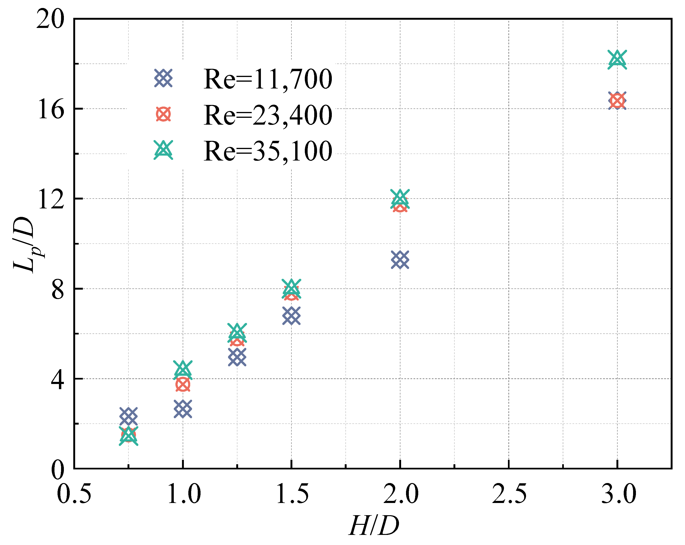
(2)

The distance between the JCP and the jet pipe outlet increases linearly with the increase in the incidence height H/D, but the distribution pattern of the JCP gradually becomes relatively independent of the Reynolds number with the increase in the jet Reynolds number.

(3)

The velocity distribution of the jet axial velocity under different incidence heights H/D has very high similarity, and all of them have obvious velocity inflection points at x = 10D. The horizontal inundation jet is divided into two zones; in zone I, the velocity drops sharply, while in zone II, the drop of axial velocity slows down. In addition, when H/D is small, its axial speed is significantly higher than in other working conditions, up to 1.29 times. It can be seen that the wall attachment effect of the jet and the boundary layer effect generated at the bottom of the fluid domain have a certain role in maintaining the velocity of the jet near the wall. The flow velocity of the main stream of the jet near the wall is obviously large. This phenomenon disappears with the increase in H/D. In addition, this velocity retention effect is most significant at H/D = 1.

The above conclusions have a certain guiding significance for engineering practice. In marine engineering, horizontal inundation jets are often used for underwater sand flushing and dredging where the distribution law of the horizontal jet JCP can be fully utilized, and the position of the JCP can be adjusted by controlling the incidence height to achieve precise construction. At the same time, the incidence height can be sufficiently reduced to ensure a large axial velocity of the jet in order to achieve a better scouring effect. It is not negligible that the vortex structure in the flow field is fully developed and has a stable distribution pattern at a small incidence height, which also provides good conditions for the rapid transport of scouring materials. In addition, in water conservancy engineering, horizontal submerged jet energy dissipation as a new flood energy dissipation method is developing rapidly, and the research results of this paper lay the theoretical foundation for the study of its energy dissipation effect, which is of great practical significance.

References

1. Dong, Z. Impinging Jets; China Ocean Press: Beijing, China, 1997. [Google Scholar]
2. Rouse, H. Cavitation in the mixing zone of a submerged jet. La Houille Blanche 1953, 1, 9–19. [Google Scholar] [CrossRef]
3. Law, H.S. Numerical prediction of the flow field due to a confined laminar two-dimensional submerged jet. Comput. Fluids 1984, 12, 199–215. [Google Scholar] [CrossRef]
4. Wen, Q.; Kim, H.D.; Liu, Y.; Kim, K.C. Dynamic structures of a submerged jet interacting with a free surface. Exp. Therm. Fluid Sci. 2014, 57, 396–406. [Google Scholar] [CrossRef]
5. Liu, H.; Kang, C.; Zhang, W.; Zhang, T. Flow structures and cavitation in submerged waterjet at high jet pressure. Exp. Therm. Fluid Sci. 2017, 88, 504–512. [Google Scholar] [CrossRef]
6. Yang, Y.; Li, W.; Shi, W.; Zhang, W.; El-Emam, A.M. Numerical Investigation of a High-Pressure Submerged Jet Using a Cavitation Model Considering Effects of Shear Stress. Processes 2019, 7, 541. [Google Scholar] [CrossRef]
7. Ma, J.; Song, Y.; Zhou, P.; Cheng, W.; Chu, S. A mathematical approach to submerged horizontal buoyant jet trajectory and a criterion for jet flow patterns. Exp. Therm. Fluid Sci. 2018, 92, 409–419. [Google Scholar] [CrossRef]
8. Yang, H.C. Horizontal two-phase jet behavior with an annular nozzle ejector in the water tank. J. Vis. 2015, 18, 359–367. [Google Scholar] [CrossRef]
9. Xi, B.; Wang, C.; Xi, W.; Liu, Y.; Wang, H.; Yang, Y. Experimental investigation on the water hammer characteristic of stalling fluid in eccentric casing-tubing annulus. Energy 2022, 253, 124113. [Google Scholar] [CrossRef]
10. Shao, D.; Huang, D.; Jiang, B.; Law, A.W.K. Flow patterns and mixing characteristics of horizontal buoyant jets at low and moderate Reynolds numbers. Int. J. Heat Mass Transf. 2017, 105, 831–846. [Google Scholar] [CrossRef]
11. Chatterjee, S.S.; Ghosh, S.N.; Chatterjee, M. Local scour due to submerged horizontal jet. J. Hydraul. Eng. 1994, 120, 973–992. [Google Scholar] [CrossRef]
12. Chiew, Y.M.; Lim, S.Y. Local scour by a deeply submerged horizontal circular jet. J. Hydraul. Eng. 1996, 122, 529–532. [Google Scholar] [CrossRef]
13. Tang, S.; Zhu, Y.; Yuan, S. Intelligent Fault Diagnosis of Hydraulic Piston Pump Based on Deep Learning and Bayesian Optimization. ISA Trans. 2022, in press. [Google Scholar] [CrossRef]
14. Zhu, Y.; Li, G.; Tang, S.; Wang, R.; Su, H.; Wang, C. Acoustic Signal-based Fault Detection of Hydraulic Piston Pump using a Particle Swarm Optimization Enhancement CNN. Appl. Acoust. 2022, 192, 108718. [Google Scholar] [CrossRef]
15. Abdelaziz, S.; Bui, M.D.; Rutschmann, P. Numerical simulation of scour development due to submerged horizontal jet. River Flow 2010, 2010, 1597–1604. [Google Scholar]
16. Li, H.; Zheng, T.; Dai, L.; Chen, X. Theoretical Research on New Energy Dissipation Type of Multi-horizontal Submerged Jets. Water Resour. Power 2010, 20, 74–76+166. [Google Scholar]
17. Li, W.; Zhang, W.; Shi, W.; Yang, Y.; Cao, W. Experiment study on cavitation cloud evolution law of cavitation jet of convergent-divergent nozzle. J. Irrig. Drain. Eng. 2020, 38, 547–552. [Google Scholar]
18. Kan, B.; Gao, Y.; Xu, S.; Ding, J. Numerical simulation of flow field characteristics of pressure controllable pipe with microporous walls. J. Irrig. Drain. Eng. 2020, 38, 183–187. [Google Scholar]
19. Qi, M.; Wang, L.; Chen, Q.; Zhao, J.; Ju, Y.; Fu, Q. Numerical simulation of cavitating jet in dual chamber self-oscillation pulse nozzle. J. Irrig. Drain. Eng. 2020, 38, 457–461. [Google Scholar]
20. Jiang, H.; Yan, H.; Xiao, Z.; Cheng, L.; Liu, H. Numerical simulation of hydraulic characteristics of three-side inlet of vertical shaft inlet channel of horizontal pumping station. J. Irrig. Drain. Eng. 2021, 39, 1008–1013. [Google Scholar]
21. Shi, G.; Yao, X.; Wang, S.; Li, H. Analysis of stress and strain of multiphase pump blade considering medium viscosity. J. Irrig. Drain. Eng. 2020, 38, 991–996. [Google Scholar]
22. Zhang, H.; Zheng, Y.; Zhang, Z.; Kan, K.; Mo, X. Influence of placement angle of sewage mixer on its hydraulic characteristics. J. Irrig. Drain. Eng. 2021, 39, 483–487. [Google Scholar]
23. Wang, H.; Long, B.; Wang, C.; Han, C.; Li, L. Effects of the impeller blade with a slot structure on the centrifugal pump performance. Energies 2020, 13, 1628. [Google Scholar] [CrossRef]
24. Liu, Y.; Pan, Z. Analysis of internal flow characteristics of marine water-jet propulsion. J. Irrig. Drain. Eng. 2022, 40, 55–61. [Google Scholar]
25. Quan, H.; Cheng, J.; Peng, G. Effect of screw centrifugal inducer on mechanical characteristics of vortex pump. Drain. Irrig. Mach. Eng. 2021, 39, 345–350. [Google Scholar]
26. Roache, P.J. A method for uniform reporting of grid refinement studies. ASME-Publ.-Fed 1993, 158, 109. [Google Scholar] [CrossRef]
27. Khayrullina, A.; van Hooff, T.; Blocken, B.; van Heijst, G. Validation of steady RANS modelling of isothermal plane turbulent impinging jets at moderate Reynolds numbers. Eur. J. Mech. B/Fluids 2019, 75, 228–243. [Google Scholar] [CrossRef]
28. Liu, H.; Liu, M.; Bai, Y.; Du, H.; Dong, L. Grid convergence based on GCI for centrifugal pump. J. Jiangsu Univ. Nat. Sci. Ed. 2014, 35, 279–283. [Google Scholar]
29. Celik, I.B.; Ghia, U.; Roache, P.J.; Freitas, C.J. Procedure for estimation and reporting of uncertainty due to discretization in CFD applications. J. Fluids Eng. Trans. ASME 2008, 130, 7. [Google Scholar]
30. Ying, J.; Yu, X.; He, W.; Zhang, J. Volume of fluid model-based flow pattern in forebay of pump station and combined rectification scheme. J. Irrig. Drain. Eng. 2020, 38, 476–480. [Google Scholar]
31. Feng, L.; Xu, R.; Feng, J. Numerical simulation of flow and heat transfer characteristics in helical pipe. J. Irrig. Drain. Eng. 2020, 38, 697–701. [Google Scholar]
32. Wray, T.J.; Agarwal, R.K. Low-Reynolds-number one-equation turbulence model based on k-ω closure. AIAA J. 2015, 53, 2216–2227. [Google Scholar] [CrossRef]
33. Han, X.; Rahman, M.; Agarwal, R.K. Development and Application of Wall-Distance-Free Wray-Agarwal Turbulence Model (WA2018). In Proceedings of the 2018 AIAA Aerospace Sciences Meeting, Kissimmee, FL, USA, 8–12 January 2018; p. 0593. [Google Scholar]
34. Hu, B.; Wang, H.; Liu, J.; Zhu, Y.; Wang, C.; Ge, J.; Zhang, Y. A Numerical Study of a Submerged Water Jet Impinging on a Stationary Wall. J. Mar. Sci. Eng. 2022, 10, 228. [Google Scholar] [CrossRef]
35. Zhang, D.; Wang, H.; Liu, J.; Wang, C.; Ge, J.; Zhu, Y.; Chen, X.; Hu, B. Flow Characteristics of Oblique Submerged Impinging Jet at Various Impinging Heights. J. Mar. Sci. Eng. 2022, 10, 399. [Google Scholar] [CrossRef]
36. Xu, W.; Wang, C.; Zhang, L.; Ge, J.; Zhang, D.; Gao, Z. Numerical study of continuous jet impinging on a rotating wall based on Wray–Agarwal turbulence model. J. Braz. Soc. Mech. Sci. Eng. 2022, 44, 433. [Google Scholar] [CrossRef]
37. Wang, C.; Wang, X.; Shi, W.; Lu, W.; Tan, S.K.; Zhou, L. Experimental investigation on impingement of a submerged circular water jet at varying impinging angles and Reynolds numbers. Exp. Therm. Fluid Sci. 2017, 89, 189–198. [Google Scholar] [CrossRef]
Figure 1. Schematic diagram of the three-dimensional horizontal submerged jet.
Jmse 10 01217 g001
Figure 2. The distribution of the axial velocity V/Vb of the jet for the different numbers of grids.
Jmse 10 01217 g002
Figure 3. GCI distribution of numerical simulation results.
Jmse 10 01217 g003
Figure 4. Schematic diagram of the computational model grid.
Jmse 10 01217 g004
Figure 5. Results and analysis of V/Vb obtained from different turbulence models: (a) Distribution of axial velocity V/Vb along the axis of the jet; (b) Absolute error values of numerical results and PIV experiments.
Jmse 10 01217 g005
Figure 6. Contours with streamline diagrams of cross-sectional V/Vb distribution (oxz plane) in the jet under different H/D conditions: (a) H/D = 0.5; (b) H/D = 0.75; (c) H/D = 1; (d) H/D = 1.5; (e) H/D = 2; (f) H/D = 3; (g) H/D = 4; and (h) H/D = 6.
Jmse 10 01217 g006
Figure 7. Contours with streamline diagrams of V/Vb distribution in the jet cross-section (oxy plane) under different H/D conditions: (a) H/D = 0.5; (b) H/D = 0.75; (c) H/D = 1; (d) H/D = 1.5; (e) H/D = 2; (f) H/D = 3; (g) H/D = 4; and (h) H/D = 6.
Jmse 10 01217 g007
Figure 8. Contours with streamline diagrams of V/Vb distribution for different shot vertical sections: (a) H/D = 1; (b) H/D = 3.
Jmse 10 01217 g008
Figure 9. V/Vb distribution contours of longitudinal section (oyz plane) of jet under different H/D conditions: (a) H/D = 0.5; (b) H/D = 1; (c) H/D = 1.5; (d) H/D = 2; (e) H/D = 3; and (f) H/D = 4.
Jmse 10 01217 g009
Figure 10. Axial V/Vb distribution in the mid-section (oxz plane) of the jet under different H/D conditions: (a) H/D = 0.5; (b) H/D = 0.75; (c) H/D = 1; (d) H/D = 2; (e) H/D = 3; and (f) H/D = 6.
Jmse 10 01217 g010
Figure 11. Distribution of horizontal jet axial dimensionless velocity V/Vb at different horizontal heights.
Jmse 10 01217 g011
Figure 12. First-order derivative curve of V/Vb.
Jmse 10 01217 g012
Figure 13. Distribution of V/Vb at different y/D and z/D positions at different horizontal heights H/D: (a) H/D = 0.5; (b) H/D = 0.75; (c) H/D = 1; (d) H/D = 1.5; (e) H/D = 3; and (f) H/D = 4.
Jmse 10 01217 g013
Figure 14. Contours with vector diagrams of jet velocity distribution at different incidence heights H/D: (a) H/D = 0.5; (b) H/D = 0.75; (c) H/D = 1; (d) H/D = 1.25; and (e) H/D = 1.5.
Jmse 10 01217 g014
Figure 15. The plot of dimensionless distance Lp/D with H/D.
Jmse 10 01217 g015
Figure 16. Distribution of near-wall dimensionless velocity V/Vb at different incidence heights H/D: (a) H/D = 0.5; (b) H/D = 0.75; (c) H/D = 1; (d) H/D = 1.25; (e) H/D = 1.5; and (f) H/D = 2.
Jmse 10 01217 g016