Ensemble Neural Networks for the Development of Storm Surge Flood Modeling: A Comprehensive Review

Abstract

This review paper focuses on the use of ensemble neural networks (ENN) in the development of storm surge flood models. Storm surges are a major concern in coastal regions, and accurate flood modeling is essential for effective disaster management. Neural network (NN) ensembles have shown great potential in improving the accuracy and reliability of such models. This paper presents an overview of the latest research on the application of NNs in storm surge flood modeling and covers the principles and concepts of ENNs, various ensemble architectures, the main challenges associated with NN ensemble algorithms, and their potential benefits in improving flood forecasting accuracy. The main part of this paper pertains to the techniques used to combine a mixed set of predictions from multiple NN models. The combination of these models can lead to improved accuracy, robustness, and generalization performance compared to using a single model. However, generating neural network ensembles also requires careful consideration of the trade-offs between model diversity, model complexity, and computational resources. The ensemble must balance these factors to achieve the best performance. The insights presented in this review paper are particularly relevant for researchers and practitioners working in coastal regions where accurate storm surge flood modeling is critical.

1. Introduction

Rising sea levels increase the risk of coastal flooding depending on the relative rate of mean sea/land level changes [1,2,3]. The impacts are linked to concurrent near-term trends as well as gradual escalation of long-term coastal inundation risk over time [4]. Estuaries and coastal areas should adapt to changing climate and implement the necessary mitigation measures. A complex process such as a storm surge is sensitive to abrupt changes in several storm parameters, such as intensity, surface atmospheric pressure at the center of the storm, maximum sustained wind speed, size, and forward speed, in addition to the effects driven by the characteristics of dynamic coastal settings, such as shoreline geography, estuaries, and bay barriers [5]. The interdependency of these different factors make it notoriously hard to predict the timing and intensity of the hydrodynamic response (e.g., water levels and currents) [6,7,8,9]. Parametric models conventionally incorporate historical or synthetic hurricanes using storm size, intensity, and track, allowing for the prediction of storm surge heights and overland flooding [10,11].

During a storm surge event (caused by tropical or extratropical cyclones), the potential impacts extend beyond the surge itself and could exacerbate flooding and structural damage. This can be further intensified by the surface gravity waves due to the superimposed storm tide [12]. Wave driven set-ups can contribute up to $30\%$ of the total increase in water level (including both typical fluctuations and any additional rise) along the coast [13]. The combination of elevated water levels along with the destructive power of waves poses a tremendous danger to densely populated areas adjacent to coastal waters. The U.S. Atlantic and Gulf Coasts, for example, are expected to experience a sea level rise of, on average, 0.25–0.30 m in 30 years (2020–2050) [14]. This further increases the vulnerability of coastal regions to compound flooding (CF), where the interaction of rainfall, rivers, and ocean storm surges combine and create a cataclysmic force [15]. To overcome these challenges, physics-based approaches, such as hydrodynamic models, have been used to estimate hydrological processes and flood hazards/the probability of particular events that require land–atmosphere–ocean coupling [16]. Although these models explain the nature of flooding phenomena and show great skill for a wide variety of flood prediction scenarios, they usually deal with the physical dynamics and require various types of datasets, as the occurrence of floods varies with time and space [17,18]. This requires a large amount of computation, which makes short-term predictions very challenging. The reader is kindly referred to [17,19,20] for the comprehensive studies related to the development of physics-based models, their challenges, and capabilities.

Hydrodynamic modeling has also been extensively used to investigate the spatial and temporal variability of storm surges. Hydrodynamic models are widely utilized to describe coastal ocean processes and near-shore circulation and to simulate future scenarios of possible storm surge flooding [21]. These models are well-developed to account for the inherent uncertainties associated with sea level rise and storm surges. They also consider the relative impacts of different meteorological forces in total water levels [22,23]. However, these models are computationally demanding and time consuming. This limits their ability to simulate large complex domains or ensembles of events.

Some parametric models, such as the Bayesian model averaging, autoregressive integrated moving average, and peak over threshold methods, are among the most preferred methods to predict the statistical behavior of storm surge flooding [24,25]. However, these models are, at times, computationally demanding and typically sophisticated. Furthermore, generalizing the potential impacts of a storm surge for a particular geographical area to other areas with different parameters and settings is not a reliable approach [23]. Flood prediction requires constructing a minimum of a decade of non-tidal residual data from measurement by sea-level gauges [26]. In small datasets, i.e., those with a lack of large-sample observational data, even a few outliers will significantly alter the model or affect the correlation among the predicting variables [27].

Low-fidelity numerical storm surge models such as SLOSH (Sea, Lake, and Overland Surges from Hurricane) [28] are used by emergency managers and researchers to assist in forecasting the hydrodynamic response to a predicted hurricane track, size, and intensity. These models have significant uncertainty when used for forecasting [29,30]. Coupling ADCIRC (ADvanced CIRCulation model) [31] with WAM (WAve prediction Model) [32], STWAVE (Steady-State Spectral Wave Model) [33], or SWAN (Simulating WAves Nearshore) [34] is a widely used method for generating high-resolution storm surge models of specific regions [35,36]. Considering their additional wave forcing processes, finer mesh sizes, and smaller time steps, high-fidelity models are computationally more expensive [37]; thus, the accurate and quick assessment of hurricane-induced flooding has always been a challenging task.

Surrogate models are another approach to overcome this huge obstacle by simplifying approximations of more complex, higher-order models [10]. The Surge and Wave Island Modeling Study (SWIMS) [38] in the USACE, for example, developed a fast surrogate model by simulating hundreds of hurricanes to predict peak storm surges and hurricane responses in only a couple of seconds, which is an advantage over high-fidelity coupled simulations. Considering this issue, in a national-scale effort, the U.S. Army Engineer Research and Development Center developed a statistical analysis and probabilistic modeling tool named the StormSim Coastal Hazards Rapid Prediction System (StormSim-CHRPS) [39]. The tool preserves the accuracy of the high-fidelity hydrodynamic numerical simulation methods, such as ADCIRC, while significantly reducing computational demands, making it more convenient for real-time emergency management applications. The intricate input/output relationships inherent in high-fidelity numerical models are approximated using a machine learning method called Gaussian process metamodeling (GPM), enabling the rapid prediction of the peak storm surge and hurricane responses within seconds and for different hurricane scenarios.

Lee et al. [37] sought to enhance coastal resilience by providing a rapid storm surge prediction surrogate model called C1PKNet, a combination of a convolutional neural network model (CNN), principal component analysis, and a k-means clustering method, which was trained efficiently on a dataset of 1031 high-fidelity storm surge simulations. The resulting model is capable of predicting peak storm surges from realistic tropical cyclone track time series. A few studies, such as [40,41], even consider global warming, earth–moon–sun gravitational attractions, and storm surges to estimate the coastal sea level at an hourly temporal scale. The model in [40] was developed using an artificial neural network (ANN) approach called long short-term memory (LSTM) and trained on the ECMWF (European Center for Medium-Range Weather Forecasts) reanalysis dataset, ERA5 (more information on raw input data generation using ERA5 is available in Section 5.1).

To the best of our knowledge, only a limited number of researchers, such as [37,42,43,44] aimed to assess the concept of ANN ensemble learning for storm surge prediction. Braakmann-Folgmann et al. [43], for example, developed a combined convolutional and recurrent neural network to analyze both the spatial and the temporal evolution of sea level anomalies in the northern and central Pacific Ocean. They show how neural network architectures outperform simple regression to improve predictions for the future sea level. A novel deep learning architecture was implemented by [44] in contrast to a primitive model called the general ocean circulation model ensemble or NEMO (Nucleus for European Modelling of the Ocean). Their aim was to reduce the uncertainty associated with accurate sea level predictions and also to show the importance of sea level and atmospheric inputs for shorter forecast times. In the latter study, the ensemble ANN method for sea level forecasting known as HIDRA (HIgh-performance Deep tidal Residual estimation method using Atmospheric data) implements variants of temporal convolutional networks (TCN) and LSTM to encode temporal features of atmospheric and sea-level data. The dataset was trained on a 10-year (2006–2016) time series of atmospheric surface fields using a single member of the ECMWF atmospheric ensemble.

More recent papers such as [42,43] investigated the capability of different combinations of neural network (NN) models to predict surge levels. The fundamental core of this research revolves around selecting the best NN architecture for an ensemble approach to outperform a simple probabilistic model. Tiggeloven et al. [43], for example, combined a CNN-LSTM (ConvLSTM) model to capture the spatio-temporal dependencies for peak water level observations. This research has important implications for the sensitivity analysis of predictor variables and investigates how uncertainty in the predictions changes with input or architecture complexity. Tropical cyclones can also be parametrically represented via the joint probabilities method (JPM) [45]. However, the parametric description of complex systems, such as large-scale, non-frontal, low-pressure tropical cyclones, is intrinsically difficult to determine. As an alternative approach to these models, data-driven methods such as multiple linear regression [26,46], decision tree, ANN [40,42,43,47,48,49,50], and support vector machine [51,52] have been widely used for the prediction of storm surge heights. In most of studies where data-driven surrogate models are trained with physics-based simulations, such as ADCIRC [37,42,52], a major hurdle is the lack of sufficiently long datasets for training, validating and testing the surrogate models. As [53] explains, a long record in a storm surge reconstruction dataset is critical to capture as many storm events as possible; thus low-probability, high-impact, extreme events could be accounted for.

This review paper is structured as follows. Section 2 highlights the general concept of neural network ensembles and introduces several challenges and limitations. A theoretical framework for the geometry of neural networks, transfer learning, and their application to storm surge prediction models and different ensemble generation methods (i.e., how to combine the predictions from multiple models) are presented in Section 3. Section 4 discusses the less-debated topic of ensemble pruning and fine-tuning, the next stage after ensemble generation. Section 5 introduces data preparation considerations on developing an ensemble of neural networks, and different sources of datasets commonly used to predict storm surge levels are presented as well. Section 6 discusses some important factors and parameters regarding the best model selection and how the performance of the selected ensemble is evaluated. Finally, in Section 7, a summary is presented.

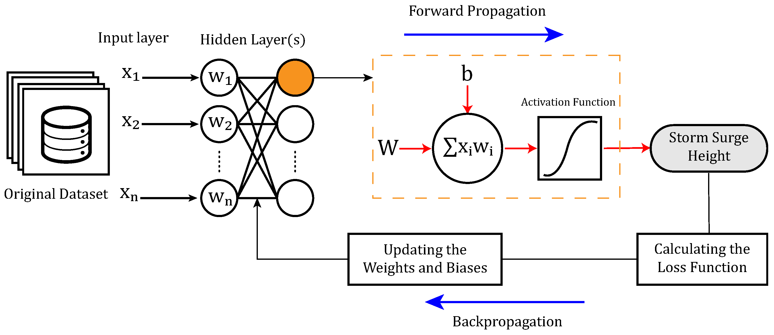
2. Neural Network Ensemble

Ensemble learning refers to techniques that involve combining the predictions of several base estimators based on classification or regression problems, aiming at improving predictability. This approach has gained a lot of attention in recent years, and the reported results regarding sea level rise projections have been satisfactory, such as in [7,44,54]. Ensembles have been reported to achieve higher certified robustness than single machine learning algorithms, as discussed in Section 2. Therefore, coastal hydrodynamic modeling techniques have been applied in ensemble with data-driven models such as deep learning techniques, especially neural networks, to develop ocean circulation and flood simulation models. This is due to the popularity and application of the finite element methods in numerical hydrodynamic models and their adequate modeling resolution [55,56,57]. These numerical models are conventionally applied to probabilistic coastal ocean forecast systems such as Surge Guidance System Forecasts (ASGS) or NOAA P-Surge to accommodate thousands of simulations [58].

Various types of neural networks are helpful to solve regression prediction problems where the aim is to predict the output of a continuous value such as water levels. Multilayer perceptrons (MLPs), a classical type of neural network, can reconstruct and validate atmospheric forcing, such as maximum sustained wind speed [59,60,61]. Convolutional neural networks (CNNs) have been developed to capture spatial and temporal dependencies for surge-level observations on a grid-based dataset and could potentially identify and predict regional and global patterns in storm and climate datasets [62]. They can also extract water bodies from remote sensing images [63]. Recurrent neural networks (RNNs) could be helpful in modeling storm behavior and time series of water levels in a sequence prediction framework [43], which requires a longer training time (not dependent on a fixed input size) compared to CNNs. Long short-term memory (LSTM), a subtype of RNN, is a successful model and has been used to capture long-term temporal dependencies of meteorological forcing [64,65] and to analyze the rapid intensification and occurrences of cyclones [66]. A diverse set of base learners (individual learners of the ensemble), such as MLPs, CNNs, and RNNs with appropriate training and tuning, is one empirical way to improve model performance by generating more complex models [67].

The focus of this paper is to introduce ensemble methods that can predict storm surge levels using a supervised ANN. Some challenges associated with using ANNs are the inability to capture peak water levels (due to the complex and nonlinear nature of the physical processes) [65,68], long-term processes (which are unavailable due to instrument failures, insufficient data, or sparse observational records), and predictions of storm surges at ungauged sites [43,69]. However, when utilized appropriately, ANN ensemble models have the potential to provide better and faster results than finite element hydrodynamic models. Figure 1 emphasizes the essential need for rapid prediction models, e.g., ENNs, by presenting a benchmark for the Aransas Wildlife Refuge station in Texas during and following Hurricane Harvey in 2017 [39]. This descriptive example compares storm surge predictions from a rapid empirical prediction model against water level observations from NOAA tide gauges and predictions from operational ADCIRC runs performed at the U.S. Army Engineer Research and Development Center’s Coastal and Hydraulics Laboratory (ERDC-CHL). Hurricane Harvey started as a modest tropical storm in August. However, after re-forming over the Bay of Campeche, it intensified rapidly into a category 4 hurricane. Harvey made its landfall along the central Texas coast and then stalled for four days, resulting in unprecedented rainfall, exceeding 1520 mm and resulting in a surge reaching 1.4 m across southeastern Texas [70]. Figure 1 also highlights the rate of change and meteorological and oceanographic observations during the hurricane. Forecasts are typically updated at 6 hour intervals. However, for unusual storm scenarios comparable to Hurricane Harvey with rapid approach trajectories or extended durations within flood plains, the expected update intervals can be reduced to 3 h or even shorter.

A thorough and extensive literature review can be found in [1,71], where machine learning models are compared to traditional physically based models.

3. Theoretical Framework

3.1. Neural Network Architectures

The NN architecture consists of individual members called neurons, which are combined to simulate the biological behavior of the brain to solve real-world problems [37,41]. Neural networks are not an exclusive standardized method; instead, they involve learning algorithms and architectures that can be applied to a wide range of supervised flood and storm surge forecasting models. These models use a set of individual independent variables, such as tidal and meteorological data points, and a real value dependent variable that represents the phenomenon, such as storm surge levels [42,43,72]. A general scheme is shown in Figure 2 based on a fully connected MLP representation. In the basic MLP architecture, the input layer is connected to one or multiple hidden layers and finally to the output layer to construct a fully connected system. The information is primarily processed in the forward direction (feed-forward) and is put through a linear transformation using a weights matrix [47,73]. An activation function defines how the weighted sum of the input vector is transformed to the neurons of the next layer [47]. The choice of activation function in both the hidden and output layers significantly influences the performance of the NN model in learning from the training dataset and predicting storm surge events. Empirical testing and cross-validation are essential to determine the most appropriate activation function that can effectively capture non-linear relationships within the data.

Table 1. Frequently used activation functions in ANN storm surge prediction models.

Activation Function	Equation	Python Library	Applications
ReLU (Rectified Linear Unit)	$f\left(x\right)=max(0,x)$	tensorflow, keras	MLP, CNN
Sigmoid	$f\left(x\right)=\frac{1}{1+e^{-x}}$	tensorflow, keras	RNN
Tanh (Hyperbolic Tangent)	$f\left(x\right)=\frac{e^x-e^{-x}}{e^x+e^{-x}}$	tensorflow, keras	RNN
Softmax	$f\left(x_j\right)=\frac{e^{x_j}}{{\sum }_{k=1}^K{e}^{x_k}}$	tensorflow, keras	Classification, normalizing the output
Leaky ReLU	$f\left(x\right)=max(\alpha x,x)$	tensorflow, keras	MLP, CNN

presents some frequently used activation functions specifically tailored for storm surge prediction models, as well as the relationship between each activation function and its corresponding Python library. The elementwise activation function is usually shifted with a bias to adjust the final output matrix. Different model configurations associated with learning processes and choices of the right dimensions of the NN structure, including the number of hidden layers, learning rate, batch size, choice of the activation function and loss function, etc., are referred to as hyperparameters [74,75,76].

Table 2. Classification of major hyperparameters in NN models.

Physical Components	Training/Optimization Procedures	Regularization
Number of hidden layers within the network	Defining the optimizer algorithm	Degree of regularization (lambda)
Number of hidden Neurons	Configuring the learning rate	Number of active neurons (dropout rate)
Choice of key activation function	Defining the main type of loss function
	Choice of evaluation metric for regression problem
	Number of training samples (mini-batch)
	Setting the random initialization
	Number of training cycles (epochs)

presents a summary of the major hyperparameters in NN models. These tuning parameters pertain to the physical components, training/optimization procedures, and regularization effect in a neural network.

In order to train a MLP feed-forward NN model, a backpropagation NN (BPNN) is widely used. This algorithm has been identified as one of the simplest and the most powerful ML prediction tools suitable for flood time series and short-term storm surge predictions [77,78,79,80]. In a BPNN algorithm, the gradient of the loss function (the vector of the partial derivatives) is calculated through a method called chain rule to adjust each weight and its contribution to the overall error. Further details of BPNN algorithms can be found in Appendix A.

3.2. Transfer Learning

In some scenarios, the NN algorithms use different sources of information such as historical tropical cyclones, topography, meteorological forcing, and other sources to make a complex network. Training an ensemble of NN models on such a massive volume of raw data can be computationally expensive [81]. On the other hand, when datasets are expensive or difficult to collect or data are scarce for a specific problem (such as the short-term analysis of hurricane tracks) [64,82], obtaining a training dataset to discern a meaningful pattern could be problematic. Transfer learning, as shown in Figure 3, is a functional method of tackling these problems through, i.e., building a high performance NN model while reducing training time [83]. This is performed by obtaining a high-accuracy and large pre-trained model from a related source and transferring the knowledge from the trained data to the target domain in a time-saving way [84]. Surge time series data over long time scales are usually subject to seasonal variability known as seasonality [85,86,87] (which can be simply defined using a Fourier transform and finding the seasonal frequencies). Removing seasonality from the time series data might happen during data preparation (which is further discussed in Section 5). Extractions of sparse time series samples from short-term extreme impacts during dominant seasons could be limited in size, implying that the insufficient training data are unable to represent the target efficiently [85]. Therefore, transferring knowledge from a diverse, large-scale, and pre-trained dataset of a time series of a similar task (with minor adjustments) could be reasonable [88] when a NN model is adapted to forecast a new time series, thus avoiding the need for additional training [83].

3.3. Ensemble Generation Methods

Ensemble neural networks basically consist of [54]: (1) generating multiple base learners (weak classifiers) and (2) combining the predictions to make a strong learner. The notion is that various classes of neural networks are created as base learners and then combined as a strong learner to predict the storm surge [55]. When ensemble members employ a single-type base learning algorithm but are generated upon a different subset of training data, they are classified as homogeneous [67,89]. Heterogeneous ensembles, on the other hand, consist of classifiers (base learners) of different types, such as MLP, CNN, or LSTM, which are usually trained on the same dataset [67,90]. These ensemble models are designed such that base learners are generated in sequential or parallel format. The basic motivation of the former is to create successive learning algorithms over iterations where predictions of a base learner are corrected and fine-tuned, then provided to the subsequent base learners. In the latter, the base learners are generated in parallel and independent from each other. Predictions of the diverse base learners are then combined using ensemble learning techniques such as bagging and stacking. These methods can potentially reduce the inference time (the amount of time taken for a forward propagation) and increase the overall performance [91].

Generating NN ensembles that predict storm surge heights from historical, synthetic, or predicted hurricanes and/or are able to estimate overland flooding (or surge-induced maximum inundation) requires supervised algorithms to learn how to fit the input labeled data into a continues function [89,91]. This raises the question of how to incorporate predictions from different models. In this regard, three leading algorithms for combining weak learners are recognized.

Bootstrap aggregating (bagging): To ensure diversity among base learners, one notion is to train each learner on a distinct subset of the available training data. An autonomous training process can be conducted in parallel for each learner through a popular subsampling ensemble method known as bootstrap aggregation, more commonly referred to as bagging [91,92]. This method uses randomly generated training sets (extracted from the initial preprocessed dataset) to obtain an ensemble of predictors and subsequently trains an integrated neural network associated with training sets (Figure 4). Bagging can considerably reduce variance and is an efficient solution to overfitting [92,93,94] (i.e., it helps with the generalization of a NN ensemble model to unseen data). Given a series of extreme flooding events in coastal regions with noisy data obtained from the tide stations, particularly during times when a storm surge coincides with normal high tide, the bootstrap learning approach could effectively combine uncertainties originating from various measurements. In a meteorological forecast of the storm’s behavior, for instance, this approach involves random sampling of the initial training dataset through standard bagging resampling with replacement, thus resulting in a low-variance ensemble model [95]. In a regression problem, assuming that the model is trained on the input vector of $A=([x_1,y_1],[x_2,y_2],\dots ,[x_n,y_n])$, to learn the mapping $y_i=f\left(x_i\right),i=1,\dots ,n$, bootstrap aggregation takes the average of the predictions $y_i$ from a collection of bootstrap samples $A_j^{*}, j=1,\dots ,m$. Each sample is independent and drawn uniformly among $A_1^{*},\dots ,A_m^{*}$ with replacement; thus, all the samples are independent and identically distributed (i.i.d) [92]. The aggregated (bagged) prediction for each base learner is expressed by

$$y_{bs}=\frac{{\sum }_{j=1}^m{A}_j^{*}\left(x\right)}{m}$$

(1)

where $A_1^{*}\left(x\right),\dots ,A_m^{*}\left(x\right)$ are the predictions from the i.i.d samples. This method limits the variance through building different base learners of diverse datasets [96] and helps to create a more stable and robust overall model. This can be particularly useful in situations where the data are noisy or where there is high variability in the predicted outcome, such as in predicting the effects of category 4 and 5 storms. Since ensemble models with low correlations are preferred in these predictions, the sampling with replacement method allows more difference in the training dataset and, in turn, results in greater differences between the predictions of the base learners. It is worth mentioning that the bagging process, depending on its number of iterations or combination with time series, could be computationally demanding to fit, as explained in [97]. Figure 5 shows a pseudo-code for a bagging NN ensemble algorithm; note that this is a simple example, and the actual implementation of bagging in neural networks may vary depending on each specific case and library. Additionally, this example does not cover how to handle the overfitting problem that might occur on these models.

Boosting: This ensemble approach works in a forward stagewise process and learns the predictions from the previous weak learner by adjusting the weighted data and fitting the model to an updated training dataset in a sequential order [98] (Figure 6). In the case of regression, the final output is usually built as the weighted average of a sequence of the fitted base learners [96,99]. A boosting algorithm reduces the bias owing to the progressive refinement of the base learner over time [100]. The AdaBoost algorithm, short for Adaptive Boosting, is one of the most popular boosting algorithms [101]. In this approach, instead of dividing a training dataset, multiple classifiers are iteratively constructed from the entire dataset. Using the neural network ensemble model, the subsequent component highlights the false prediction of the previous step to transform a weak learner into a strong learner. In other words, training data inaccurately predicted by the former NN become more influential in the training of the latter NN [92]. This learning approach could be extended to neural network ensembles aiming at predicting storm surges or generating a mean estimation of residual water levels [102]. Figure 7 shows a pseudo-code based on the AdaBoost algorithm [99]. It is important to note that the actual implementation of boosting in neural networks may vary depending on the case and library that is implemented. Additionally, there are other boosting algorithms, such as Gradient Boosting [103] or XGBoost [104], that have some variations in their pseudo-code.

Assuming that each of n base learners make a prediction $y_i$ out of a random sample, the weighted average of the boosted model would be [105]

$$y_{bt}=\frac{{\sum }_{j=1}^n\beta y_i\left(x\right)}{n}$$

(2)

where $\beta$ is the shrinkage coefficient that controls the rate at which the boosting algorithm reduces the error. $\beta$ is similar to the learning rate hyperparameter in NN.

When using synthetic storm data to support the incomplete dataset (or data which cannot capture an event resulting from instrument failures), it is possible that the generated dataset could be more biased and less accurate than real-world data, such as in tide stations [88,106]. Boosting algorithms focus on weak learners to determine which factors are contributing to false outcomes and treat those factors carefully in testing data, decreasing the bias error.

Stacking: Stacked generalization, also known as stacking, is a heterogeneous ensemble strategy proposed by Wolpert [106] to train a set of diverse weak learners in parallel with greater predictive accuracy. Base learners (also called level 0/first-level learners) serve as input to run a combiner or meta-learner (also called the level 1/second-level/super learner) (Figure 8). Both the precision and diversity of base learners are crucial to the performance of a stacking ensemble such that various base learners could construct a well-functioning model with improved results [107].

The predictive performance of a stacking ensemble is influenced by the number of individual base learners [107,108]; however, there are only a few NN combinations available (as explained in Section 3.3) to investigate the accuracy of combined predictions associated with different combinations of base learners. Choosing the optimal subset of stacked base learners is explained in [109,110,111]. Figure 9 shows a pseudo-code for the stacking ensemble algorithm. It is to be noted that the provided snippet code is a basic instance, and the actual implementation of stacking in neural networks might differ according to each specific case and the implemented methods. Other stacking ensemble algorithms include Blending [112] and Super Learner [113], which have some variations in this pseudo-code. Let $y_i^m=f\left(x_i\right)$ represent the mapping function applied to the model m with $N=1,\dots ,i$ observations in the training set N, where predictions from a set of heterogeneous weak learners (sub-models) $m=1,2,\dots ,M$ are combined as new training data for the metalearner. The stacking weights are defined as the minimum value of the Euclidean distance between the weighted prediction and the target $y_i$ [114]

$$W_{st}=argmin\left(\sum _{i=1}^N{\left[y_i-\sum _{m=1}^M{W}^{\left(m\right)}.y_i^{\left(m\right)}\right]}^2\right)$$

(3)

which leads to the final stacked ensemble prediction $y_{st}={\displaystyle \sum _{m=1}^M}\left(W_{st}.y^{\left(m\right)}\right)$.

Here, the learning method to train the metalearner is based on the most common form of regression analysis, linear regression. High-fidelity ocean circulation models such as ADCIRC predict a skewed distribution of the peak storm surge height at the early stages or with biased subsets of training datasets [42]. Stacking ensembles can help to mitigate the effects of data bias and improve the overall performance of the model since they take into account the strengths and weaknesses of sub-models and make robust predictions to the biases that may be present in any individual subset.

An overview of six different studies is outlined in

Table 3. Comparative analysis of ensemble approaches, evaluation metrics, and data collection in different studies (2015–2022).

Study Number	Target Goal	Methodology	Ensemble Approach	Evaluation Metric	Data Collection
1 [42]	Low-probability peak storm surge height due to TCs	ANN and coupled ADCIRC + SWAN simulations	GBDTR and AdaBoost Regressor	RAE, MRAE, and RMSE	Synthetic TCs + Historical typhoon data in the New York metropolitan area
2 [115]	Storm tide and resurgence	Hydrodynamic and Hydrologic Ensemble Forecast	Stacking (super-ensemble) based on RMSE and bias correction	RMSE, PRE, and COU	US mid-Atlantic and Northeast coastline wind and tide data
3 [43]	Hourly surge time series at the global scale	ANN, CNN, LSTM, and ConvLSTM	Bootstrap aggregation	RMSE and CRPS	GESLA Version 2 tide station database
4 [37]	Peak storm surges from TC track time series	C1PKNet (1D CNN, principal component analysis, and k-means clustering)	Average of ten trained C1PKNet model predictions	MSE and CC	NACCS synthetic TC surge database
5 [83]	Real time and accurate storm surge	CNN and LSTM, transfer learning	–	RMSE, MAE, and CC	Storm surge level time series in the southeastern coastal region of China
6 [116]	Rapid prediction of storm surge time series	ANN and CSTORM-MS coupled model	–	RMSE and CC	Synthetic storms in the Gulf of Mexico

GBDTR = Gradient Boosted Decision Tree Regressor; RAE = relative absolute error; MRAE = mean relative absolute error; RMSE = root-mean-square error; MAE = mean absolute error; CC = correlation coefficient; PRE = peak relative error; COU = coverage of observation uncertainties; CRPS = continuous ranked probability score.

, summarizing the utilization of ensemble approaches and evaluation metrics, along with the data collection sources for each study. A comparative analysis is illustrated in Figure 10 based on a qualitative reference value (rv) and a representative skill metric (sm) across the different studies summarized in Table 3.

$$RelativeScore=\frac{rv-sm}{rv}$$

(4)

4. Ensemble Pruning and Fine-Tuning

An ensemble model is a systematic process of combining individual diverse base predictive learners to produce robust and accurate predictions. The concept of an ensemble model might be potent enough for the default parameters to shine; however, many studies, such as [117,118,119,120,121,122], acknowledge that the accuracy could be improved further through tuning. An intuitive approach is to alter the network’s setup in a process known as pruning. This is followed by fine-tuning the hyperparameters of the diverse base learners through the regular process of developing the networks. Pruning entails reducing trivial (or redundant) parameters from an existing network systematically [123]. In the case that the model has poor performance after pruning, the hyperparameters are fine-tuned, i.e., the parameters of each individual model are adjusted, and then the models are retrained to restore the best possible accuracy [121]. The result is an ensemble of relatively accurate and robust fine-tuned models with a lower correlation between the independent predictions and residuals [119]. A general scheme on pruning and fine-tuning steps in a neural network ensemble is shown in Figure 11.

Pruning: The main idea of pruning networks is to reduce the complexity and energy required to implement large trained networks and make predictions on new input data in real time [124]. This could be a crucial stage in predicting storm surge time series [54,55], such that accurate real-time predictions of storm surge can help emergency management officials issue evacuation orders, take preemptive measures to protect infrastructures, and minimize the economic impact of the storm. Typically, the initial network is large and tends to achieve higher accuracy; generating a smaller network with comparable precision is preferable. This approach has seen a significant amount of growth over the past decade [123]. However, a handful of studies, such as [125,126,127], addressed the process of ensemble pruning, especially in predicting time series of water surface elevations during or after storms. One major reason is that some ensemble techniques, such as the Adaboost algorithm, inherently mitigate overfitting by independently optimizing input parameters to reach an optimal value. Once the accuracy of individual base learners slightly surpasses random guessing, the final model is proven to reduce generalization error, yielding enhanced performance as a strong learner [123]. Furthermore, NN ensemble pruning can also be interpreted as a special type of stacking technique (as introduced in Section 3) in which a meta-learner is applied to improve the predictive performance of the models [128].

The major pruning techniques that are applicable to NN ensembles are as follows: (1) weight decay [129], which involves adding a regularization term to the loss function that penalizes the complexity of the ensemble; (2) an error-based approach [130], which involves calculating the prediction errors of each network in the ensemble and removing the networks with the highest error rates; and (3) neuron pruning [131], which involves removing the neurons in each network of the ensemble that have the least impact on the network’s output.

Fine-tuning: Once a pruned ensemble is created, the next common stage is to perform fine-tuning, where the network is retrained using the pruned architecture, possibly with a smaller learning rate and fewer training epochs. Fine-tuning can help restore some of the accuracy lost during pruning and can lead to better generalization performance [132].

Tuning methods cannot be overlooked since less complex but fine-tuned real-time predictive models could possibly result in accurate predictions of water level and flood extent [118,119]. which are essential for real-time monitoring and timely warnings of potential floods. When constructing predictive models, finding a set of optimal hyperparameters for each individual learner is a challenge. Tuning the base models (learners) individually and tuning all the models in an ensemble simultaneously are the two fundamental methods to determine the optimal parameters [67]. In the former approach, the hyperparameter tuning process for each base model is often carried out as an independent procedure based on unique sets of hyperparameters. To illustrate, different base models in an ensemble may use different types of activation functions, optimization algorithms, regularization techniques, or learning rates. Tuning these hyperparameters separately can help ensure that each model is individually optimized and contributes to the overall performance of the ensemble. This conventional approach is described in [133,134]. It is important to note that the hyperparameter tuning process should also take into account the interactions between the base models in the ensemble [128,133] (the later approach). The weights assigned to each base model have a significant impact on the overall performance of the ensemble, so these weights may also need to be tuned in conjunction with the hyperparameters of each individual model. Such a kind of connection is usually more compatible with probabilistic approaches, such as Bayesian optimization [135]. This method usually involves modeling the objective function (e.g., accuracy) as a Gaussian process [136], which can be more efficient than other fine-tuning methods, such as grid search [137] and random search [138],in some cases, as it leverages previous evaluations of the objective function to better guide the search process [139].

5. Data Preparation

Data preparation in neural network ensembles refers to the process of preprocessing and organizing raw data before training a group of neural networks together as an ensemble [140]. The goal of this crucial step is to ensure that the input data are consistent, relevant, and suitable for use by the ensemble, which can lead to better model performance and more accurate predictions. A dataset in a traditional ANN can be represented as a set of input–output pairs, where the input is a vector of features and the output is a scalar target value [47]. In a regression problem such as water level prediction, a dataset of size N would be stored as follows:

$$\left[\begin{array}{cccc}{x}_{11}& x_{12}& \dots & x_{1j}\\ x_{21}& x_{22}& \cdots & x_{2j}\\ ⋮& & \ddots & ⋮\\ x_{i1}& \cdots & & x_{ij}\end{array}\right]$$

(5)

Each ith row is an observation in the dataset, and each jth column represents an individual component of an observation in the dataset $\left(x_{ij}\in \mathbb{R}\right)$. In contrast to an ANN, the input $x_i$ in convolutional neural networks is a 2D or 3D matrix of pixel values representing an image with dimensions (height, width, and channels), and a set of convolutional filters are applied to detect patterns in the image [141]. However, they can also be applied to time series data by treating the time dimension as a spatial dimension; thus, the input would be a 1D sequence of data points and a set of 1D filters, which are applied to detect patterns in the time series [142]. By structuring the time series as a sequence, a CNN can detect local patterns that correspond to different storm events or meteorological conditions over shorter time intervals [62].

5.1. Raw Input Data

Datasets are an integral part of ensemble models, and major improvements in the final prediction highly depend on the availability of high-quality input and training datasets. There is a diverse assortment of sources and domains that provide data on the oceans and coasts of the United States. These data can be utilized to improve hurricane prediction models and create strategies for coping with the impact of climate change on coastal communities, including rising sea levels [143,144]. With current developments, researchers can generate various independent records of tropical cyclone datasets from the measured tide and oceanographic data (Table 4) or take advantage of hindcasting (a retrospective analysis of past weather conditions) and reanalyzing archives (a more comprehensive and detailed reconstruction of observations combined with numerical models), such as high-resolution temperature, pressure, humidity, and wind datasets from a forecast system (Table 4). Some systems are adept at computing random, short-crested waves in coastal regions using third-generation wave models, such as WAVEWATCH III, WAM, or SWAN, or coupling them with other finite-element-based hydrodynamic models [35,36], such as ADCIRC. Atmospheric and tidal forcing is commonly applied to high-resolution wave models such as ADCIRC or SWAN [37,52] to simulate the behavior of ocean waves under different storm conditions and generate synthetic storm datasets that can be used for assessing flood risk and improving coastal management strategies [11].

Ensemble NN models have high variability in their input data type and are commonly considered heterogeneous. While homogeneity could be a desirable property of the input data (in terms of the features and their scales) for neural networks, a heterogeneous dataset in a regression problem such as storm surge prediction may work better [145] because it includes a variety of features that capture different aspects of the storm and its effects on the surge. This helps the neural network learn more robust and diverse features that can be better generalized to new, unseen data [92,94]. Table 4 presents brief descriptions and features of the ocean datasets that have been extensively used to predict storm surge levels and flood extents. These datasets address a wide range of features, including: (1) storm characteristics, such as storm intensity, wind speed and direction, and track; (2) oceanographic features, such as water temperature, salinity, and currents; (3) meteorological features, such as air pressure, temperature, and humidity; (4) geographical features, such as the shape and slope of the coastline, the depth of the ocean floor, islands, and shoals, and (5) historic storm surge records, including the timing, intensity, and duration of the surge. Common points and major differences between these datasets are outlined in

Table 5. General comparison between the datasets in Table 4. The symbol ✓indicates that the feature is included, while the symbol ✗ signifies that the feature is not included.

	NACCS	ERA5	GESLA2	RTOFS	CHS	SLOSH	NWLON
Spatial resolution	0.25 degrees	0.25 degrees	0.25 degrees	0.08 to 0.25 degrees	0.02 to 0.05 degrees	0.02 to 0.05 degrees	0.08 to 0.33 degrees
Temporal resolution	6 h	Hourly	Monthly	Hourly	Hourly	Hourly	Hourly
Coverage	North Atlantic Coast region	Global	Global	Global	Coastal areas of the United States	Atlantic and Gulf coasts of the United States	Coastal areas of the United States
Availability	Open access	Open access (needs license for real-time products)	Open access	Open access	Limited access	Limited access	Open access
Complexity	Highly complex	Highly complex	Complex	Complex	Fairly complex	Complex	Fairly complex
Possible data gap	Incomplete coverage or missing data for certain time periods	Missing or incomplete weather station data in certain regions or periods	Limited or no data on certain sea levels and time periods	Incomplete coverage or missing data for certain time periods	Incomplete coverage or missing data for certain time periods	Missing or incomplete data for certain hurricanes or regions	Incomplete coverage or missing data for certain time periods
Integration with other models	✓	✗	✓	✓	✓	✓	✓

.

Table 4. Description and main features of the most widely used storm and flood datasets. The symbol ✓indicates that the feature is included, while the symbol ✗signifies that the feature is not included.

Dataset	Description	Features	Source
North Atlantic Coast Comprehensive Study (NACCS)	A combined set of 1050 synthetic tropical and 100 synthetic extratropical storms using the coupled ADCIRC/STWAVE models	✓  Consistent across the entire North Atlantic Coast region.	The U.S. Army Corps of Engineers (USACE) [146]
		✓  Covers storm surge, sea level rise, and erosion
		✓  Easily accessible
		✗  Coarse spatial resolution
		✗  Limited temporal scope
		✗  Relies on certain assumptions and uncertainties
ECMWF Re-Analysis (ERA5)	The latest generation of atmospheric reanalysis of the global climate with detailed information on a wide range of atmospheric variables.	✓  High temporal and spatial resolution	Copernicus Climate Change Service (C3S), the joint C3S-NOAA project [147,148]
		✓  Covers a wide range of atmospheric variables
		✓  Publicly available
		✗  Complex and may require advanced technical skills
		✗  Limited vertical resolution (137 pressure levels)
Global Extreme Sea-Level Analysis Version 2 (GESLA-2)	Provides 39148 years of sea level data from 1355 station records, with information on extreme sea levels, including storm surges, tidal cycles, and rise in sea level.	✓  Covers a wide range of extreme sea-level events	University of Hawaii and the National Oceanic and Atmospheric Administration (NOAA) [2]
		✓  Consistent across the entire globe and different geographic locations
		✓  Publicly available
		✗  Gaps in the data particularly for remote or sparsely populated regions.
		✗  Relies on certain assumptions and uncertainties
		✗  Limited information on coastal morphology and human activities
NOAA Global Real Time Ocean Forecasting System (RTOFS global	provides nowcasts (analyses of near-present conditions) and forecast guidance on up to eight days of ocean temperature and salinity, water velocity, sea surface elevation, sea ice coverage, and sea ice thickness.	✓  Provides high-quality and updated oceanographic and meteorological data in real time	National Centers for Environmental Prediction (NCEP), NOAA [4]
		✓  Global coverage
		✓  High spatial and temporal resolution
		✓  Integration with other models for a more comprehensive understanding of storm surge
		✗  Limited data availability for a particular area or time period
		✗  Relies on certain assumptions and uncertainties
		✗  Requires significant computational resources
Coastal Hazards System (CHS)	National coastal storm hazard data resource for probabilistic coastal hazard assessment (PCHA) results and statistics, including measurements of water level, wind speed, and wave height	✓  High-quality data	Pacific Coastal and Marine Science Center of the United States Geological Survey (USGS) [149]
		✓  High spatial resolution with detailed information about storm surge patterns
		✓  Provides historical data
		✗  Limited to the coastal areas of the United States
		✗  Limited temporal resolution for predicting a storm surge during an ongoing event
		✗  Needs to be integrated with other models to make accurate predictions
The Sea, Lake and Overland Surges from Hurricanes (SLOSH) model	Uses a combination of historical storm data, topographical data, and numerical algorithms to simulate the impact of a hurricane on coastal areas and predict storm surge heights and flooding potential associated with hurricanes.	✓  Specifically designed and tested for storm surge prediction	National Oceanic and Atmospheric Administration (NOAA) [150]
		✓  Can be customized to specific geographic areas
		✓  Can be integrated with other models, such as atmospheric and wave models
		✗  Resource-intensive
		✗  Limited data availability (requires input data, such as atmospheric pressure and wind speed)
		✗  Limited spatial resolution
		✗  Relies on certain assumptions and uncertainties
National Water Level Observation Network (NWLON)	A network of tide gauges that can be used for storm surge prediction.	✓  Specifically designed and tested for storm surge prediction	National Oceanic and Atmospheric Administration’s (NOAA) Center for Operational Oceanographic Products and Services (CO-OPS) [151]
		✓  Provides historical data
		✓  Wide geographic coverage throughout the United States
		✗  Limited spatial resolution
		✗  Lack of a comprehensive model for predicting storm surge (needs to be integrated with other models)
		✗  Limited data availability in all coastal regions

Table 4. Description and main features of the most widely used storm and flood datasets. The symbol ✓indicates that the feature is included, while the symbol ✗signifies that the feature is not included.

Dataset	Description	Features	Source
North Atlantic Coast Comprehensive Study (NACCS)	A combined set of 1050 synthetic tropical and 100 synthetic extratropical storms using the coupled ADCIRC/STWAVE models	✓  Consistent across the entire North Atlantic Coast region.	The U.S. Army Corps of Engineers (USACE) [146]
		✓  Covers storm surge, sea level rise, and erosion
		✓  Easily accessible
		✗  Coarse spatial resolution
		✗  Limited temporal scope
		✗  Relies on certain assumptions and uncertainties
ECMWF Re-Analysis (ERA5)	The latest generation of atmospheric reanalysis of the global climate with detailed information on a wide range of atmospheric variables.	✓  High temporal and spatial resolution	Copernicus Climate Change Service (C3S), the joint C3S-NOAA project [147,148]
		✓  Covers a wide range of atmospheric variables
		✓  Publicly available
		✗  Complex and may require advanced technical skills
		✗  Limited vertical resolution (137 pressure levels)
Global Extreme Sea-Level Analysis Version 2 (GESLA-2)	Provides 39148 years of sea level data from 1355 station records, with information on extreme sea levels, including storm surges, tidal cycles, and rise in sea level.	✓  Covers a wide range of extreme sea-level events	University of Hawaii and the National Oceanic and Atmospheric Administration (NOAA) [2]
		✓  Consistent across the entire globe and different geographic locations
		✓  Publicly available
		✗  Gaps in the data particularly for remote or sparsely populated regions.
		✗  Relies on certain assumptions and uncertainties
		✗  Limited information on coastal morphology and human activities
NOAA Global Real Time Ocean Forecasting System (RTOFS global	provides nowcasts (analyses of near-present conditions) and forecast guidance on up to eight days of ocean temperature and salinity, water velocity, sea surface elevation, sea ice coverage, and sea ice thickness.	✓  Provides high-quality and updated oceanographic and meteorological data in real time	National Centers for Environmental Prediction (NCEP), NOAA [4]
		✓  Global coverage
		✓  High spatial and temporal resolution
		✓  Integration with other models for a more comprehensive understanding of storm surge
		✗  Limited data availability for a particular area or time period
		✗  Relies on certain assumptions and uncertainties
		✗  Requires significant computational resources
Coastal Hazards System (CHS)	National coastal storm hazard data resource for probabilistic coastal hazard assessment (PCHA) results and statistics, including measurements of water level, wind speed, and wave height	✓  High-quality data	Pacific Coastal and Marine Science Center of the United States Geological Survey (USGS) [149]
		✓  High spatial resolution with detailed information about storm surge patterns
		✓  Provides historical data
		✗  Limited to the coastal areas of the United States
		✗  Limited temporal resolution for predicting a storm surge during an ongoing event
		✗  Needs to be integrated with other models to make accurate predictions
The Sea, Lake and Overland Surges from Hurricanes (SLOSH) model	Uses a combination of historical storm data, topographical data, and numerical algorithms to simulate the impact of a hurricane on coastal areas and predict storm surge heights and flooding potential associated with hurricanes.	✓  Specifically designed and tested for storm surge prediction	National Oceanic and Atmospheric Administration (NOAA) [150]
		✓  Can be customized to specific geographic areas
		✓  Can be integrated with other models, such as atmospheric and wave models
		✗  Resource-intensive
		✗  Limited data availability (requires input data, such as atmospheric pressure and wind speed)
		✗  Limited spatial resolution
		✗  Relies on certain assumptions and uncertainties
National Water Level Observation Network (NWLON)	A network of tide gauges that can be used for storm surge prediction.	✓  Specifically designed and tested for storm surge prediction	National Oceanic and Atmospheric Administration’s (NOAA) Center for Operational Oceanographic Products and Services (CO-OPS) [151]
		✓  Provides historical data
		✓  Wide geographic coverage throughout the United States
		✗  Limited spatial resolution
		✗  Lack of a comprehensive model for predicting storm surge (needs to be integrated with other models)
		✗  Limited data availability in all coastal regions

5.2. Data Preprocessing and Wrangling

Data preprocessing and wrangling are critical steps in any machine learning workflow, and they often take up a significant amount of time and effort [140,152]. The pre-mentioned datasets may contain several types of data issues that need to be addressed and preprocessed before NN algorithms can be applied effectively. Some of the most common issues include missing values, outliers, categorical data (such as storm category, wind direction, tidal phase, landfall location, and storm direction), correlated and irrelevant features, and issues related to scaling and normalization [152,153]. The dataset presented in

Table 6. Sample best-track dataset associated with hurricane Harvey (2017) in the North Atlantic basin [154,155].

SID	ISO_TIME	NATURE	LAT	LON	WMO_WIND	WMO_PRES	DIST2LAND	LANDFALL
			degrees_N	degrees_E	kts	mb	km	km
2017228N14314	8/25/2017 3:00	TS	25.2924	−94.7578			243	204
2017228N14314	8/25/2017 6:00	TS	25.6	−95.1	90	966	204	170
2017228N14314	8/25/2017 9:00	TS	25.935	−95.4651			160	133
2017228N14314	8/25/2017 12:00	TS	26.3	−95.8	95	949	133	123
2017228N14314	8/25/2017 15:00	TS	26.6999	−96.0652			126	108
2017228N14314	8/25/2017 18:00	TS	27.1	−96.3	105	943	108	67
2017228N14314	8/25/2017 21:00	TS	27.4875	−96.5806			67	34
2017228N14314	8/26/2017 0:00	TS	27.8	−96.8	115	941	34	11
2017228N14314	8/26/2017 3:00	TS	28	−96.9	115	937	11	0
2017228N14314	8/26/2017 6:00	TS	28.2	−97.1	105	948	0	0
2017228N14314	8/26/2017 9:00	TS	28.4534	−97.2205			0	0

displays a subset of hurricane Harvey’s tracking data (Figure 1) derived from the International Best Track Archive for Climate Stewardship (IBTrACS) [154,155], which, although comprehensive, requires careful data processing to be suitable for ENN. Here, the maximum sustained wind speed reported from multiple agencies for the current location needs to be converted to a unified 10 min sustained wind speed. Then, important features must be extracted and interpolated according to desired time steps. Missing values are handled using interpolation or imputation techniques, such as mean imputation or predictive modeling. Another dataset can be found in [156], where both recent and historical standard meteorological and water level information is provided by the National Data Buoy Center (NDBC). The data can be collected from the stations near an area of interest (Port Aransas, Texas) combined with the extracted TC tracks and then fed into the ENN model.

As mentioned in Section 3.3, data-driven models are usually agnostic to physical laws because they rely only on data. However, it is important to note that while data-driven models do not explicitly incorporate physical laws, they can still be used to make predictions about physical phenomena based on empirical data [55,56]. For example, a NN model can be trained on data from a time series of gauge data to predict the uncertainty related to storm surge flooding [55,57], even if the underlying physical laws are not fully understood or modeled. Therefore, the accuracy and reliability of data are heavily influenced by the quality of data preprocessing steps, such as cleaning and filtering the data, handling missing values, normalizing or scaling the data, and feature selection or extraction. Last but foremost, some important issues related to the data preprocessing stage that can impact the performance of NN ensemble are as follows:

Data cleaning: Large amounts of data from various sources, such as weather sensors, tide gauges, and satellite imagery, can be prone to errors, missing data, and outliers, which can significantly affect the accuracy of the model’s predictions. Therefore, it is essential to perform data cleaning to remove any errors or inconsistencies in the data before feeding it into the neural network ensemble model [157]. This process may involve identifying and removing outliers, handling missing data through imputation, and smoothing noisy signals.

Feature scaling: Neural networks require all features to be on the same scale to ensure that no feature dominates the others, where feature scaling techniques such as normalization, standardization, or range scaling can be applied [37]. Choosing the wrong scaling technique can lead to poor model performance. In storm surge prediction, input features such as sea level, wind speed, and atmospheric pressure can have very different scales and ranges. Therefore, it is important to apply feature scaling to ensure that all features have a similar impact on the model’s predictions.

Feature selection: Ensemble models can have a large number of features, which can lead to overfitting and poor generalization. The input features may include various meteorological and oceanographic variables, such as wind speed, air pressure, water temperature, tidal levels, and ocean currents. However, not all of these features may be equally important for predicting storm surges. By removing irrelevant or redundant features, the model can focus on learning the most important patterns in the data, leading to more accurate predictions [83]. There are various techniques for feature selection (including filter methods, wrapper methods, and embedded methods) which can be applied before or during training the NN ensemble model to select the most relevant features.

Data transformation: The goal of data transformation is to convert the input data into a format that is more suitable for analysis and modeling by the neural network ensemble. Transforming data to fit a particular distribution can improve the performance of neural network ensembles and lead to more accurate and robust predictions of storm surges [158]. Some common data transformation techniques include normalization, logarithmic transformation, PCA transformation, and discretization. However, it is important to choose the right transformation technique to avoid introducing noise into the data.

Handling class imbalance: This refers to a situation where the distribution of the target variable is heavily skewed towards one class (base model). In such cases, failing to handle the class imbalance can lead to biased models with inaccurate predictions that perform poorly on the minority classes [54]. Various techniques for handling class imbalances include resampling, synthetic data generation, and cost-sensitive learning.

6. Model Selection and Evaluation

There is no optimal ensemble configuration for predicting peak surge levels under different scenarios. It is essential to carefully evaluate the performance of different ensemble models and select the one that provides the best trade-off between bias and variance, accuracy, diversity, stability, generalization, and computational cost [67,91,92,159]. The final stage would evaluate and validate the performance of the selected ensemble model using appropriate evaluation metrics and statistical tests, such as the mean absolute error (MAE) [21,83,160], root-mean-squared error (RMSE) [106,161], correlation coefficient (CC) [49,83,106,161], and coefficient of determination (R-squared) [42,43,161,162,163]. The following section covers some of the fundamental concepts that are considered when evaluating a neural network ensemble for storm surge prediction.

6.1. Bias–Variance Tradeoff

The process of designing a NN ensemble, which involves combining multiple models or algorithms, can be optimized by finding the best balance between bias and variance [92,164]. Bias refers to the extent to which a model consistently misses the mark in its predictions, while variance refers to the extent to which a model’s predictions are sensitive to small perturbations in the training data. A good ensemble should strike a balance between these two factors in order to minimize the overall prediction error [92]. To achieve this balance, the optimal choice of weights for each base learner in the ensemble needs to be determined. The weights are chosen such that they minimize the prediction error of the ensemble. By doing so, the ensemble becomes more robust to different types of data and can achieve better overall performance [83]. The bias-variance decomposition of the mean squared error (MSE) is actually a method for analyzing the behavior of a stochastic model [92,164,165]. Each individual base learner in the ensemble may have some degree of stochasticity or variability in its predictions due to factors such as the initialization of the weights or the selection of the training data. By decomposing the MSE (between the estimated output variable y and the estimator $f\left(x\right)$) into its bias and variance components, it is possible to gain insight into the sources of error in the model [83,165]. For a given sample dataset x, the error made by the estimator $f\left(x\right)$ is defined as $\epsilon =f_{\left(x\right)}-y$; hence, the MSE of the estimator is defined as the expected value of the squared error, i.e., $MSE\left(f_{\left(x\right)}\right)=E\left[{\epsilon }^2\right]$. For every unseen sample x, the MSE can be decomposed as

$$E\left[{(f_{\left(x\right)}-y)}^2\right]=Bia{s}^2\left(f_{\left(x\right)}\right)+Var\left(f_{\left(x\right)}\right)+Var\left(\epsilon \right)$$

(6)

The last term in Equation (6) contains an irreducible error that is inherent in the relationship between the input and output and cannot be reduced by any model. This error arises from the fact that the input may not contain enough information to perfectly predict the output or that there may be random variations in the data that cannot be modeled [133,166]. Therefore, an ensemble model cannot reduce irreducible error, but it can help improve the overall performance of the model by reducing the bias and variance.

6.2. Ensemble Diversity

Ensemble diversity can be particularly important to ensure that the ensemble is able to accurately capture the complex dynamics of the ocean and the atmosphere that influence storm surge. By using different training data or model architectures, the ensemble can better account for different sources of uncertainty in the data and avoid overfitting to any particular aspect of the data [83,165,166]. As discussed in Section 3.3, there are several techniques that can be used to promote ensemble diversity, including bagging, boosting, and stacking. One commonly used metric to evaluate ensemble diversity is cross-entropy. Cross-entropy measures the difference between the predictions of each individual model and the predictions of the ensemble [164,166,167]. A lower cross-entropy value indicates that the ensemble is more diverse. Another metric to evaluate ensemble diversity is disagreement, which measures the degree of disagreement between the predictions of each individual model [168,169]. A higher disagreement value indicates that the ensemble is more diverse. Correlation is another metric that can be used to evaluate ensemble diversity [83,106]. It measures the degree of similarity between the predictions of each individual model. A lower correlation value indicates that the ensemble is more diverse. When selecting the final model for a neural network ensemble, a good approach is to choose the model that achieves good individual performance while contributing to higher ensemble diversity. This can be done by evaluating each model’s performance on a validation set and then evaluating the ensemble’s performance on a separate test set. The final model should be chosen based on a combination of good individual performance and high ensemble diversity, as measured by the chosen diversity metric.

6.3. Probabilistic Performance

The predictive ability of probabilistic models can be assessed by probabilistic performance and skill metrics, which can also be used to select the final model in a neural network ensemble considering ensemble diversity in storm surge prediction [43]. The most commonly used probabilistic performance metrics are mentioned below. These metrics can provide a more comprehensive evaluation of the performance of the models in the ensemble, including their ability to accurately capture the uncertainty in the predictions. Models that have good individual performance and contribute to higher ensemble diversity should be chosen.

The Brier skill score (BSS) measures the skill of a forecast by comparing the predictions with a reference forecast, such as a climatological forecast or a persistence forecast. The BSS ranges from $-\infty$ to 1, with a score of 1 indicating a perfect forecast and a score of 0 indicating no skill beyond the reference forecast. BSS can be used to evaluate the probability of a surge or total water level exceeding a given threshold and thus yields the accuracy of the system’s probabilistic forecasts [7,170].

The mean square skill score (MSSS) measures the improvement in the mean squared error (MSE) of the forecast system relative to a reference forecast, such as a climatological forecast or a persistence forecast. The MSSS ranges from $-\infty$ to 1, with a score of 1 indicating perfect skill and a score of 0 indicating no improvement beyond the reference forecast. When the system generates a probability distribution for the water level, the MSSS can measure the improvement in the mean squared error of this distribution over a given time period compared to the reference forecast [171,172]. The MSSS can be a useful metric when the focus is on the mean of the forecast distribution rather than the full distribution itself. However, it does not provide information on the reliability and resolution of the forecast, which are important for assessing the quality of probabilistic forecasts.

The continuous ranked probability score (CRPS) is used to evaluate the accuracy of probabilistic forecasts. It measures the distance between the cumulative distribution function (CDF) of the forecast probability distribution and the CDF of the observed outcomes. The lower the CRPS, the better the forecast. When the system generates a probability distribution for the water level, the CRPS can measure the accuracy of this distribution over a given time period by comparing it to the observed water levels. The CRPS takes into account both the reliability and sharpness of the forecast probability distribution, which makes it a more informative metric than the Brier skill score in some cases [148].

7. Summary

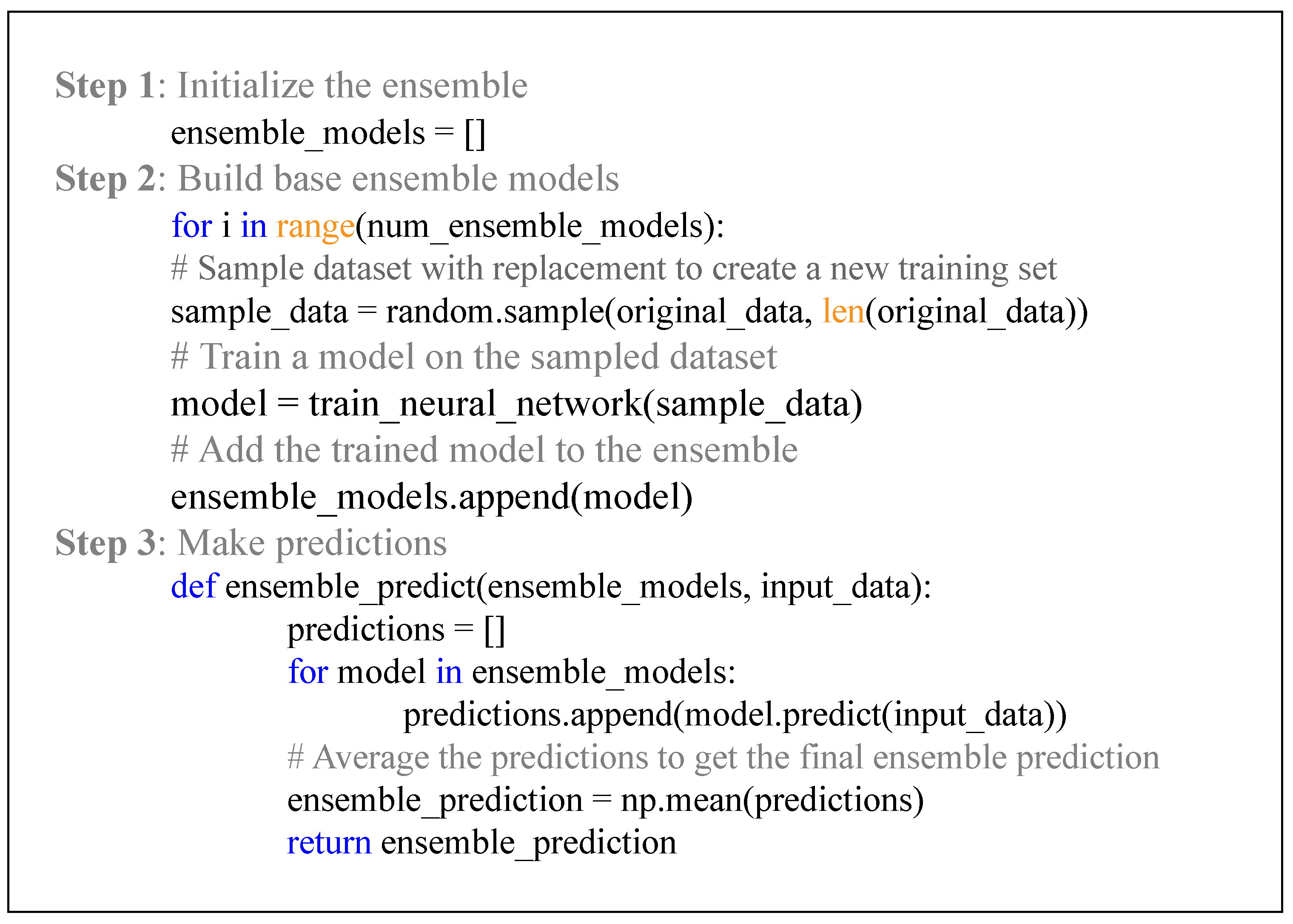
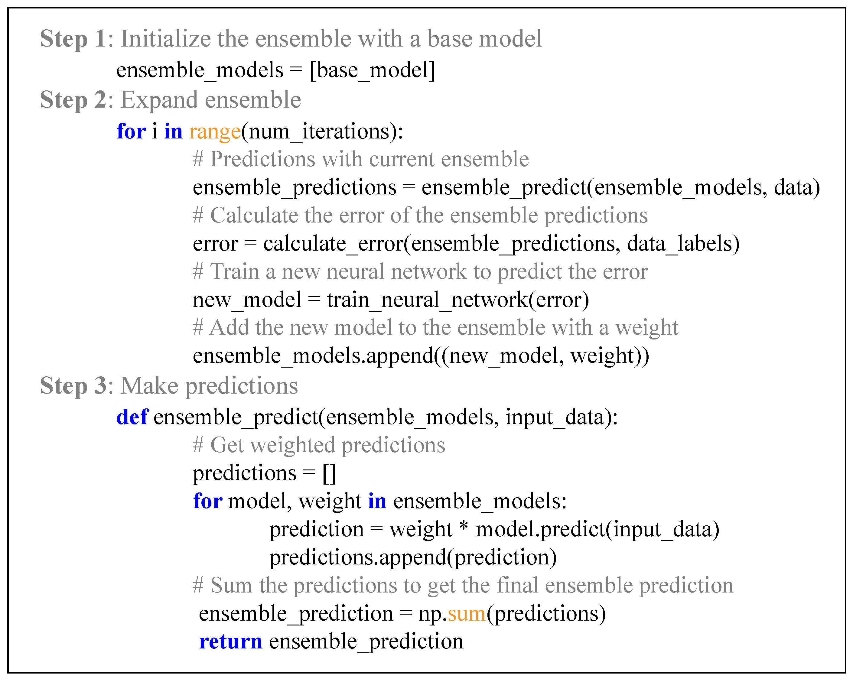
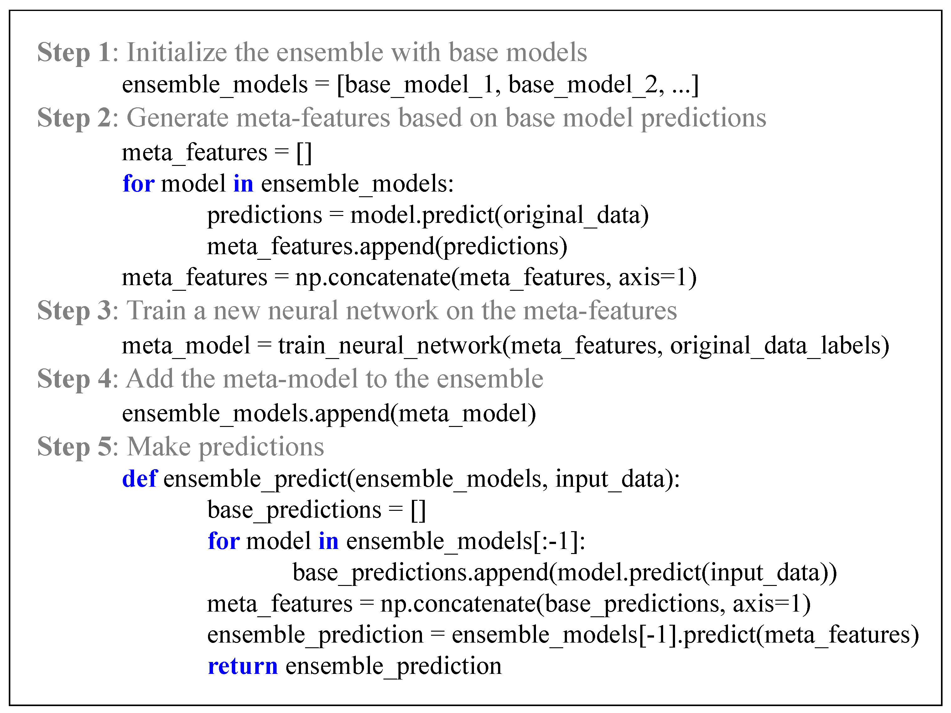
The present paper focuses on various approaches that can predict storm surge levels using ensemble neural networks. The challenges and limitations of accurately predicting peak water levels, which are often caused by complex interactions between ocean currents, winds, and atmospheric pressure systems, are also emphasized. Despite the limitations, supervised neural networks, specifically those utilizing the backpropagation technique, have proven to be a powerful tool for predicting storm surge levels, particularly for short-term forecasting. However, the accuracy of BPNN models can be limited by overfitting, which occurs when the model becomes too complex and fits the training data too closely. To address the limitations of single BPNN models, ensemble methods that combine multiple neural network models to improve accuracy and reduce overfitting are preferred. Ensemble methods involve generating multiple base learners (weak classifiers) and combining their predictions to create a strong learner. There are three leading meta-algorithms for combining weak learners: bootstrap aggregating (bagging), boosting, and sitting. Bagging involves generating multiple training datasets by randomly sampling from the original dataset with replacement, then training each base learner on a different dataset. Boosting involves iteratively training weak classifiers, with each subsequent model focusing on the samples that were misclassified by the previous model. Stacking involves training a meta-learner that combines the predictions of multiple base learners. As the networks grow larger, the importance of pruning and fine-tuning, as well as data preparation and wrangling, become unquestionable. Data preparation involves preprocessing and organizing raw data before training a group of neural networks together as an ensemble. The goal of this crucial step is to ensure that the input data are consistent, relevant, and suitable for use by the ensemble. The paper highlights different sources of input data type for storm surge prediction and the need for careful data preprocessing and wrangling to ensure accurate predictions. However, there is no one-size-fits-all approach for creating an ensemble of neural networks for predicting storm surge levels. Instead, it is essential to carefully evaluate the performance of different ensemble models and select the one that provides the best trade-off between bias and variance, accuracy, diversity, stability, generalization, and computational cost. Overall, the paper provides valuable insights into the use of ensemble methods for storm surge flood modeling, which can contribute to better predictions and preparedness for extreme weather events.

References

1. Heberger, M.; Cooley, H.; Herrera, P.; Gleick, P.H.; Moore, E. Potential impacts of increased coastal flooding in California due to sea-level rise. Clim. Chang. 2011, 109, 229–249. [Google Scholar] [CrossRef]
2. Woodruff, J.D.; Irish, J.L.; Camargo, S.J. Coastal flooding by tropical cyclones and sea-level rise. Nature 2013, 504, 44–52. [Google Scholar] [CrossRef] [PubMed]
3. Barooni, M.; Nezhad, S.K.; Ali, N.A.; Ashuri, T.; Sogut, D.V. Numerical study of ice-induced loads and dynamic response analysis for floating offshore wind turbines. Mar. Struct. 2022, 86, 103300. [Google Scholar] [CrossRef]
4. Cahoon, D.R.; Hensel, P.F.; Spencer, T.; Reed, D.J.; McKee, K.L.; Saintilan, N. Coastal wetland vulnerability to relative sea-level rise: Wetland elevation trends and process controls. In Wetlands and Natural Resource Management; Springer: Berlin/Heidelberg, Germany, 2006; pp. 271–292. [Google Scholar]
5. Dube, S.; Jain, I.; Rao, A.; Murty, T. Storm surge modelling for the Bay of Bengal and Arabian Sea. Nat. Hazards 2009, 51, 3–27. [Google Scholar] [CrossRef]
6. Hashemi, M.R.; Spaulding, M.L.; Shaw, A.; Farhadi, H.; Lewis, M. An efficient artificial intelligence model for prediction of tropical storm surge. Nat. Hazards 2016, 82, 471–491. [Google Scholar] [CrossRef]
7. Flowerdew, J.; Horsburgh, K.; Wilson, C.; Mylne, K. Development and evaluation of an ensemble forecasting system for coastal storm surges. Q. J. R. Meteorol. Soc. 2010, 136, 1444–1456. [Google Scholar] [CrossRef]
8. Lynett, P.J.; Gately, K.; Wilson, R.; Montoya, L.; Arcas, D.; Aytore, B.; Bai, Y.; Bricker, J.D.; Castro, M.J.; Cheung, K.F.; et al. Inter-model analysis of tsunami-induced coastal currents. Ocean. Model. 2017, 114, 14–32. [Google Scholar] [CrossRef]
9. Arabi, M.G.; Sogut, D.V.; Khosronejad, A.; Yalciner, A.C.; Farhadzadeh, A. A numerical and experimental study of local hydrodynamics due to interactions between a solitary wave and an impervious structure. Coast. Eng. 2019, 147, 43–62. [Google Scholar] [CrossRef]
10. Al Kajbaf, A.; Bensi, M. Application of surrogate models in estimation of storm surge: A comparative assessment. Appl. Soft Comput. 2020, 91, 106184. [Google Scholar] [CrossRef]
11. Qiao, C.; Myers, A.T.; Arwade, S.R. Validation and uncertainty quantification of metocean models for assessing hurricane risk. Wind. Energy 2020, 23, 220–234. [Google Scholar] [CrossRef]
12. Arns, A.; Dangendorf, S.; Jensen, J.; Talke, S.; Bender, J.; Pattiaratchi, C. Sea-level rise induced amplification of coastal protection design heights. Sci. Rep. 2017, 7, 40171. [Google Scholar] [CrossRef]
13. Weaver, R.J.; Slinn, D.N. Effect of wave forcing on storm surge. In Coastal Engineering 2004: (In 4 Volumes); World Scientific: Singapore, 2005; pp. 1532–1538. [Google Scholar]
14. Sweet, W.V.; Kopp, R.E.; Weaver, C.P.; Obeysekera, J.; Horton, R.M.; Thieler, E.R.; Zervas, C. Global and Regional Sea Level Rise Scenarios for the United States; Technical Report; National Oceanic and Atmospheric Administration: Washington, DC, USA, 2017.
15. Liu, Z.; Cheng, L.; Hao, Z.; Li, J.; Thorstensen, A.; Gao, H. A framework for exploring joint effects of conditional factors on compound floods. Water Resour. Res. 2018, 54, 2681–2696. [Google Scholar] [CrossRef]
16. Xi, D.; Lin, N. Understanding uncertainties in tropical cyclone rainfall hazard modeling using synthetic storms. J. Hydrometeorol. 2022, 23, 925–946. [Google Scholar] [CrossRef]
17. Dtissibe, F.Y.; Ari, A.A.A.; Titouna, C.; Thiare, O.; Gueroui, A.M. Flood forecasting based on an artificial neural network scheme. Nat. Hazards 2020, 104, 1211–1237. [Google Scholar] [CrossRef]
18. Velioglu, D. Advanced Two-and Three-Dimensional Tsunami Models: Benchmarking and Validation. Ph.D. Thesis, Middle East Technical University, Ankara, Turkey, 2017. [Google Scholar]
19. Chen, Y.; Li, J.; Xu, H. Improving flood forecasting capability of physically based distributed hydrological models by parameter optimization. Hydrol. Earth Syst. Sci. 2016, 20, 375–392. [Google Scholar] [CrossRef]
20. Agudelo-Otálora, L.M.; Moscoso-Barrera, W.D.; Paipa-Galeano, L.A.; Mesa-Sciarrotta, C. Comparación de modelos físicos y de inteligencia artificial para predicción de niveles de inundación. Tecnol. Cienc. Agua 2018, 9, 209–235. [Google Scholar] [CrossRef]
21. Zhang, Z.; Liang, J.; Zhou, Y.; Huang, Z.; Jiang, J.; Liu, J.; Yang, L. A multi-strategy-mode waterlogging-prediction framework for urban flood depth. Nat. Hazards Earth Syst. Sci. 2022, 22, 4139–4165. [Google Scholar] [CrossRef]
22. Oddo, P.C.; Lee, B.S.; Garner, G.G.; Srikrishnan, V.; Reed, P.M.; Forest, C.E.; Keller, K. Deep uncertainties in sea-level rise and storm surge projections: Implications for coastal flood risk management. Risk Anal. 2020, 40, 153–168. [Google Scholar] [CrossRef]
23. Ju, Y.; Lindbergh, S.; He, Y.; Radke, J.D. Climate-related uncertainties in urban exposure to sea level rise and storm surge flooding: A multi-temporal and multi-scenario analysis. Cities 2019, 92, 230–246. [Google Scholar] [CrossRef]
24. Makris, C.V.; Tolika, K.; Baltikas, V.N.; Velikou, K.; Krestenitis, Y.N. The impact of climate change on the storm surges of the Mediterranean Sea: Coastal sea level responses to deep depression atmospheric systems. Ocean. Model. 2023, 181, 102149. [Google Scholar] [CrossRef]
25. Camargo, S.J.; Barnston, A.G.; Zebiak, S.E. A statistical assessment of tropical cyclone activity in atmospheric general circulation models. Tellus A Dyn. Meteorol. Oceanogr. 2005, 57, 589–604. [Google Scholar] [CrossRef]
26. Tadesse, M.; Wahl, T.; Cid, A. Data-driven modeling of global storm surges. Front. Mar. Sci. 2020, 7, 260. [Google Scholar] [CrossRef]
27. Bevacqua, E.; Maraun, D.; Vousdoukas, M.; Voukouvalas, E.; Vrac, M.; Mentaschi, L.; Widmann, M. Higher probability of compound flooding from precipitation and storm surge in Europe under anthropogenic climate change. Sci. Adv. 2019, 5, eaaw5531. [Google Scholar] [CrossRef]
28. Jelesnianski, C.P. Numerical computations of storm surges without bottom stress. Mon. Weather Rev. 1966, 94, 379–394. [Google Scholar] [CrossRef]
29. Kim, Y.H. Assessment of coastal inundation due to storm surge under future sea-level rise conditions. J. Coast. Res. 2020, 95, 845–849. [Google Scholar] [CrossRef]
30. Seo, J.; Ku, H.; Cho, K.; Maeng, J.H.; Lee, H. Application of SLOSH in estimation of Typhoon-induced Storm Surges in the Coastal Region of South Korea. J. Coast. Res. 2018, 551–555. [Google Scholar] [CrossRef]
31. Dietrich, J.C.; Tanaka, S.; Westerink, J.J.; Dawson, C.N.; Luettich, R.; Zijlema, M.; Holthuijsen, L.H.; Smith, J.; Westerink, L.; Westerink, H. Performance of the unstructured-mesh, SWAN+ ADCIRC model in computing hurricane waves and surge. J. Sci. Comput. 2012, 52, 468–497. [Google Scholar] [CrossRef]
32. De Las Heras, M.; Burgers, G.; Janssen, P. Wave data assimilation in the WAM wave model. J. Mar. Syst. 1995, 6, 77–85. [Google Scholar] [CrossRef]
33. Bender, C.; Smith, J.M.; Kennedy, A.; Jensen, R. STWAVE simulation of Hurricane Ike: Model results and comparison to data. Coast. Eng. 2013, 73, 58–70. [Google Scholar] [CrossRef]
34. Booij, N.; Holthuijsen, L.; Ris, R. The “SWAN” wave model for shallow water. Coast. Eng. 1996, 668–676. [Google Scholar]
35. Reffitt, M.; Orescanin, M.M.; Massey, C.; Raubenheimer, B.; Jensen, R.E.; Elgar, S. Modeling storm surge in a small tidal two-inlet system. J. Waterw. Port Coast. Ocean. Eng. 2020, 146, 04020043. [Google Scholar] [CrossRef]
36. Ramos Valle, A.N.; Curchitser, E.N.; Bruyere, C.L.; Fossell, K.R. Simulating storm surge impacts with a coupled atmosphere-inundation model with varying meteorological forcing. J. Mar. Sci. Eng. 2018, 6, 35. [Google Scholar] [CrossRef]
37. Lee, J.W.; Irish, J.L.; Bensi, M.T.; Marcy, D.C. Rapid prediction of peak storm surge from tropical cyclone track time series using machine learning. Coast. Eng. 2021, 170, 104024. [Google Scholar] [CrossRef]
38. Smith, J.M.; Westerink, J.J.; Kennedy, A.B.; Taflanidis, A.A.; Cheung, K.F.; Smith, T.D. SWIMS Hawaii hurricane wave, surge, and runup inundation fast forecasting tool. In Proceedings of the Solutions to Coastal Disasters Conference, Anchorage, AK, USA, 25–29 June 2011; pp. 89–98. [Google Scholar]
39. Torres, M.J.; Nadal-Caraballo, N.C.; Ramos-Santiago, E.; Campbell, M.O.; Gonzalez, V.M.; Melby, J.A.; Taflanidis, A.A. StormSim-CHRPS: Coastal Hazards Rapid Prediction System. J. Coast. Res. 2020, 95, 1320–1325. [Google Scholar] [CrossRef]
40. Ishida, K.; Tsujimoto, G.; Ercan, A.; Tu, T.; Kiyama, M.; Amagasaki, M. Hourly-scale coastal sea level modeling in a changing climate using long short-term memory neural network. Sci. Total Environ. 2020, 720, 137613. [Google Scholar] [CrossRef] [PubMed]
41. Tebaldi, C.; Ranasinghe, R.; Vousdoukas, M.; Rasmussen, D.; Vega-Westhoff, B.; Kirezci, E.; Kopp, R.E.; Sriver, R.; Mentaschi, L. Extreme sea levels at different global warming levels. Nat. Clim. Chang. 2021, 11, 746–751. [Google Scholar] [CrossRef]
42. Ayyad, M.; Hajj, M.R.; Marsooli, R. Machine learning-based assessment of storm surge in the New York metropolitan area. Sci. Rep. 2022, 12, 19215. [Google Scholar] [CrossRef]
43. Tiggeloven, T.; Couasnon, A.; van Straaten, C.; Muis, S.; Ward, P.J. Exploring deep learning capabilities for surge predictions in coastal areas. Sci. Rep. 2021, 11, 17224. [Google Scholar] [CrossRef] [PubMed]
44. Žust, L.; Fettich, A.; Kristan, M.; Ličer, M. HIDRA 1.0: Deep-learning-based ensemble sea level forecasting in the northern Adriatic. Geosci. Model Dev. 2021, 14, 2057–2074. [Google Scholar] [CrossRef]
45. Ho, F.P.; Myers, V.A. Joint probability method of tide frequency analysis applied to Apalachicola Bay and St. George Sound, Florida; U.S. Department of Commerce, National Oceanic and Atmospheric Administration, National Weather Service, Office of Hydrology: Washington, DC, USA, 1975; Volume 18.
46. Feng, J.; Li, D.; Li, Y.; Liu, Q.; Wang, A. Storm surge variation along the coast of the Bohai Sea. Sci. Rep. 2018, 8, 11309. [Google Scholar] [CrossRef]
47. Ramos-Valle, A.N.; Curchitser, E.N.; Bruyère, C.L.; McOwen, S. Implementation of an artificial neural network for storm surge forecasting. J. Geophys. Res. Atmos. 2021, 126, e2020JD033266. [Google Scholar] [CrossRef]
48. Igarashi, Y.; Tajima, Y. Application of recurrent neural network for prediction of the time-varying storm surge. Coast. Eng. J. 2021, 63, 68–82. [Google Scholar] [CrossRef]
49. Kim, S.W.; Lee, A.; Mun, J. A surrogate modeling for storm surge prediction using an artificial neural network. J. Coast. Res. 2018, 866–870. [Google Scholar] [CrossRef]
50. Royston, S.; Lawry, J.; Horsburgh, K. A linguistic decision tree approach to predicting storm surge. Fuzzy Sets Syst. 2013, 215, 90–111. [Google Scholar] [CrossRef]
51. Bezuglov, A.; Blanton, B.; Santiago, R. Multi-output artificial neural network for storm surge prediction in north carolina. arXiv 2016, arXiv:1609.07378. [Google Scholar]
52. Bass, B.; Bedient, P. Surrogate modeling of joint flood risk across coastal watersheds. J. Hydrol. 2018, 558, 159–173. [Google Scholar] [CrossRef]
53. Tadesse, M.G.; Wahl, T. A database of global storm surge reconstructions. Sci. Data 2021, 8, 125. [Google Scholar] [CrossRef]
54. Palmer, M.; Domingues, C.; Slangen, A.; Dias, F.B. An ensemble approach to quantify global mean sea-level rise over the 20th century from tide gauge reconstructions. Environ. Res. Lett. 2021, 16, 044043. [Google Scholar] [CrossRef]
55. Bruneau, N.; Polton, J.; Williams, J.; Holt, J. Estimation of global coastal sea level extremes using neural networks. Environ. Res. Lett. 2020, 15, 074030. [Google Scholar] [CrossRef]
56. Chen, R.; Zhang, W.; Wang, X. Machine learning in tropical cyclone forecast modeling: A review. Atmosphere 2020, 11, 676. [Google Scholar] [CrossRef]
57. De Oliveira, M.M.; Ebecken, N.F.F.; De Oliveira, J.L.F.; de Azevedo Santos, I. Neural network model to predict a storm surge. J. Appl. Meteorol. Climatol. 2009, 48, 143–155. [Google Scholar] [CrossRef]
58. Taylor, A.A.; Glahn, B. Probabilistic guidance for hurricane storm surge. In Proceedings of the 19th Conference on Probability and Statistics, New Orleans, LA, USA, 21–24 January 2008; Volume 74. [Google Scholar]
59. Feng, X.; Ma, G.; Su, S.F.; Huang, C.; Boswell, M.K.; Xue, P. A multi-layer perceptron approach for accelerated wave forecasting in Lake Michigan. Ocean. Eng. 2020, 211, 107526. [Google Scholar] [CrossRef]
60. Deo, R.C.; Ghorbani, M.A.; Samadianfard, S.; Maraseni, T.; Bilgili, M.; Biazar, M. Multi-layer perceptron hybrid model integrated with the firefly optimizer algorithm for windspeed prediction of target site using a limited set of neighboring reference station data. Renew. Energy 2018, 116, 309–323. [Google Scholar] [CrossRef]
61. Kulkarni, P.A.; Dhoble, A.S.; Padole, P.M. Deep neural network-based wind speed forecasting and fatigue analysis of a large composite wind turbine blade. Proc. Inst. Mech. Eng. Part C J. Mech. Eng. Sci. 2019, 233, 2794–2812. [Google Scholar] [CrossRef]
62. Chattopadhyay, A.; Hassanzadeh, P.; Pasha, S. Predicting clustered weather patterns: A test case for applications of convolutional neural networks to spatio-temporal climate data. Sci. Rep. 2020, 10, 1317. [Google Scholar] [CrossRef] [PubMed]
63. Luo, Y.; Feng, A.; Li, H.; Li, D.; Wu, X.; Liao, J.; Zhang, C.; Zheng, X.; Pu, H. New deep learning method for efficient extraction of small water from remote sensing images. PLoS ONE 2022, 17, e0272317. [Google Scholar] [CrossRef]
64. Hunt, K.M.; Matthews, G.R.; Pappenberger, F.; Prudhomme, C. Using a long short-term memory (LSTM) neural network to boost river streamflow forecasts over the western United States. Hydrol. Earth Syst. Sci. 2022, 26, 5449–5472. [Google Scholar] [CrossRef]
65. Zilong, T.; Yubing, S.; Xiaowei, D. Spatial-temporal wave height forecast using deep learning and public reanalysis dataset. Appl. Energy 2022, 326, 120027. [Google Scholar] [CrossRef]
66. Varalakshmi, P.; Vasumathi, N.; Venkatesan, R. Tropical Cyclone prediction based on multi-model fusion across Indian coastal region. Prog. Oceanogr. 2021, 193, 102557. [Google Scholar] [CrossRef]
67. Sagi, O.; Rokach, L. Ensemble learning: A survey. Wiley Interdiscip. Rev. Data Min. Knowl. Discov. 2018, 8, e1249. [Google Scholar] [CrossRef]
68. Young, C.C.; Liu, W.C.; Hsieh, W.L. Predicting the water level fluctuation in an alpine lake using physically based, artificial neural network, and time series forecasting models. Math. Probl. Eng. 2015, 2015, 708204. [Google Scholar] [CrossRef]
69. Kim, S.; Matsumi, Y.; Pan, S.; Mase, H. A real-time forecast model using artificial neural network for after-runner storm surges on the Tottori coast, Japan. Ocean. Eng. 2016, 122, 44–53. [Google Scholar] [CrossRef]
70. Blake, E.S.; Zelinsky, D.A. National Hurricane Center Tropical Cyclone Report; Hurricane Harvey; National Hurricane Center, National Oceanographic and Atmospheric Association: Miami, FL, USA, 2017.
71. Qin, Y.; Su, C.; Chu, D.; Zhang, J.; Song, J. A Review of Application of Machine Learning in Storm Surge Problems. J. Mar. Sci. Eng. 2023, 11, 1729. [Google Scholar] [CrossRef]
72. Yu, Y.; Zhang, H.; Singh, V.P. Forward prediction of runoff data in data-scarce basins with an improved ensemble empirical mode decomposition (EEMD) model. Water 2018, 10, 388. [Google Scholar] [CrossRef]
73. Le, X.H.; Ho, H.V.; Lee, G.; Jung, S. Application of long short-term memory (LSTM) neural network for flood forecasting. Water 2019, 11, 1387. [Google Scholar] [CrossRef]
74. Liao, L.; Li, H.; Shang, W.; Ma, L. An empirical study of the impact of hyperparameter tuning and model optimization on the performance properties of deep neural networks. ACM Trans. Softw. Eng. Methodol. (TOSEM) 2022, 31, 1–40. [Google Scholar] [CrossRef]
75. Victoria, A.H.; Maragatham, G. Automatic tuning of hyperparameters using Bayesian optimization. Evol. Syst. 2021, 12, 217–223. [Google Scholar] [CrossRef]
76. Yu, T.; Zhu, H. Hyper-parameter optimization: A review of algorithms and applications. arXiv 2020, arXiv:2003.05689. [Google Scholar]
77. Hu, C.; Wu, Q.; Li, H.; Jian, S.; Li, N.; Lou, Z. Deep learning with a long short-term memory networks approach for rainfall-runoff simulation. Water 2018, 10, 1543. [Google Scholar] [CrossRef]
78. Zhang, X.q.; Jiang, S.q. Study on the application of BP neural network optimized based on various optimization algorithms in storm surge prediction. Proc. Inst. Mech. Eng. Part M J. Eng. Marit. Environ. 2022, 236, 539–552. [Google Scholar] [CrossRef]
79. Lee, T.L. Back-propagation neural network for the prediction of the short-term storm surge in Taichung harbor, Taiwan. Eng. Appl. Artif. Intell. 2008, 21, 63–72. [Google Scholar] [CrossRef]
80. Tsai, C.; You, C.; Chen, C. Storm-surge prediction at the Tanshui estuary: Development model for maximum storm surges. Nat. Hazards Earth Syst. Sci 2013, 1, 7333–7356. [Google Scholar]
81. Alzubaidi, L.; Zhang, J.; Humaidi, A.J.; Al-Dujaili, A.; Duan, Y.; Al-Shamma, O.; Santamaría, J.; Fadhel, M.A.; Al-Amidie, M.; Farhan, L. Review of deep learning: Concepts, CNN architectures, challenges, applications, future directions. J. Big Data 2021, 8, 1–74. [Google Scholar] [CrossRef] [PubMed]
82. Giffard-Roisin, S.; Yang, M.; Charpiat, G.; Kumler Bonfanti, C.; Kégl, B.; Monteleoni, C. Tropical cyclone track forecasting using fused deep learning from aligned reanalysis data. Front. Big Data 2020, 3, 1. [Google Scholar] [CrossRef]
83. Wang, T.; Liu, T.; Lu, Y. A hybrid multi-step storm surge forecasting model using multiple feature selection, deep learning neural network and transfer learning. Soft Comput. 2023, 27, 935–952. [Google Scholar] [CrossRef]
84. Weiss, K.; Khoshgoftaar, T.M.; Wang, D. A survey of transfer learning. J. Big Data 2016, 3, 1–40. [Google Scholar] [CrossRef]
85. Wu, W.; Westra, S.; Leonard, M. A basis function approach for exploring the seasonal and spatial features of storm surge events. Geophys. Res. Lett. 2017, 44, 7356–7365. [Google Scholar] [CrossRef]
86. Wolf, J.; Flather, R. Modelling waves and surges during the 1953 storm. Philos. Trans. R. Soc. A Math. Phys. Eng. Sci. 2005, 363, 1359–1375. [Google Scholar] [CrossRef] [PubMed]
87. Feng, J.; von Storch, H.; Jiang, W.; Weisse, R. Assessing changes in extreme sea levels along the coast of C hina. J. Geophys. Res. Ocean. 2015, 120, 8039–8051. [Google Scholar] [CrossRef]
88. Bloemendaal, N.; Haigh, I.D.; de Moel, H.; Muis, S.; Haarsma, R.J.; Aerts, J.C. Generation of a global synthetic tropical cyclone hazard dataset using STORM. Sci. Data 2020, 7, 40. [Google Scholar] [CrossRef]
89. Adhikari, R.; Agrawal, R. A homogeneous ensemble of artificial neural networks for time series forecasting. arXiv 2013, arXiv:1302.6210. [Google Scholar]
90. Guan, H.; Mokadam, L.K.; Shen, X.; Lim, S.H.; Patton, R. Fleet: Flexible efficient ensemble training for heterogeneous deep neural networks. Proc. Mach. Learn. Syst. 2020, 2, 247–261. [Google Scholar]
91. Zhou, Z.H.; Zhou, Z.H. Ensemble Learning; Springer: Berlin/Heidelberg, Germany, 2021. [Google Scholar]
92. Zhou, Z.H.; Wu, J.; Tang, W. Ensembling neural networks: Many could be better than all. Artif. Intell. 2002, 137, 239–263. [Google Scholar] [CrossRef]
93. Ghojogh, B.; Crowley, M. The theory behind overfitting, cross validation, regularization, bagging, and boosting: Tutorial. arXiv 2019, arXiv:1905.12787. [Google Scholar]
94. Brodeur, Z.P.; Herman, J.D.; Steinschneider, S. Bootstrap aggregation and cross-validation methods to reduce overfitting in reservoir control policy search. Water Resour. Res. 2020, 56, e2020WR027184. [Google Scholar] [CrossRef]
95. Altman, N.; Krzywinski, M. Ensemble methods: Bagging and random forests. Nat. Methods 2017, 14, 933–935. [Google Scholar] [CrossRef]
96. Dietterich, T.G. Ensemble methods in machine learning. In Proceedings of the Multiple Classifier Systems: First International Workshop, MCS 2000, Cagliari, Italy, 21–23 June 2000; pp. 1–15. [Google Scholar]
97. Cassales, G.; Gomes, H.; Bifet, A.; Pfahringer, B.; Senger, H. Improving the performance of bagging ensembles for data streams through mini-batching. Inf. Sci. 2021, 580, 260–282. [Google Scholar] [CrossRef]
98. Maxwell, A.E.; Warner, T.A.; Fang, F. Implementation of machine-learning classification in remote sensing: An applied review. Int. J. Remote Sens. 2018, 39, 2784–2817. [Google Scholar] [CrossRef]
99. Zounemat-Kermani, M.; Batelaan, O.; Fadaee, M.; Hinkelmann, R. Ensemble machine learning paradigms in hydrology: A review. J. Hydrol. 2021, 598, 126266. [Google Scholar] [CrossRef]
100. Elith, J.; Leathwick, J.R.; Hastie, T. A working guide to boosted regression trees. J. Anim. Ecol. 2008, 77, 802–813. [Google Scholar] [CrossRef]
101. Freund, Y.; Schapire, R.E. A decision-theoretic generalization of on-line learning and an application to boosting. J. Comput. Syst. Sci. 1997, 55, 119–139. [Google Scholar] [CrossRef]
102. Lawry, J.; He, H. Linguistic decision trees for fusing tidal surge forecasting models. In Combining Soft Computing and Statistical Methods in Data Analysis; Springer: Berlin/Heidelberg, Germany, 2010; pp. 403–410. [Google Scholar]
103. Bentéjac, C.; Csörgo, A.; Martínez-Muñoz, G. A comparative analysis of gradient boosting algorithms. Artif. Intell. Rev. 2021, 54, 1937–1967. [Google Scholar] [CrossRef]
104. Chen, T.; Guestrin, C. Xgboost: A scalable tree boosting system. In Proceedings of the 22nd ACM Sigkdd International Conference on Knowledge Discovery and Data Mining, San Francisco, CA, USA, 13–17 August 2016; pp. 785–794. [Google Scholar]
105. Drucker, H. Improving regressors using boosting techniques. In Proceedings of the Fourteenth International Conference on Machine Learning (ICML 1997), Nashville, TN, USA, 8–12 July 1997; Volume 97, pp. 107–115. [Google Scholar]
106. Muis, S.; Apecechea, M.I.; Dullaart, J.; de Lima Rego, J.; Madsen, K.S.; Su, J.; Yan, K.; Verlaan, M. A high-resolution global dataset of extreme sea levels, tides, and storm surges, including future projections. Front. Mar. Sci. 2020, 7, 263. [Google Scholar] [CrossRef]
107. Sesmero, M.P.; Ledezma, A.I.; Sanchis, A. Generating ensembles of heterogeneous classifiers using stacked generalization. Wiley Interdiscip. Rev. Data Min. Knowl. Discov. 2015, 5, 21–34. [Google Scholar] [CrossRef]
108. Barton, M.; Lennox, B. Model stacking to improve prediction and variable importance robustness for soft sensor development. Digit. Chem. Eng. 2022, 3, 100034. [Google Scholar] [CrossRef]
109. Džeroski, S.; Ženko, B. Is combining classifiers with stacking better than selecting the best one? Mach. Learn. 2004, 54, 255–273. [Google Scholar] [CrossRef]
110. Breiman, L. Stacked regressions. Mach. Learn. 1996, 24, 49–64. [Google Scholar] [CrossRef]
111. Zucco, C. Multiple Learners Combination: Stacking. In Encyclopedia of Bioinformatics and Computational Biology; Ranganathan, S., Gribskov, M., Nakai, K., Schönbach, C., Eds.; Academic Press: Oxford, UK, 2019; pp. 536–538. [Google Scholar] [CrossRef]
112. Sill, J.; Takács, G.; Mackey, L.; Lin, D. Feature-weighted linear stacking. arXiv 2009, arXiv:0911.0460. [Google Scholar]
113. Young, S.; Abdou, T.; Bener, A. Deep super learner: A deep ensemble for classification problems. In Proceedings of the Advances in Artificial Intelligence: 31st Canadian Conference on Artificial Intelligence, Canadian AI 2018, Toronto, ON, Canada, 8–11 May 2018; pp. 84–95. [Google Scholar]
114. Wolpert, D.H. Stacked generalization. Neural Netw. 1992, 5, 241–259. [Google Scholar] [CrossRef]
115. Ayyad, M.; Orton, P.M.; El Safty, H.; Chen, Z.; Hajj, M.R. Ensemble forecast for storm tide and resurgence from Tropical Cyclone Isaias. Weather. Clim. Extrem. 2022, 38, 100504. [Google Scholar] [CrossRef]
116. Kim, S.W.; Melby, J.A.; Nadal-Caraballo, N.C.; Ratcliff, J. A time-dependent surrogate model for storm surge prediction based on an artificial neural network using high-fidelity synthetic hurricane modeling. Nat. Hazards 2015, 76, 565–585. [Google Scholar] [CrossRef]
117. Guo, T. Hurricane Damage Prediction based on Convolutional Neural Network Models. In Proceedings of the 2021 2nd International Conference on Artificial Intelligence and Computer Engineering (ICAICE), Hangzhou, China, 5–7 November 2021; pp. 298–302. [Google Scholar]
118. Gebrehiwot, A.; Hashemi-Beni, L.; Thompson, G.; Kordjamshidi, P.; Langan, T.E. Deep convolutional neural network for flood extent mapping using unmanned aerial vehicles data. Sensors 2019, 19, 1486. [Google Scholar] [CrossRef]
119. Accarino, G.; Chiarelli, M.; Fiore, S.; Federico, I.; Causio, S.; Coppini, G.; Aloisio, G. A multi-model architecture based on Long Short-Term Memory neural networks for multi-step sea level forecasting. Future Gener. Comput. Syst. 2021, 124, 1–9. [Google Scholar] [CrossRef]
120. Kaur, S.; Gupta, S.; Singh, S.; Koundal, D.; Zaguia, A. Convolutional neural network based hurricane damage detection using satellite images. Soft Comput. 2022, 26, 7831–7845. [Google Scholar] [CrossRef]
121. Korzh, O.; Joaristi, M.; Serra, E. Convolutional neural network ensemble fine-tuning for extended transfer learning. In Proceedings of the Big Data–BigData 2018: 7th International Congress, Held as Part of the Services Conference Federation, SCF 2018, Seattle, WA, USA, 25–30 June 2018; pp. 110–123. [Google Scholar]
122. Becherer, N.; Pecarina, J.; Nykl, S.; Hopkinson, K. Improving optimization of convolutional neural networks through parameter fine-tuning. Neural Comput. Appl. 2019, 31, 3469–3479. [Google Scholar] [CrossRef]
123. Blalock, D.; Gonzalez Ortiz, J.J.; Frankle, J.; Guttag, J. What is the state of neural network pruning? Proc. Mach. Learn. Syst. 2020, 2, 129–146. [Google Scholar]
124. Araghinejad, S.; Azmi, M.; Kholghi, M. Application of artificial neural network ensembles in probabilistic hydrological forecasting. J. Hydrol. 2011, 407, 94–104. [Google Scholar] [CrossRef]
125. Chen, W.; Hong, H.; Li, S.; Shahabi, H.; Wang, Y.; Wang, X.; Ahmad, B.B. Flood susceptibility modelling using novel hybrid approach of reduced-error pruning trees with bagging and random subspace ensembles. J. Hydrol. 2019, 575, 864–873. [Google Scholar] [CrossRef]
126. Du, L.; Gao, R.; Suganthan, P.N.; Wang, D.Z. Bayesian optimization based dynamic ensemble for time series forecasting. Inf. Sci. 2022, 591, 155–175. [Google Scholar] [CrossRef]
127. Pham, B.T.; Jaafari, A.; Nguyen-Thoi, T.; Van Phong, T.; Nguyen, H.D.; Satyam, N.; Masroor, M.; Rehman, S.; Sajjad, H.; Sahana, M.; et al. Ensemble machine learning models based on Reduced Error Pruning Tree for prediction of rainfall-induced landslides. Int. J. Digit. Earth 2021, 14, 575–596. [Google Scholar] [CrossRef]
128. Rooney, N.; Patterson, D.; Nugent, C. Reduced ensemble size stacking [ensemble learning]. In Proceedings of the 16th IEEE International Conference on Tools with Artificial Intelligence, Boca Raton, FL, USA, 15–17 November 2004; pp. 266–271. [Google Scholar]
129. Naftaly, U.; Intrator, N.; Horn, D. Optimal ensemble averaging of neural networks. Netw. Comput. Neural Syst. 1997, 8, 283. [Google Scholar] [CrossRef]
130. Huang, W.; Hong, H.; Bian, K.; Zhou, X.; Song, G.; Xie, K. Improving deep neural network ensembles using reconstruction error. In Proceedings of the 2015 International Joint Conference on Neural Networks (IJCNN), Killarney, Ireland, 12–17 July 2015; pp. 1–7. [Google Scholar]
131. Zeng, X.; Yeung, D.S. Hidden neuron pruning of multilayer perceptrons using a quantified sensitivity measure. Neurocomputing 2006, 69, 825–837. [Google Scholar] [CrossRef]
132. Smith, C.; Jin, Y. Evolutionary multi-objective generation of recurrent neural network ensembles for time series prediction. Neurocomputing 2014, 143, 302–311. [Google Scholar] [CrossRef]
133. Shahhosseini, M.; Hu, G.; Pham, H. Optimizing ensemble weights and hyperparameters of machine learning models for regression problems. Mach. Learn. Appl. 2022, 7, 100251. [Google Scholar] [CrossRef]
134. Palaniswamy, S.K.; Venkatesan, R. Hyperparameters tuning of ensemble model for software effort estimation. J. Ambient. Intell. Humaniz. Comput. 2021, 12, 6579–6589. [Google Scholar] [CrossRef]
135. Snoek, J.; Larochelle, H.; Adams, R.P. Practical bayesian optimization of machine learning algorithms. In Advances in Neural Information Processing Systems; Curran Associates, Inc.: Red Hook, NY, USA, 2012; Volume 25. [Google Scholar]
136. Wu, J.; Chen, X.Y.; Zhang, H.; Xiong, L.D.; Lei, H.; Deng, S.H. Hyperparameter optimization for machine learning models based on Bayesian optimization. J. Electron. Sci. Technol. 2019, 17, 26–40. [Google Scholar]
137. Priyadarshini, I.; Cotton, C. A novel LSTM–CNN–grid search-based deep neural network for sentiment analysis. J. Supercomput. 2021, 77, 13911–13932. [Google Scholar] [CrossRef] [PubMed]
138. Huang, G.B.; Chen, L. Enhanced random search based incremental extreme learning machine. Neurocomputing 2008, 71, 3460–3468. [Google Scholar] [CrossRef]
139. Agnihotri, A.; Batra, N. Exploring bayesian optimization. Distill 2020, 5, e26. [Google Scholar] [CrossRef]
140. Zhou, J.; Peng, T.; Zhang, C.; Sun, N. Data pre-analysis and ensemble of various artificial neural networks for monthly streamflow forecasting. Water 2018, 10, 628. [Google Scholar] [CrossRef]
141. Aloysius, N.; Geetha, M. A review on deep convolutional neural networks. In Proceedings of the 2017 International Conference on Communication and Signal Processing (ICCSP), Melmaruvathur, India, 6–8 April 2017; pp. 0588–0592. [Google Scholar]
142. Kiranyaz, S.; Avci, O.; Abdeljaber, O.; Ince, T.; Gabbouj, M.; Inman, D.J. 1D convolutional neural networks and applications: A survey. Mech. Syst. Signal Process. 2021, 151, 107398. [Google Scholar] [CrossRef]
143. Trice, A.; Robbins, C.; Philip, N.; Rumsey, M. Challenges and Opportunities for Ocean Data to Advance Conservation and Management; Ocean Conservancy: Washington, DC, USA, 2021. [Google Scholar]
144. Velioglu Sogut, D.; Yalciner, A.C. Performance comparison of NAMI DANCE and FLOW-3D® models in tsunami propagation, inundation and currents using NTHMP benchmark problems. Pure Appl. Geophys. 2019, 176, 3115–3153. [Google Scholar] [CrossRef]
145. Costa, W.; Idier, D.; Rohmer, J.; Menendez, M.; Camus, P. Statistical prediction of extreme storm surges based on a fully supervised weather-type downscaling model. J. Mar. Sci. Eng. 2020, 8, 1028. [Google Scholar] [CrossRef]
146. Cialone, M.A.; Massey, T.C.; Anderson, M.E.; Grzegorzewski, A.S.; Jensen, R.E.; Cialone, A.; Mark, D.J.; Pevey, K.C.; Gunkel, B.L.; McAlpin, T.O.; et al. North Atlantic Coast Comprehensive Study (NACCS) Coastal Storm Model Simulations: Waves and Water Levels; US Army Engineer Research and Development Center, Coastal and Hydraulics Laboratory: Vicksburg, MS, USA, 2015. [Google Scholar]
147. Yang, C.; Leonelli, F.E.; Marullo, S.; Artale, V.; Beggs, H.; Nardelli, B.B.; Chin, T.M.; De Toma, V.; Good, S.; Huang, B.; et al. Sea surface temperature intercomparison in the framework of the Copernicus Climate Change Service (C3S). J. Clim. 2021, 34, 5257–5283. [Google Scholar] [CrossRef]
148. Hersbach, H. Decomposition of the continuous ranked probability score for ensemble prediction systems. Weather. Forecast. 2000, 15, 559–570. [Google Scholar] [CrossRef]
149. Wallendorf, L.; Cox, D.T. Coastal Structures and Solutions to Coastal Disasters 2015: Tsunamis; American Society of Civil Engineers: Reston, VA, USA, 2017. [Google Scholar]
150. Conver, A.; Sepanik, J.; Louangsaysongkham, B.; Miller, S. Sea, Lake, and Overland Surges from Hurricanes (SLOSH) Basin Development Handbook v2.0; NOAA/NWS/Meteorological Development Laboratory: Silver Springs, MD, USA, 2008.
151. Miller, A.; Luscher, A. NOAA’s national water level observation network (NWLON). J. Oper. Oceanogr. 2019, 12, S57–S66. [Google Scholar] [CrossRef]
152. Raschka, S. Python Machine Learning; Packt Publishing Ltd.: Birmingham, UK, 2015. [Google Scholar]
153. Yang, H. Data preprocessing. In Data Mining: Concepts and Techniques; Pennsylvania State University, CiteSeerX: State College, PA, USA, 2018. [Google Scholar]
154. Knapp, K.R.; Kruk, M.C.; Levinson, D.H.; Diamond, H.J.; Neumann, C.J. The International Best Track Archive for Climate Stewardship (IBTrACS). Bull. Am. Meteorol. Soc. 2010, 91, 363–376. [Google Scholar] [CrossRef]
155. Knapp, K.R.; Diamond, H.J.; Kossin, J.P.; Kruk, M.C.; Schreck, C.J. International Best Track Archive for Climate Stewardship (IBTrACS) Project; Version 4; NOAA National Centers for Environmental Information: Asheville, NC, USA, 2018. [CrossRef]
156. NOAA National Data Buoy Center. Meteorological and Oceanographic Data Collected from the National Data Buoy Center Coastal-Marine Automated Network (C-MAN) and Moored (Weather) Buoys; NOAA National Centers for Environmental Information, Dataset: Port Aransas, TX, USA, 1971.
157. Adebisi, N.; Balogun, A.L.; Min, T.H.; Tella, A. Advances in estimating Sea Level Rise: A review of tide gauge, satellite altimetry and spatial data science approaches. Ocean. Coast. Manag. 2021, 208, 105632. [Google Scholar] [CrossRef]
158. Kyprioti, A.P.; Taflanidis, A.A.; Plumlee, M.; Asher, T.G.; Spiller, E.; Luettich, R.A.; Blanton, B.; Kijewski-Correa, T.L.; Kennedy, A.; Schmied, L. Improvements in storm surge surrogate modeling for synthetic storm parameterization, node condition classification and implementation to small size databases. Nat. Hazards 2021, 109, 1349–1386. [Google Scholar] [CrossRef]
159. Queipo, N.V.; Nava, E. A gradient boosting approach with diversity promoting measures for the ensemble of surrogates in engineering. Struct. Multidiscip. Optim. 2019, 60, 1289–1311. [Google Scholar] [CrossRef]
160. Freeman, J.; Velic, M.; Colberg, F.; Greenslade, D.; Divakaran, P.; Kepert, J. Development of a tropical storm surge prediction system for Australia. J. Mar. Syst. 2020, 206, 103317. [Google Scholar] [CrossRef]
161. Beuzen, T.; Goldstein, E.B.; Splinter, K.D. Ensemble models from machine learning: An example of wave runup and coastal dune erosion. Nat. Hazards Earth Syst. Sci. 2019, 19, 2295–2309. [Google Scholar] [CrossRef]
162. Goodarzi, L.; Banihabib, M.E.; Roozbahani, A. A decision-making model for flood warning system based on ensemble forecasts. J. Hydrol. 2019, 573, 207–219. [Google Scholar] [CrossRef]
163. Chang, L.C.; Amin, M.Z.M.; Yang, S.N.; Chang, F.J. Building ANN-based regional multi-step-ahead flood inundation forecast models. Water 2018, 10, 1283. [Google Scholar] [CrossRef]
164. Neal, B.; Mittal, S.; Baratin, A.; Tantia, V.; Scicluna, M.; Lacoste-Julien, S.; Mitliagkas, I. A modern take on the bias-variance tradeoff in neural networks. arXiv 2018, arXiv:1810.08591. [Google Scholar]
165. Ganaie, M.A.; Hu, M.; Malik, A.; Tanveer, M.; Suganthan, P. Ensemble deep learning: A review. Eng. Appl. Artif. Intell. 2022, 115, 105151. [Google Scholar] [CrossRef]
166. James, G.; Witten, D.; Hastie, T.; Tibshirani, R. An Introduction to Statistical Learning; Springer: Berlin/Heidelberg, Germany, 2013; Volume 112. [Google Scholar]
167. Ortega, L.A.; Cabañas, R.; Masegosa, A. Diversity and generalization in neural network ensembles. In Proceedings of the International Conference on Artificial Intelligence and Statistics, Valencia, Spain, 28–30 March 2022; pp. 11720–11743. [Google Scholar]
168. Tsymbal, A.; Pechenizkiy, M.; Cunningham, P. Diversity in search strategies for ensemble feature selection. Inf. Fusion 2005, 6, 83–98. [Google Scholar] [CrossRef]
169. Dutta, H. Measuring Diversity in Regression Ensembles. In Proceedings of the ICAI, Las Vegas, NV, USA, 13–16 July 2009; Volume 9, p. 17. [Google Scholar]
170. Horsburgh, K.; Flowerdew, J. Real-Time Coastal Flood Forecasting. In Applied Uncertainty Analysis for Flood Risk Management; World Scientific Publishing Co., Pte. Ltd.: London, UK, 2014; pp. 538–562. [Google Scholar]
171. Murphy, A.H. Skill scores based on the mean square error and their relationships to the correlation coefficient. Mon. Weather Rev. 1988, 116, 2417–2424. [Google Scholar] [CrossRef]
172. Tonani, M.; Pinardi, N.; Fratianni, C.; Pistoia, J.; Dobricic, S.; Pensieri, S.; De Alfonso, M.; Nittis, K. Mediterranean Forecasting System: Forecast and analysis assessment through skill scores. Ocean. Sci. 2009, 5, 649–660. [Google Scholar] [CrossRef]
Figure 1. (a) Best track positions and storm surge predictions from the empirical CHRPS model compared to water level observations from select NOAA tide gauge and storm surge predictions from operational ADCIRC simulations performed at CHL [39]. (b) Winds. (c) Hourly heights. (d) Barometric pressure. (e) Air temperature. (f) Sea surface temperature in Aransas Wildlife Refuge station, TX, for Hurricane Harvey (August 2017).
Jmse 11 02154 g001aJmse 11 02154 g001b
Figure 2. Flow diagram of transfer learning in NN, including the reuse of a pre-trained model on a new problem.
Jmse 11 02154 g002
Figure 3. Flow diagram of transfer learning in NN involving the reuse of a pre-trained model on a new problem.
Jmse 11 02154 g003
Figure 4. A general scheme of the bagging ensemble approach.
Jmse 11 02154 g004
Figure 5. A simplified pseudo-code of an ensemble learning algorithm for bagging.
Jmse 11 02154 g005
Figure 6. A general schematic of the boosting ensemble approach.
Jmse 11 02154 g006
Figure 7. A simplified pseudo-code of an ensemble learning algorithm for boosting.
Jmse 11 02154 g007
Figure 8. A general scheme of the stacking ensemble approach.
Jmse 11 02154 g008
Figure 9. A simplified pseudo-code of ensemble learning algorithm for stacking.
Jmse 11 02154 g009
Figure 10. Qualitative assessment of studies numbered 1 to 6 from Table 2.
Jmse 11 02154 g010
Figure 11. General process of pruning and fine-tuning in a neural network ensemble.
Jmse 11 02154 g011