Influence of Wave–Current Interaction on a Cyclone-Induced Storm Surge Event in the Ganges–Brahmaputra–Meghna Delta: Part 1—Effects on Water Level

Abstract

The Ganges–Brahmaputra–Meghna Delta (GBMD) located in the head of the Bay of Bengal is regularly affected by severe tropical cyclones frequently. The GBMD covers the Bangladesh coast, which is one of the most vulnerable areas in the world due to cyclone-induced storm surges. More than 30% of the total country’s population lives on the Bangladesh coast. Hence, it is crucial to understand the underlying processes that modulate the storm surge height in the GBMD. A barotropic numerical 3D model setup is established by using Delft3D and SWAN to investigate a cyclone-induced storm surge event. The model is calibrated and validated for Cyclone Sidr in 2007 and applied to six idealized cyclonic scenarios. Numerical experiments with different coupling configurations are performed to distinguish the contribution of wind, tides, waves, and wave–current interactions (WCI) on the storm surge height. Results show that the wind-driven setup is the dominant contributor to the storm surge height during cyclonic events. Based on the tidal phase and wind direction, the interaction between tide and wind can increase or decrease the magnitude of the storm surge height. Finally, considering the wind-driven wave may increase the surge height up to 0.3 m along the coastline through a strong wave setup.

1. Introduction

Coastal water variation depends on many factors including wind waves, storm surges, and ocean circulation. Surface water level modulation in both shallow and deep oceans is strongly influenced by different non-linear interaction processes including tide-surge interaction and wave–current interaction. The tide-surge interaction is a well-known factor that limits the ability of numerical models to accurately reproduce observed variations in mean water levels under extreme weather conditions, particularly in shallow areas [1]. Several studies [2,3,4,5,6] suggest that the discrepancy between model results and observations is due to the influence of wave setup and setdown arising from wave breaking. There are several studies focusing on wave–current interaction [7,8,9,10]. These studies demonstrate that wind waves can indirectly affect the coastal ocean circulation by enhancing wind stress [11] and by modulating the bed friction coefficient [12,13]. Xie et al. [9,10] reported that the wave–current interaction significantly influences the overall circulations in coastal regions by modifying surface and bottom stresses. Radiation stress is a source of momentum flux between surface waves and underlying ocean currents and is proportional to wave energy density [14,15]. The momentum flux transfer from wind waves to the water column is more evident during wave propagation from deep to shallow water, particularly by the gradient of radiation stress [16]. Water levels and currents have a complex influence on wave height through distinct physical processes. Significant wave height in shallow regions is strongly modulated by time-varying water depth. Furthermore, ocean currents accelerate or decelerate the energy transfer from surface winds to surface waves outside the estuary based on the orientation of the current and the waves [17,18,19]. The wave–current interaction mechanisms generally consist of wave–current bottom stress, wave radiation stress, wave dissipation, vertical transfer to the mean moment equation (known as form drag), Stokes drift velocities, current advection, and refraction of wave energy [20,21,22]. The wave–current interactions also depend on various factors such as continental shelf geometry [23], bathymetry [24], coastal morphology [25], and the path of cyclones [26]. A numerical study on the Irish sea demonstrates that considering the wave–current interactions in model simulations generates 20% larger high-water wave heights in some regions [27]. More recently, Zheng et al. [28] show that wave setup is strongly influenced by the radiation stress through the bathymetry and water depth based on performed laboratory experiments. The results also demonstrate the reduction of wave setup on the reef flat due to wave–current interaction with the presence of a strong onshore current. Another numerical study [29] on the southwest of Bohai Bay, China also shows that the wave setup is strongly affected by the local bottom slope, water depth, and radiation stress gradient. The study reports a 15% decrease in mean current velocity by wave-enhanced bottom roughness, and the influence of momentum transfer from wave to current is non-negligible. Several recent studies [27,30,31,32,33,34,35] carried out across the world investigate wave–current interactions during tropical cyclone conditions and illustrate the spatially varying influence of wave–current interactions on wave setup and total surge height. Therefore, the present study focuses on investigating the role of wave–current interactions on the storm surge height generation under tropical cyclonic conditions on the Bangladesh coast.

A large number of TCs form in the BoB during the pre-monsoon (May–June) and post-monsoon (October–December) seasons when favorable meteorological conditions for TC formation prevail [36]. Almost one-sixth of tropical cyclones that develop in the BoB make landfall in the Ganges–Brahmaputra–Meghna delta (GBMD [37]. The GBMD is located at the head of the Bay of Bengal (BoB), a semi-enclosed basin in the northeastern Indian Ocean, which exhibits unique geographic and hydrographic characteristics. Due to the low land elevation above mean sea level, the GBMD is vulnerable to frequent coastal and riverine flooding. In addition, the TC-induced storm surge accentuates the flooding conditions in coastal areas, posing a threat to the infrastructure, biodiversity, and the large population living in coastal regions. Storm surge events can be severe in Bangladesh because of the shape and characteristics of the coastline. The tangential wind of the TC drives the seawater northward from the south which generates the storm surge. The presence of the wide continental shelf in the eastern part of the Bangladesh coastline amplifies the storm surge when propagating from the deep ocean to shallower water [38,39]. Several recent cyclones, including Sidr, Aila, Roanu, and Amphan produced heavy flooding and caused a large extent of devastation to life and property. Therefore, it is vital to understand the mechanisms behind the cyclone-induced storm surge event in the GBMD to improve surge height prediction and provide better quality guidance to coastal disaster management.

Many numerical modeling studies have investigated storm surges in the Bay of Bengal [40,41,42,43,44,45,46,47,48,49]. All these studies demonstrate that shallow-water numerical models can reproduce the order of magnitude of maximum observed storm surges. During Cyclone Sidr in 2007, the IIT-D (Indian Institute of Technology—Delhi) storm surge model [50] was applied as a part of the early-warning system and showed maximum water level predictive capability with relatively good accuracy that helped to save lives [49]. Despite these achievements, numerical models struggle to reproduce patterns of coastal flooding both in space and time due to several challenges such as lack of high-quality water level records, uncertainties related to the cyclonic parameter, and lack of high-resolution bathymetric data in the shallow area. The storm surge modeling challenges in the GBMD are discussed in detail by Krien et al. [49].

One key challenge for storm surge modeling in the delta region is the lack of high-quality verification data. The lack of high-quality water level records during cyclones, bathymetric data in shallow areas, and observations of cyclonic parameters such as the maximum wind speed, and radius of maximum wind speed contribute to errors in model results. Moreover, the contribution of waves in hydrodynamic models has been mostly ignored by researchers in the GBMD, with the notable exception of Deb and Ferreira [39] and Krien et al. [49]. During TC events, the wind-induced stress at the ocean-atmosphere interface is expected to be the dominant mechanism for storm surge generation over coastal zones bordered by broad and shallow shelves [51,52,53]. Furthermore, currents and waves can interact with each other during a cyclonic event. This interaction depends on the magnitudes of each of the currents and waves. The storm surge, tides, and currents will have a significant effect on the wavefield only if their strengths are sufficient to interact [54]. These wave processes can influence the coastal hydrodynamic conditions in two ways: (i) wave setup during cyclones that contributes significantly to storm surge and inundation (ii) Wave–current interaction increases the bottom friction and causes an increase in the bottom stress [54]. The current can influence the wave by modifying the wave characteristics through refraction, bottom friction, and blocking [55]. Moreover, the mean flow will be affected by the addition of momentum and mass fluxes. The depth felt by the waves also changes with variations in water level in the coastal region, thereby modifying the shallow water effects on the waves [56]. Several studies [34,54] on cyclones making landfall on India’s eastern coast include wave effects in the models. These studies demonstrate that a significant portion (0.25 m, 20% of the total surge height during cyclone Hudhud) of the storm surge height can result from the wave setup. However, the contribution of the wave setup and wave–current interactions in the storm surge height in the GBMD is yet to be explored.

The physical environment of the coastal regions is modulated by the mutual interaction between physical processes, such as tides, waves, and currents [57]. Depending on the tidal phase, wind- and wave-induced currents can reinforce or interfere with tidal currents. Flather [58] suggests that cyclones and tide conditions can both affect the final surge height. Therefore, the current study aims to address the role of the wave–current interaction in the generation of surge height at the GBMD during cyclonic conditions. A 3-D barotropic online wave–current coupled hydrodynamic model is established using Delft3D and SWAN (The Simulating WAves Nearshore model). The model setup is calibrated and validated for Cyclone Sidr. The model is then applied to different idealized scenarios, including different combinations of the physical processes (e.g., only tide scenario, only wave scenario, one-way coupling, two-way coupling) to investigate how different processes and their interactions influence the storm surge height generation in the GBMD.

The rest of the paper is organized as follows: Section 2 describes the hydrodynamic characteristics of, and data availability in, the GBMD. The model and methodology are described in Section 3. Results are presented and discussed in Section 4, and a summary and conclusion from the study are provided in Section 5.

2. Field Site and Data

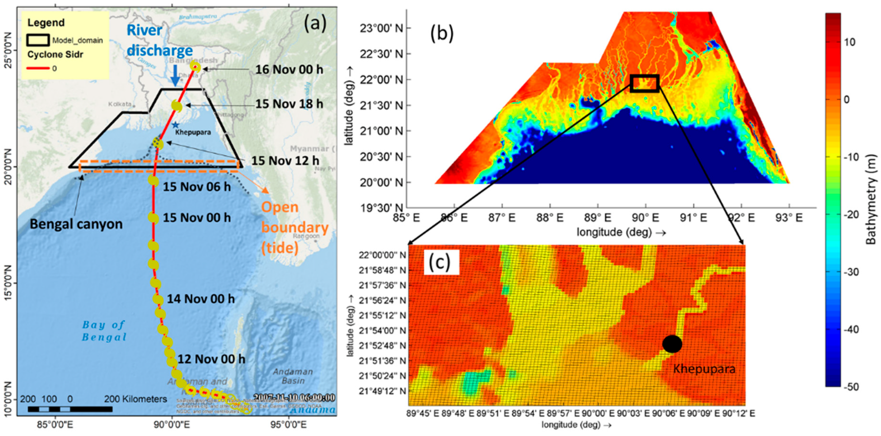
2.1. Cyclone Sidr

Cyclone Sidr made landfall near Khepupara at 1500 UTC on 15 November 2007. Cyclone Sidr was categorized as a ‘Category 5’ cyclone, with a minimum central pressure of 944 hPa and a maximum 1-min sustained wind speed of 260 km hr⁻¹. The surge height exceeded 7.5 m, and approximately 10,000 fatalities were reported [59]. The different cyclonic parameters of Cyclone Sidr are available from the best track archives of the Joint Typhoon Warning Centre (JTWC).

2.2. Study Area

Bangladesh is one of the world’s disaster-prone countries with 97.7 percent of the total population exposed to multiple hazards, including cyclones [60]. Devastating cyclones that form in the Bay of Bengal cause 80–90% of the global loss from cyclones. More than 30 percent of the total population lives in the coastal area making the GBMD vulnerable to cyclone-induced storm surges. The presence of a continental shelf, a deep submerged canyon 100 km from the coast, and the funnel-shaped geography results in the amplification of surge height in the GBMD. In addition, the coastal land area lies between 1 to 3 m above mean sea level.

The GBMD is an active delta that conveys 1 billion tons of sediment to the Bay of Bengal from the upper catchment area. Due to dynamic river morphology in the central GBMD, the river bathymetry changes rapidly, particularly in the mouth of the Lower Meghna river. The presence of extensive shoals, shallow lands, and islands in the lower Meghna river’s estuary mouth causes complex hydrodynamic features compared to other estuary systems [61]. Moreover, the Lower Meghna River, the third-largest source of freshwater discharge to the ocean, conveys 80% of the combined freshwater discharge of the Ganges, Brahmaputra, and Meghna rivers from the upper catchment area to the Bay of Bengal. The Lower Meghna River has significant seasonal variations in river discharge up to 100,000 m³ s⁻¹. Other rivers located in the western GBMD, including the Bishkhali and Baleswar, are tide-dominated and convey a negligible amount (<3000 m³ s⁻¹) of freshwater compared to the central GBMD. There are a few hilly rivers located in the eastern part of the GBMD, which convey freshwater during flash flood events during the monsoon season. Tides in the GBMD are semi-diurnal with a mean tidal range varying from 3 to 6 m along the coast. Tides can propagate over 200 km inland and have strong seasonal variations with the seasonal river discharge variations. Details of variations in river discharge and tides are discussed in Elahi et al. [62]. To help mitigate the coastal flooding from storm surge events, 123 earthen embankments were constructed across the GBMD. These structural interventions caused changes in flooding patterns in the coastal area by reducing natural floodplain area, and increasing river-bed siltation [63].

April to May (early summer) and October to November (late rainy season) are the two main seasons when most of the severe cyclones impact the GBMD. Cyclone Sidr made landfall on the Bangladesh coast on 15 November 2007 during the late rainy season. According to previous studies [46,49], the river discharge from the Ganges, Brahmaputra, and Meghna rivers are 15,000 m³ s⁻¹, 25,000 m³ s⁻¹, and 850 m³ s⁻¹ during Cyclone Sidr, respectively. Cyclone Sidr is one of the most well-documented cyclone events to have occurred on the Bangladesh coast. Case studies have investigated the socio-economic impacts [64] and physical storm surge processes [49] during Cyclone Sidr. Hence, the current study focuses on wave–current interactions during the Cyclone Sidr surge event. The shallow continental shelf, high tidal range variations, the triangular shape of geography, and low-lying land elevation make the GBMD a perfect laboratory to study the wave–current interactions during a cyclone-induced storm surge event.

2.3. Field Data

Compromises are often made between parameters in storm surge models used for research [49] to reproduce the maximum water levels at a single tide gauge. For example, the model may reproduce the maximum water level without considering waves by overestimating wind surge using an artificial increase in maximum wind speed or the radius of maximum wind. Similarly, errors in other factors such as bathymetry, bottom friction, or drag coefficient can offset each other to some extent so that water levels can be correctly reproduced at one location, even when the model does not accurately reproduce the physical processes [49]. For this study, it is important to ensure that the model properly represents physical processes and accurately represents the water levels during the storm surge event. To do this, the model needs to be validated against a representative set of water level, wind, and wave observations at different locations.

Water level observations during cyclonic events in the GBMD are rare. There are several tide gauge stations located in the coastal areas. These stations are maintained by two different governmental institutions: the Bangladesh Water Development Board (BWDB); and the Bangladesh Inland Water Transport Authority (BIWTA). The float gauges used in these stations are located in remote areas of the coastal zone and the benchmarking and datum checks are not updated regularly. Gaps in the observations and reduced sampling rates occur in the water level data set because of tidal gauge malfunctions [65]. There are several limitations regarding water level observations such as the relatively short supply of automatic tide gauges, poor documentation, and displacement of tide gauges sometimes by floods or due to maintenance, which makes it difficult to validate models consistently in the GBMD [49]. In addition, tide gauges are often located in rivers that are not resolved by models. Consequently, the validation process in studies often consists of checking that the order of magnitude of the maximum water level is reproduced in the grid wet node that is closest—but sometimes 10 km away or more—from the actual tide location [49]. Cyclone Sidr made landfall at the mouth of the Bishkhali river, which is a tidal river with a very low freshwater outflow (<3000 m³ s⁻¹) compared to the Lower Meghna river (<100,000 m³ s⁻¹). The water level variations during Cyclone Sidr are available at Hironpoint, Khepupara, and Coxsbazar from the BIWTA. Further details of monitoring stations are discussed in Section 4.1. In the current study, the model water levels are compared at these three stations.

Finally, to increase the amount of validation data for the model, the significant wave height and atmospheric surface wind data from the European Center for Medium-range Weather Forecasting (ECMWF) ERA5 reanalysis dataset [66] is used to validate the model wave heights. The ERA5 dataset is a global atmospheric and ocean surface 0.5° × 0.5° grid resolution dataset available every hour and provides coverage of the deep ocean area of the study region.

3. Methodology

A numerical model based on Delft3D with the Delft3D-Wave model is used to simulate the cyclone-induced storm surge event in the GBMD. The model is calibrated and validated based on available data during Cyclone Sidr. Several idealized scenarios are then designed and analyzed to investigate the influence of wave setup and wave–current interaction on the simulated storm surge height. Details of the model setup and processes are discussed in the following sections.

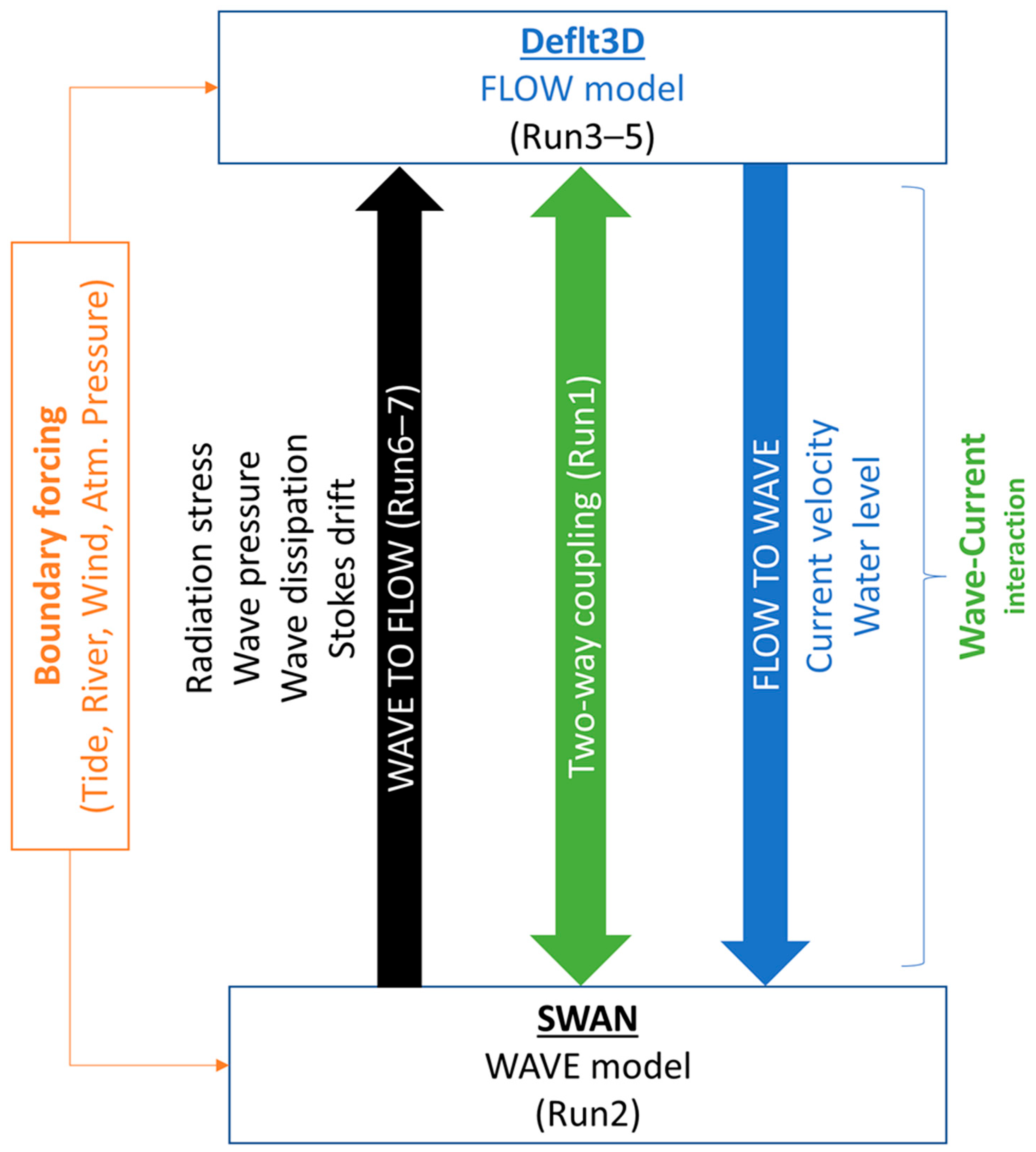
3.1. Numerical Model Delft3D

The standard Delft3D package [67] has been widely applied for modeling physical processes (e.g., hydrodynamics and sediment transport) in coastal oceans, estuaries, and lakes [68]. In the present study, the standard Delft3D package is applied to simulate the interactions between wave and current in the GBMD. Delft3D-FLOW (referred to as the FLOW model for the rest of the paper) solves the unsteady shallow-water equations using a finite difference scheme under Boussinesq and shallow water assumptions. Further details about Delft3D-FLOW can be found in Lesser et al. [67] and Deltares [68]. Delft3D-WAVE (referred to as WAVE model through the rest of the paper) is a modified version of the third-generation SWAN model [55,69], which performs well during the evolution of random, short-crested wind-generated waves in the coastal environment (Deltares, 2018). A brief description of the Delft3D-WAVE from Deltares [70] is given below.

3.1.1. Wave Setup

The presence of wave includes radiation stress term in the momentum balance equation. Hence, the hydrostatic pressure gradient is modified to balance the wave forcing based on the following vertical integrated momentum balance equation in the 1D (cross-shore) case [14,16]. Wave setup results from a balance between the wave force (gradient of the wave radiation stress) and the hydrodynamic pressure gradient. Note that wave setup is calculated in the FLOW model.

$$\frac{d{S}_{xx}}{dx}+\rho gH\frac{d\eta }{dx}=0$$

(1)

where H = d + η denotes the total water depth and η represents the mean surface elevation including the wave setup; S is the radiation stress tensor:

$$\begin{gathered} S_{xx}=\rho g\int \left(nco{s}^2\theta +n-\frac{1}{2}\right)Ed\sigma d\theta \\ {S}_{xy}=S_{yx}=\rho g\int nsin\theta cos\theta Ed\sigma d\theta \\ {S}_{yy}=\rho g\int \left(nsi{n}^2\theta +n-\frac{1}{2}\right)Ed\sigma d\theta \end{gathered}$$

(2)

and n = c_gk/ω is the ratio of group velocity over phase velocity; E is the wave energy.

In the present study, the model setup uses 2d radiation stress parameterization. However, in the 3d model implementation in Delft3d, the bed shear stress and wind shear stress are considered as the bed- and surface boundary conditions. The details formulation can be found in Cats [71] (see equation 3.8–3.11 in Cats, 2014). Moreover, in wave force calculation in the 3d model, the force due to radiation stress gradient is applied only at the surface layer of the vertical grid. The Delft3D-FLOW uses the dissipation rate (the total wave energy dissipation estimated from the SWAN) to model the excess flux of momentum (see equation 3.39–3.40 in Cats [71]). For further details of forcing by radiation stress gradient can be found in section 9.7.1 in the Flow User Manual Delft3d [68].

3.1.2. Wave-Current Interactions and Coupling Procedures

Delft3d considers five physical processes in computations of wave–current interactions [68]. These are (1) radiation stress gradients [14], which are considered in the flow momentum equations; (2) enhance bed shear stress [72]; (3) induced vertical mixing and turbulence [67]; (4) streaming, which is a wave-induced current in the wave boundary layer directed in the wave propagation direction [73] and (5) Stokes drift and mass flux, which is accounted for via a Generalised Lagrangian Mean (GLM) approach [74]. Wave energy dissipation can transfer momentum to the eulerian flow via radiation stress gradient. The wave energy dissipation rate in SWAN is estimated internally as the sum of energy dissipation related to depth-induced breaking, whitecapping, and bottom friction per unit of time. The energy dissipation related to wave breaking is estimated by the formulation of Battjes & Janssen [75]. Detail method of the wave–current interactions in Delft3d can be found in the Flow User Manual Delft3D (See section 9.7, Page 220 in Deltares, [68]).

Delft3d module offers different types of wave computations such as a standalone wave computation using SWAN, an offline coupling of WAVE with Delft3d-FLOW, and an online coupling of WAVE with Delft3d-FLOW. In the case of the offline coupling or the online coupling between the FLOW and WAVE modules of Delft3d, data is exchanged using a communication file (com-file), which contains the most recent data of the flow and wave computations. Coupling between the WAVE and FLOW models can be one-way or two-way, which means the interactions (i.e., information transfer) between the two models occur unidirectionally and bidirectionally, respectively (Figure 1). Further details of the coupling procedure can be found in the Delft3d wave user manual [70].

3.2. Model Setup and Boundary Forcings

The model river and estuary bathymetry are prepared by using measured cross-sections collected from 2007 to 2014 within the ESPA-delta (Assessing health, livelihoods, ecosystem services and poverty alleviation in populous deltas) project of the Bangladesh University of Engineering and Technology (BUET). The inland ground elevation data is specified from the FINNMAP (a Finland-based private organization) Land Survey 1991, National Digital Elevation Model (DEM) from Floodplain Action Plan-19 (FAP19), which were collected through aerial photographic surveys and field measurements by the Centre for Environmental and Geographic Information Services (CEGIS), Bangladesh. The ocean bathymetry is specified using open-access data from the General Bathymetric Chart of the Oceans (GEBCO, http://www.gebco.net/) (27 September 2018). As the model bathymetry is prepared based on the field measurements on different periods, it may affect the model performance to capture a realistic scenario of cyclone Sidr in 2007. The present study assumes no significant differences in bathymetry over 2007–2014.

The model is setup to simulate storm surge events in the GBMD. In this study, a three-dimensional version of Delft3D is used to set up the barotropic model for the GBMD. Two-way coupling of the FLOW and WAVE model is applied to the establishment of the model setup. The model setup is computed on a boundary-fitted curvilinear grid of 200–1320 m resolution with ten sigma layers in a vertical direction. The combined time-varying river discharge of the Ganges–Brahmaputra–Meghna river is applied at the upstream boundary condition following Krien et al., [49]. Astronomical constituents (K1, O1, P1, Q1, M2, S2, N2, K2, M4, MS4, MN4, MSF) for the water level at downstream locations are generated by applying the TPXO 7.2 Global Inverse Tide Model [76]. Details of the model domain including the location of open boundary forcings and model bathymetry are presented in Figure A1 in Appendix A.

The cyclonic wind and pressure field are generated from the JTWC cyclone best track for Cyclone Sidr (2007) over the computational grid by using the Delft-Dashboard module (DDB) [77]. The DDB calculates wind and pressure fields on a moving circular spider web grid for the given track information data, based on the Wind Enhancement Scheme (WES) following Holland [78]. The Holland profile is a smooth analytic profile of wind and pressure extending from the cyclone center to the outer radius and is shaped by cyclone parameters including maximum wind intensity, the radius of maximum wind, and minimum pressure from the JTWC best track archive. The details of cyclonic wind and pressure fields incorporation as boundary forcings are described in Appendix A.2. The generated cyclonic wind and pressure fields are included as the spatial and temporal varying surface boundary conditions for the FLOW and WAVE models. The WAVE model is applied with 36 directions and 24 frequency bins, with the cut-off frequencies being 0.04 and 1 Hz.

The model simulation period is 10–16 November 2007. The model was calibrated by applying different combinations of Manning’s coefficient and then comparing modeled and observed water levels at Hironpoint, Khepupara, and Chittagong stations for Cyclone Sidr (2007). An increasing roughness parameter from 0.00025 (sea) to 0.05 (upper estuary) provided the best reproduction of observations. Other parameterizations are specified in

Table 1. Model parameterization.

Delft3d FLOW
Parameters	Model	Coefficients
Bottom roughness	Manning	0.00025–0.05 (sea to land)
Stress formulation	Fredsoe, 1984
Background horizontal viscosity/diffusivity	-	1 m2 s−1
Background vertical viscosity/diffusivity		0.1 m2 s−1
Model for 3D turbulence	k-Epsilon
Wind drag coefficients		0.001 for U10 = 0 m s−1 0.003 for U10 = 30 m s−1
Time step		0.5 min
SWAN
Generation mode for physics	3-rd generation
Depth-induced breaking	B&J model (Battjes and Janssen, 1978)	Alpha = 1, Gamma = 0.73
Non-linear triad interaction	-	Alpha = 0.1, Beta = 2.2
Bottom friction	JONSWAP	Coef. = 0.08 m2 s−3
Diffraction	-	Smoothing coef. = 0.2 Smoothing steps = 5 Adapt propagation = Yes
Other processes activated in SWAN
Wind growth	Yes
Whitecapping	Yes (following Komen et al., 1984)
Wave propagation in spectral space	Refraction and Frequency shift are activated

. A full validation analysis is detailed in Section 4.1. The different tidal component variations in the GBMD for different hydrodynamic years were already investigated by Elahi et al. [62], and the FLOW model setup shows good accuracy in producing the tidal forcing in the study area. The same tide boundary forcings are applied in the current study. Hence, we did not include the tidal variation analysis in the current study.

3.3. Description of Scenarios

Scenarios to investigate different physical processes related to cyclone-induced storm surge events are designed by modifying the model setup and boundary forcings. Six sensitivity scenarios are designed to address the role of different factors, including wave–current interactions, in the generation of storm surge height during a cyclonic event. To reduce the computational time, the sensitivity simulations (except the control run, Run1) are run for just the last four days of the Cyclone Sidr period (13–16 November 2007). The simulation period covers the time from two days prior to landfall until the cyclone dissipated at 0000 UTC on 16 November 2007.

Six scenarios including the control run are designed to assess the influence of wave–current interaction on storm surge height generation during Cyclone Sidr (

Table 2. Scenario details to investigate the influence of wave–current interaction in cyclone-induced storm surge height.

Experiment Designed to Study Wave Influence
Run Name	Simulation	Description	Coupling Method
Run1	Control run	FLOW and WAVE simulation	Two-way
Run2	Wave only	WAVE simulation	No coupling
Run3	Current only (tide)	FLOW simulation with only tide forcing	No coupling
Run4	Current only (Wind)	FLOW simulation with only wind forcing	No coupling
Run5	Current only (Tide and Wind)	FLOW simulation with tide and wind forcing	No coupling
Run6	Current only (Tide and Wind with Wave)	FLOW simulation using only radiation stress from Run2	One-way (WAVE to FLOW)
Run7	Current only (Ignoring Tide and Wind, only wave-driven current)	FLOW simulation using only radiation stress from Run2	One-way (WAVE to FLOW)

). A two-way coupled model considering all the boundary forcings including tide, wind, atmospheric pressure, wave, and river discharge is calibrated and validated, to produce the most realistic recreation of Cyclone Sidr (Run1). Run2, Run3, and Run4 are uncoupled and consider only wave, only tide, and only wind, respectively. Finally, Run5, which considers tide and wind without coupling, is used to evaluate the combined influence of tide and wind in the generation of cyclone-induced storm surge height (Table 2). By comparing Run1 and Run5, the model wave setup and influence of wave–current interaction are examined. Similar modeling approaches have also been applied in Bohai Bay, China, to study wave–current interactions during extreme weather conditions by Song et al. [29].

4. Result and Discussions

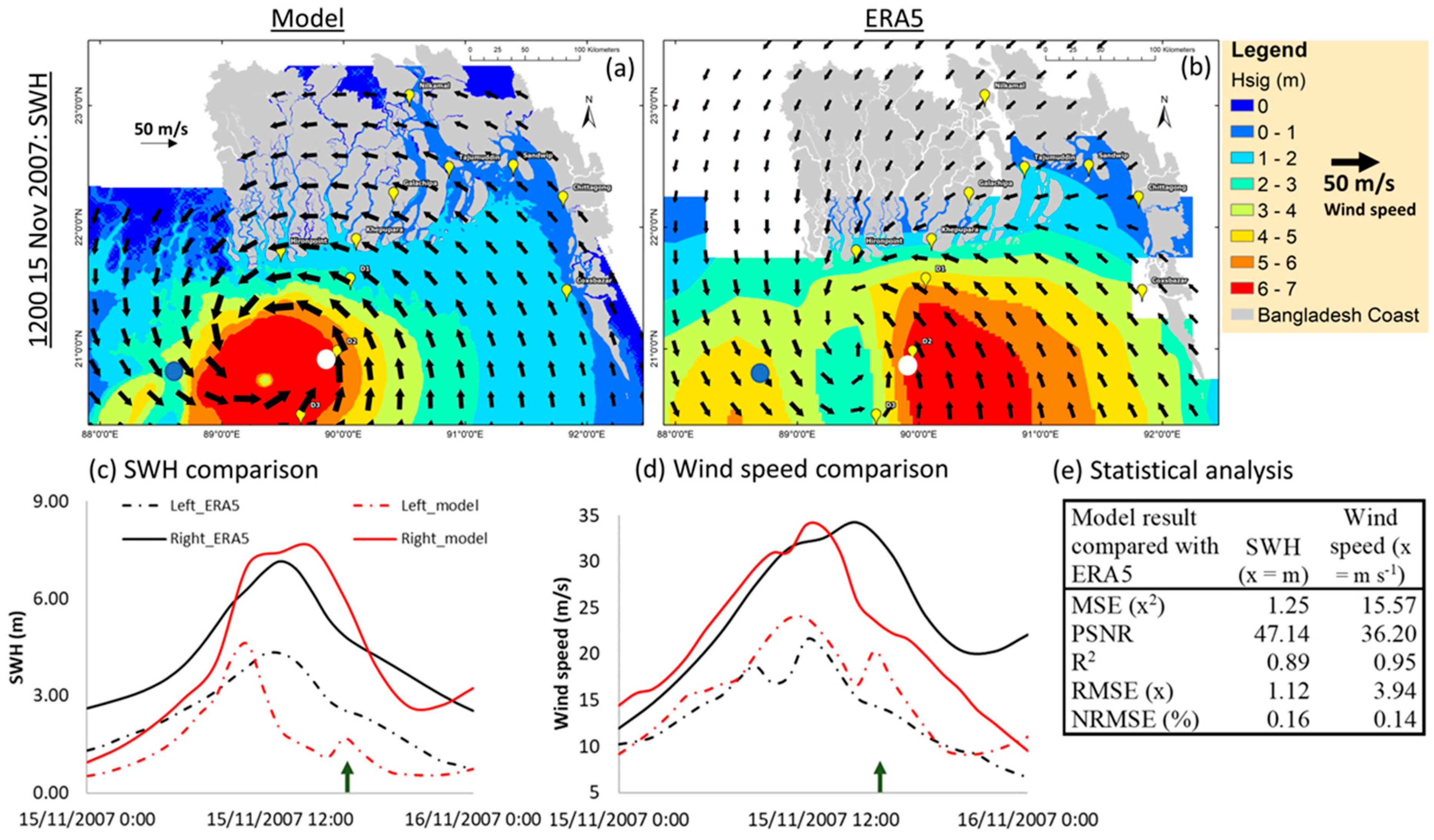
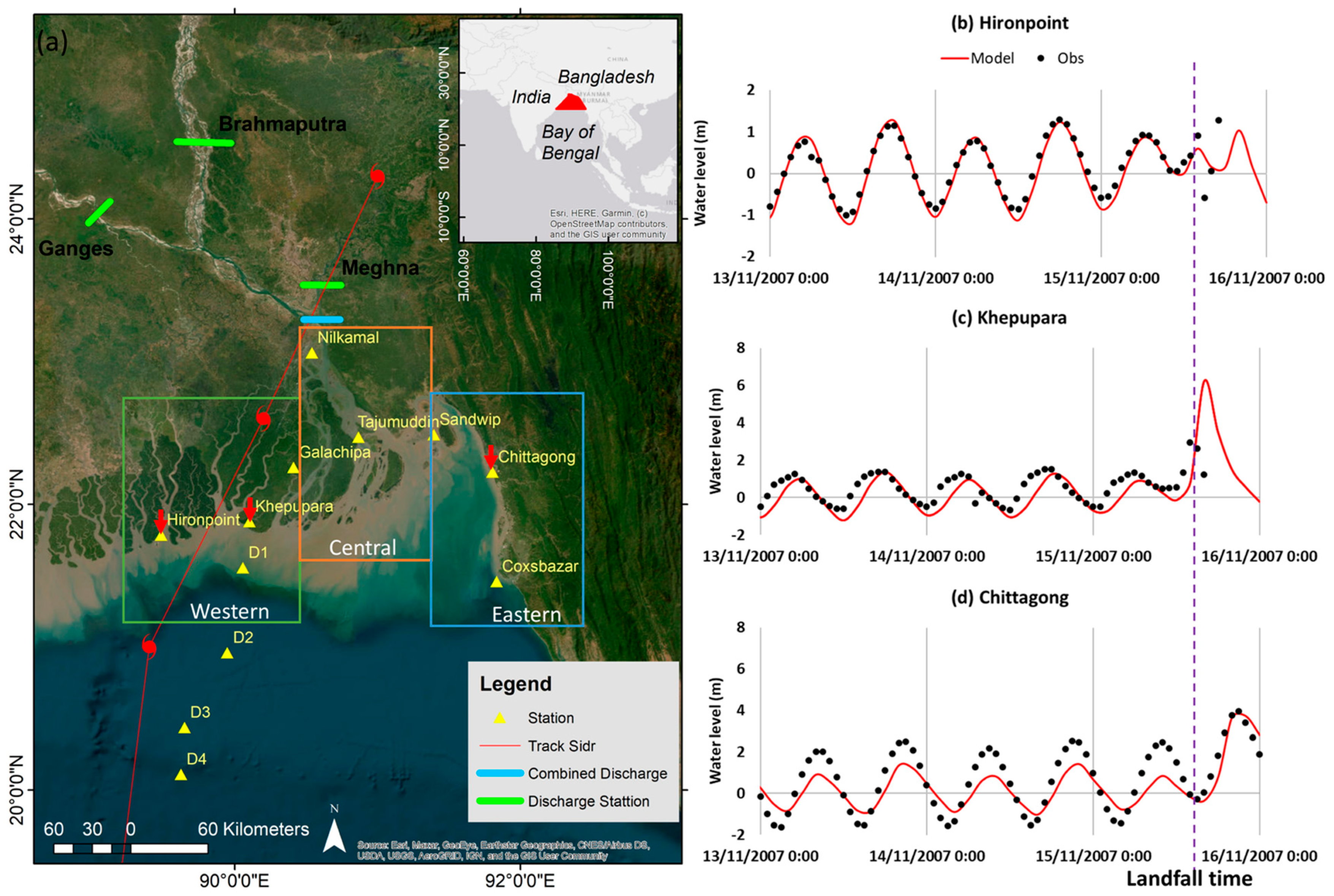
4.1. Model Validation

The model simulated water level (from Run1) variations during Cyclone Sidr are compared with observations at Hironpoint (Figure 2b), Khepupara (Figure 2c), and Chittagong (Figure 2d) (

Table 3. Statistical analysis of model water level compared with observations for cyclone Sidr.

(Water Level)	Hironpoint	Khepupara	Chittagong
MSE: Mean squared error (m2)	0.08	0.46	0.74
PSNR: Peak signal-to-noise ratio	59.37	51.50	49.41
R sq. value:	0.84	0.44	0.71
RMSE: Root mean square deviation (m):	0.27	0.68	0.86
NRMSE: Normalized Root-mean-square error (%)	0.12	0.19	0.15

). The model reproduces the storm surge signals at all these three stations reasonably well with better performance at Hironpoint (R² = 0.84) and Chittagong (R² = 0.71) compared to Khepupara (R² = 0.44), perhaps because Khepupara stopped working during the landfall period [79]. After the cyclone made landfall, the gauge stations stopped working, and the peak water levels at Hironpoint and Khepupara were missed. At Chittagong, the model water level was consistently underestimated by approximately 1.5 m for the preceding four days prior to landfall. This error could be contributed by errors in the bathymetry since the Chittagong estuary lacks field measurements and the bathymetry is based on the GEBCO dataset. In contrast, the maximum model high water level during the cyclone event matches the observations at Chittagong, indicating that the model successfully captures the storm surge peak signal. The model results demonstrate that it can capture the phase of maximum and minimum water level observations along with the storm surge peak.

There are few available observations of wind speed and wave height in the GBMD delta and so, the model results are compared with the ERA5 reanalysis dataset [80]. The ERA5 ocean data does not resolve the estuary mouth regions of the GBMD and a point-by-point comparison of model significant wave height (SWH) and model wind speed with the ERA5 data is not possible because of the very different model grid resolutions. Therefore, the model data are compared with the ERA5 data at two locations, one on the right side and one on the left side of the cyclone’s eye near the radius of maximum winds. Figure 2a,b shows the model and the ERA5 SWH at 1200 UTC on 15 November 2007, three hours earlier than Cyclone Sidr’s landfall time. The results show that the model can reproduce the spatial variations of SWH variations due to cyclonic conditions in the study area. The time series of wind speed and SWH are compared at two points: one is on the right side (90.94° E 20.76° N) and the other is on the left side (88.56° E 20.80° N) of the cyclone eye, and presented in Figure 3a,b. Figure 3c–e shows that the model can reproduce the trend of temporal variations of SWH (R² = 0.89) and wind speed (R² = 0.95) of the ERA5. The peak values are similar although there are finer temporal variations in the model SWH (RMSE = 1.12 m) and wind speed (RMSE = 3.94 m s⁻¹) compared with the ERA5 likely due to the better resolved spatial features in the wind and SWH near the radius of maximum winds in the much finer model grid. The statistical analysis at these two points (Figure 3e) demonstrates that the model can reasonably reproduce SWH and wind speed in the BoB during the cyclone event.

Many studies have investigated the storm surge event during Cyclone Sidr. Among them, Deb and Ferreira [39] and Krien et al. [49] consider the wave–current interaction in their study, whereas, other studies neglect the wave–current interaction [46]. Deb and Ferreira [39] focus on storm surge height variations in the Bangladesh coastal area for the first time by considering wave influence and demonstrating that waves can influence surge height. However, the study is restricted to the exposed coastal area due to a lack of good bathymetry and a relatively coarse grid resolution (e.g., 900 m). Moreover, Deb and Ferreira [39] do not discuss how the wave–current interaction influences wave height. A comparison of our model results with Deb and Ferreira [39] and Lewis et al. [46] is provided in

Table 4. Comparison of model outcomes with high water levels and max. significant wave height extracted from recent studies on Cyclone Sidr.

Locations	Chittagong	Coxsbazar	Sandwip	Khepu Para	Galachipa	Hironpoint	R2	RMSE (m)
Lat	22.19	21.46	22.48	21.88	22.03	21.81
Long	91.81	91.92	91.55	90.10	90.34	89.49
High water level during cyclone Sidr (m)
This study	4.8	2.4	6.1	6.5	5.4	1.2
Deb and Ferreira, 2016	3	2.0	4.5	5.9	6.5	2.5	0.92	1.23
Lewis et al., 2013	3.2	2.0	3.4	5.5	6.1	2.5	0.87	1.48
Maximum significant wave height during cyclone Sidr (m)
This study	1.7	1.6	2.2	2.9	1.6	3.1
Deb and Ferreira, 2016	3.2	1.8	3.1	2.1	3	3	0.87	0.97

and demonstrates that the model can reproduce reasonable high-water levels and maximum SWH during Cyclone Sidr compared with other published modeling studies. The water level has a higher RMSE for the Lewis et al. [46] study compared with the Deb and Ferreira [39] study. Since Lewis et al. [46] do not consider the wave–current interaction, this is reasonable. The evolution of the high-water level (R² = 0.92) and maximum significant wave height (R² = 0.87) demonstrate good agreement with Deb and Ferreira [39]. While the model maximum SWH is underestimated by 1.5 m and 1.4 m compared to Deb and Ferreira [39] at Chittagong and Galachipa, respectively. Galachipa is located between two earthen embankments and is further inland compared to other stations. Since Deb and Ferreira [39] do not consider embankment heights in their study, the difference in the maximum SWH likely has resulted from the improved bathymetry and finer grid resolution in this current study. Overall, the model in this study reproduces the storm surge event in the GBMD reasonably well.

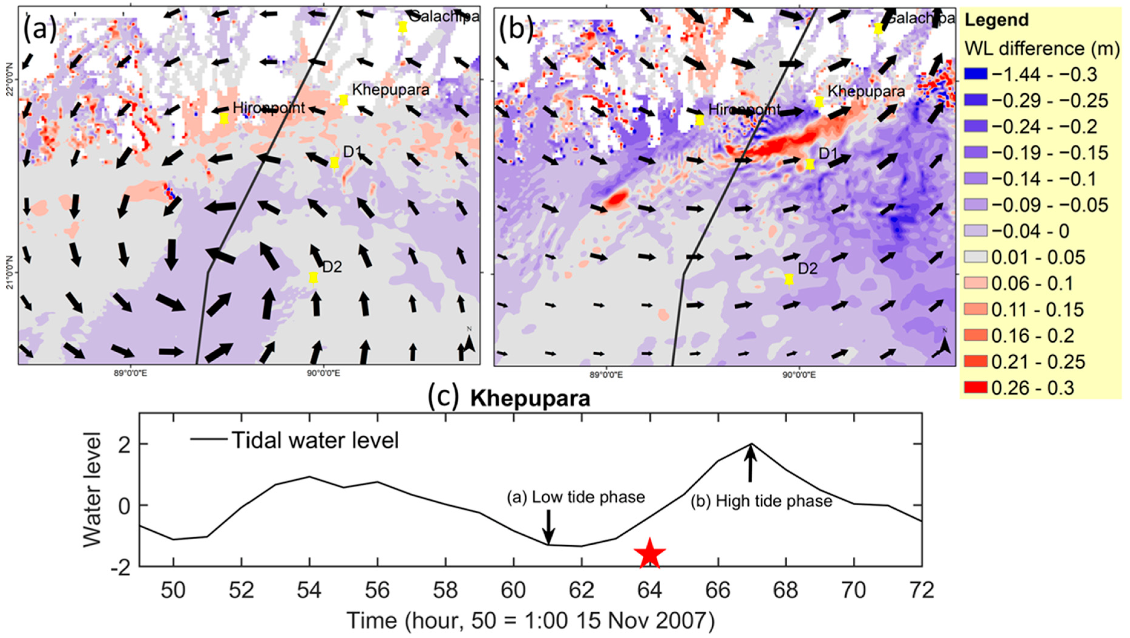
4.2. Surface Water Elevation Variations

Cyclone Sidr made landfall at Khepupara on the Bangladesh coast in the western GBMD at 1500 UTC on 15 November 2007. The cyclone tracked slightly east of the north and passed close to several stations including Khepupara, Galachipa, D1, and Hironpoint (Figure 4), which recorded maximum winds of ~50 m s⁻¹.

As the cyclone approached the coast it produced storm surges across the GBMD with the central GBMD (Figure 4a) experiencing up to 7 m of high-water level during the landfall event [39]. Figure 4 shows the evolution of the model surface water elevation for the control run simulation (Run1 in Table 2) at 3-h intervals on 15 November 2007. At 1200 UTC, while the center of Cyclone Sidr was still well offshore (Figure 4a), the western (green box in Figure 2a) and central (orange box in Figure 2a) GBMD coastline was under the influence of the outer easterly wind field north of the cyclone center. The eastern GBMD (blue box in Figure 2a) was located east of the cyclone center and the outer-core winds extending onto this coastline were southerly. Because of the funnel-shaped geometry of the GBMD coastline, the surface water elevation initially increased on the eastern edge of the estuary mouth in the eastern GBMD driven by the southerly outer-core wind field east of the cyclone center.

By 1500 UTC as the cyclone approached land, the strong inner-core wind field began to directly affect the coast in the western and central GBMD (Figure 4b). The strong inner-core southerlies north and east of the cyclone center drove increased water elevations in the western GBMD with a maximum of 7.2 m observed at Khepupara (middle red arrow in Figure 4a). As the cyclone continued to move inland over the course of the next few hours (Figure 4c,d), the strong wind field moved inland over the central GBMD, and the high water levels were driven inland along the numerous rivers and narrow channels in the delta region with anomalous water levels of more than 4 m (Figure 3d and Figure 4c). By 2100 UTC the high-water levels had spread inland up the Meghna River and east to the eastern GBMD.

Throughout the period as the cyclone approached, made landfall, and then continued to move inland, the main storm surge shifted across the delta region with initial high-water levels in the eastern GBMD while Cyclone Sidr was still well offshore and then shifting to the landfall region in the western GBMD as Cyclone Sidr made landfall and then extending east to the central, and finally back to the eastern GBMD. The main driving forces for the increased water levels were the cyclonic winds that were directed perpendicular to the coast (e.g., Figure 4b–d). Thus, the eastern GBMD was affected earlier than the other regions because the outer core winds ahead of the cyclone center were directed perpendicular to that coastline ahead of the arrival of the cyclone’s inner core. Even after the most intense inner-core winds had moved inland and dissipated, the strong outer-core storm-force winds (~24 m s⁻¹) still continued to force storm surges into the central and eastern GBMD (Figure 4d).

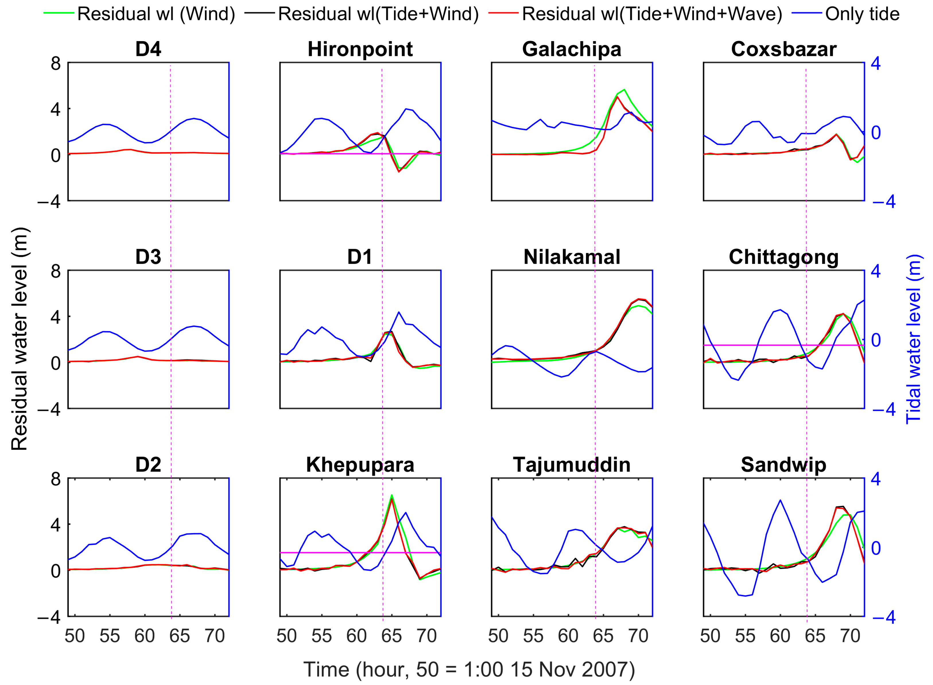
4.3. Role of Tide, Wind, and Waves in the Storm Surge Height

The magnitude variations of the surface elevation depend not only on the wind but also on the tides and wind-driven waves. Although the strong surface wind is the dominant factor in generating the cyclone-induced storm surge height, other factors including the tidal phase and wave–current interactions can also contribute further to the surge height. The time-varying atmospheric pressure drop is applied as the boundary condition along with the wind whenever the wind is considered in the simulation. By analyzing the sensitivity of the water level to changes in cyclone pressure, we found that the contribution related to the pressure in the total water level (isostatic response) is negligible compared to the wind setup (<10% of the wind setup). Therefore, the contribution of the isostatic response of the sea level to surface elevation variation is ignored in the rest of the discussion. However, to study the influence of the tide, cyclonic wind, and wave on the storm surge height, the model is applied to four different experiments: (a) only tide (Run3 in Table 2, no coupling), (b) only wind (Run4), (c) tide and wind (Run5) and (d) considering tide, wind and wave together using two-way coupling (Run1). The time series of residual water level variations at different stations across the GBMD are presented in Figure 5. The residual water level is computed by subtracting the tidal water level from the total water level.

The total water level of the storm surge height is a combined result of tide, wind, pressure, and wave influence on the water level. Figure 5 demonstrates that the landfall time (64 h in Figure 5) occurs during different tidal phases across the GBMD. Hussain and Tajima [59] discussed the tidal characteristics in the eastern part of the GBMD. They observed an approximately 2-h tidal phase difference between the incoming tides at the western end and incoming tides at the eastern end. As a result, the tide propagates in a northeast direction toward the Bangladesh coast in an oblique manner and simultaneously reaches the coast of Hironpoint (station located on the left side of the cyclone track in Figure 2a) and Coxsbazar (Figure 2a), which is also mentioned by Hussain and Tajima [59]. Thus, during the landfall time, the tidal phases are in flood tide at the western GBMD (Khepupara) and ebb tide in the central GBMD (Tajumuddin). Due to the lower water level during the ebb tide phase in the central GBMD, Tajumuddin and Sandwip stations show relatively lower surge heights compared to the stations in the flood tide phase (e.g., Khepupara).

During a cyclone-induced storm surge event, the wind is typically the dominant factor producing the storm surge. By comparing the “only wind” (Run4) scenario with the “wind + tide” (Run5) and the “wind + tide + wave” (Run1) scenarios, it can be seen that the wind setup (described as wind-driven water level) explains the total water level at all stations except Khepupara, Galachipa, Nilkamal and Sandwip (Figure 5). The inconsistencies in residual water levels among the “only wind” scenario and other scenarios at these stations demonstrate that the wind setup is inversely proportional to total water depth, which is affected by tides. For example, the residual water level differences among the “only wind” (Run4) and “wind + tide” (Run5) result from the wind-tide interaction, which causes the wind setup to be decreased at high tide (e.g., 0.05–0.04 m Galachipa) and increased at low tide (e.g., 0.72–0.53 m at Sandwip). Furthermore, the stations located offshore are less affected by wind setup. This is why D2–D4 (>100 m) have a lower maximum storm surge height compared to the station located closer to the coast (e.g., D1 < 15 m) even though all these stations are close to the cyclone path.

During a cyclonic event, the water level variability at a location relative to the cyclone center is affected by the speed and direction of the winds at the station, as well as how the cyclone changes over time as it passes by. Hence, the timing of the peak water level due to the wind also varies from station to station. For example, Chittagong and Coxsbazar are located approximately 300 km from the landfall location. Though these two stations are relatively less affected by the strong cyclonic wind, they exhibit peaks in the water levels 4 h after the landfall time (Figure 5). Results show that the peak water levels at Chittagong and Coxsbazar are 2 m and 1.8 m higher, respectively, when compared to the “only tide” (Run3 in Table 2) scenario. This indicates that the cyclonic wind exerts only a weak influence on the water levels at these stations. Khepupara and Galachipa experience higher residual water levels compared to other stations. Both stations are located on the right side and close to the cyclone track in the strongest wind region. Hironpoint is also located close to the cyclone track, but on the left side of the cyclone track (Figure 2a). The wind direction on the right side of the cyclone eye is southerly, and the left side of the cyclone eye is northerly during the approach of, and at landfall. Therefore, wind setdown reduces the water level by up to 1.5 m at Hironpoint compared with the tidal water level during landfall regardless of whether waves are included in the simulation or not. All the other stations are located on the right of the track and are embedded in the generally southerly cyclonic flow. For these stations, there are significantly higher residual water levels compared with the only tide-driven experiment because of the wind setup.

When waves are also considered (Run1), there is no clear difference in the water levels compared to the wind and tide scenario (Run3), and this demonstrates the dominant role of wind setup in the cyclone-induced storm surge height. The tidal phase and amplitude also play a supporting role by modifying the combined influence of wind and tide on the storm surge height.

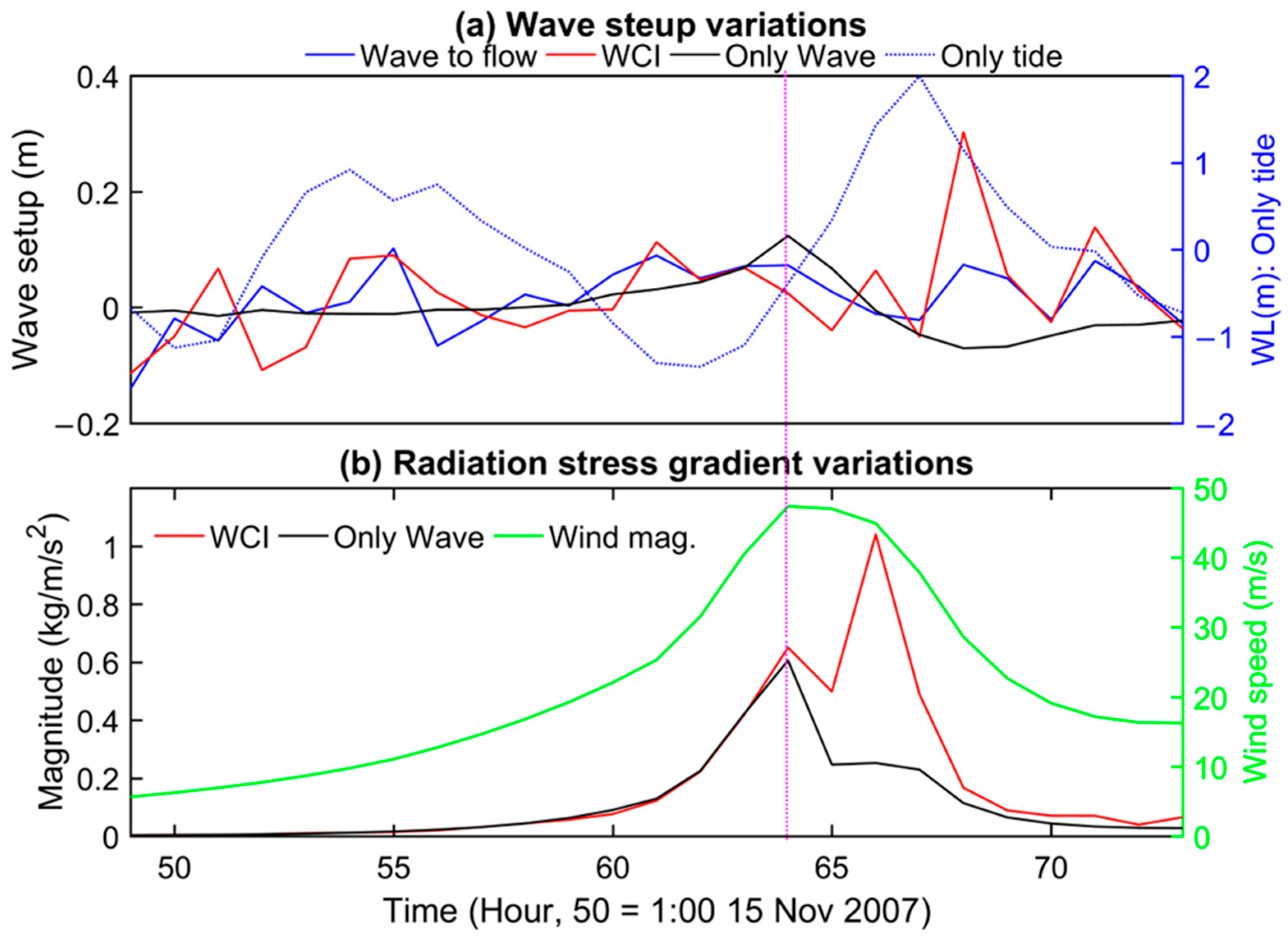
4.4. Role of Wave-Current Interaction in Wave Setup

Although the wind-driven wave contribution to the total water level is much less compared to the wind-driven water level there is an increment of over 0.25 m in the water level near Khepupara due to the wave coupling in Run1 (Figure 6). During low tide at 1200 UTC on 15 November, the wind is easterly, and the wind-driven waves produce a positive increment of up to 0.15 m of water level in the estuary and a maximum decrease of 0.10 m in the area close to the cyclone eye (Figure 6a). During high tide at 1800 UTC, which is 3 h after landfall, the wind has switched to westerly (Figure 6b). Furthermore, the higher water depth during the high tide contributes further to the wave setups as a result of larger waves produced by reduced bottom friction and bottom-induced wave breaking (e.g., Figure 6c). Hence, the wave coupling produces higher surface elevations near Khepupara compared with there being no wave coupling. Wave setdown also occurs in the mouth of the estuaries. This is because, after landfall, the wind blows from the land to the ocean near Khepupara. Therefore, the radiation stress gradient generated from the strong wind-driven wave moves water volume from the land toward the ocean, which causes wave setdown at the estuary mouth. Thus, waves have the potential to increase (decrease) the storm surge height up to 0.3 m through wave setup (setdown) near the landfall area in the GBMD during a cyclone-induced storm surge event. Figure 6 demonstrates that the wave influence on the water level varies with the cyclonic wind direction and tidal phase.

To further investigate the wave influence on water level variations during Cyclone Sidr, two one-way coupled FLOW simulations are designed: Run6 and Run7 in Table 2. Figure 7 shows the wave setup variations at Khepupara, where maximum surge height is observed during Cyclone Sidr. Khepupara is in the flood tide phase at the time of landfall, and water depth is below 10 m.

The wave setup for ‘Wave to flow’ (Run6 in Table 2), ‘WCI’ (Run1), and ‘OWC’ (Run7, only wave-driven current) are estimated by comparing the water level with Run5 (which considers tide + wind, Table 2). Figure 7 illustrates that during high tide wave–current interactions produce a higher wave setup at Khepupara relative to no wave–current interactions after landfall has occurred. In the ‘Wave to flow’ (Run6) scenario, the radiation stress gradient is unchanged due to the variation of currents and water levels in Equation (1). In the ‘OWC’ (Run7) scenario, the water level and current are only varied due to the radiation stress gradient as tides and winds are ignored in the FLOW model. It should be noted that the radiation stress gradients are the same in both ‘Wave to flow’ (Run6) and ‘OWC’ (Run7) scenarios. Hence, the differences between wave setups in both ‘Wave to flow’ and ‘OWC’ scenarios result from the influence of tides and winds on the total water depths and mean surface elevations in Equation (1).

The ‘WCI’ (Run1) scenario produces a maximum wave setup of 0.3 m at Khepupara, four hours after the landfall time (Figure 7a). The maximum wave setup of 0.07 m in the ‘OWC’ (Run7) scenario is observed during the landfall time and the maximum wave setdown by 0.07 m four hours after landfall at Khepupara. In the ‘Wave to flow’ (Run6), the combined influence of tides, winds, and waves results in a 7.5 m higher water depth (not shown in Figure 7) at Khepupara during landfall compared to the ‘Only Wave’ (Run2 in Table 2) scenario. According to Equation (1), if the radiation stress gradient is unchanged (in one-way coupling method, e.g., Wave to flow, Run6), then it is the high/low tide, causing larger/smaller water depth that will produce a smaller/larger increase in wave setup. Therefore, the ‘Wave to flow’ (Run6) scenario produces a higher wave setup (0.05 m) at 1200 UTC on 15 November (61-h in Figure 7) compared to the ‘OWC’ (Run7) scenario (low tide phase in Khepupara). At the landfall time, 1500 UTC 15 November (64-h in Figure 7), the increased water depth along with the unchanged radiation stress gradient causes 0.04 m lower wave-setup in the ‘Wave to flow’ compared to the ‘OWC’ scenario. Three hours after landfall (67-h in Figure 7), a maximum wave setdown of 0.02 m is observed in the ‘Only wave’ scenario due to the wave direction change.

Interestingly, the ‘WCI’ scenario changes from wave setdown to wave setup at 1900 UTC on 15 November (68-h in Figure 7) compared to the ‘OWC’ scenario at Khepupara. The ‘Wave to flow’ scenario also generates a wave setup of 0.07 m at 1900 UTC on 15 November (68-h in Figure 7). This indicates that the interaction between waves and currents can change the wave setdown to wave setup. As the radiation stress gradients are the same in both the ‘Wave to flow’ (Run6) and the ‘OWC’ (Run7) scenarios, the transformation of wave setdown to setup in ‘Wave to flow’ (Run6) must result from the increased water depth and mean surface elevations. In the ‘WCI’ (Run1) scenario, the radiation stress gradient is increased by approximately two times higher than in the other scenarios due to the increased wave energy dissipation (Figure 7b). Therefore, the ‘WCI’ (Run1) scenario generates a three times higher wave setup than the ‘Wave to flow’ (Run6) scenario. The reason behind increased wave energy dissipation at Khepupara will be discussed further in Part 2 of this paper [80].

5. Summary and Conclusions

Cyclone-induced storm surge events cause significant devastation in the GBMD. Due to the funnel’s geographical shape and the shallow coastal area (1–3 m above the mean sea level), storm surge heights are amplified and result in inundation in the GBMD. Although the GBMD is a tide-dominated delta, the strong winds during a cyclone event can produce substantial wave heights (e.g., approximately 3 m at Khepupara during Cyclone Sidr) at the coast. Several studies (e.g., [46]) have studied the cyclone-induced storm surge events in the GBMD, but the majority of studies neglected the wind-wave effects on the storm surge height except for Deb and Ferreira [39], and Krien et al. [49]. The major challenge to developing a numerical model for the region is the lack of wave-buoy data in the coastal area of the GBMD for calibration and validation. Continuous observed water level data are also scarce during cyclonic events because of the hazardous conditions that can cause damage to instruments. Therefore, most of the studies are based on the assumption that the wind wave has negligible impact on the storm surge height as the major portion of the wave dissipates far from the coastline due to the presence of a deep submerged canyon 80 km offshore that causes dissipation of wind-driven waves far from the coast. The current study illustrates that wind-driven waves and wave–current interactions are important considerations when reproducing cyclone-forced storm surges in the GBMD.

The findings of the current study show that the wind setup is the main contributor to generating cyclone-induced storm surge height during the cyclonic event. Based on non-linear interactions between wind, tide, and wind–wave, the storm surge height can be amplified/reduced along the coast. Wind setup (wind-driven water level) can explain the total water level except at Khepupara, Galachipa, Nilkamal, and Sandwip. The inconsistencies in residual water levels among the “only wind” scenario and other scenarios at these stations demonstrate that the wind setup is inversely proportional to total water depth, which is affected by tides. Moreover, considering the wind wave in simulation can increase the surface water level up to 0.3 m near the landfall location.

One major drawback of the study is that measured data on waves, water levels, and winds are limited in the study. Moreover, the model is not validated with the measured data on currents during Cyclone Sidr. To provide confidence in model quality assessment, we further conducted the cyclone-induced storm surge inundation comparison between the model and satellite image analysis of MODIS. As shown in Figure 8, reasonable matching of flooding between the model prediction and satellite image is a good confirmation of the model quality.

Finally, the dynamic characteristics of water level elevation and wave-induced setup and setdown along with the coastal areas, particularly during a storm surge event, have cumulative effects that depend on the mutual interaction between waves, currents, and tides [81]. Waves are modified by the presence of currents generated by the tide and surge. Breaking waves in the shallow region contribute to a radiation stress gradient that affects the resultant water level and circulation through wave-induced setup. Moreover, this may produce spurious wave setdown in the region (strongly influenced by current, e.g., Tajumuddin), when there is really wave setup occurring (figure not shown). This type of error can result in incorrect assumptions in the coastal management plan for cyclones. The wave setup and setdown are directly related to the generation and dissipation of wave energy. Therefore, the wave height variations and wave dissipations during Cyclone Sidr are further investigated in Part 2 of this paper [82] to understand the role of wave–current interaction during cyclonic events.

References

1. Yu, X.; Pan, W.; Zheng, X.; Zhou, S.; Tao, X. Effects of wave-current interaction on storm surge in the Taiwan Strait: Insights from Typhoon Morakot. Cont. Shelf Res. 2017, 146, 47–57. [Google Scholar] [CrossRef]
2. Roland, A.; Cucco, A.; Ferrarin, C.; Hsu, T.-W.W.; Liau, J.-M.M.; Ou, S.-H.H.; Umgiesser, G.; Zanke, U. On the development and verification of a 2-D coupled wave-current model on unstructured meshes. J. Mar. Syst. 2009, 78, S244–S254. [Google Scholar] [CrossRef]
3. Kim, S.Y.; Yasuda, T.; Mase, H. Wave set-up in the storm surge along open coasts during Typhoon Anita. Coast. Eng. 2010, 57, 631–642. [Google Scholar] [CrossRef]
4. Dietrich, J.C.; Zijlema, M.; Westerink, J.J.; Holthuijsen, L.H.; Dawson, C.; Luettich, R.A.; Jensen, R.E.; Smith, J.M.; Stelling, G.S.; Stone, G.W. Modeling hurricane waves and storm surge using integrally-coupled, scalable computations. Coast. Eng. 2011, 58, 45–65. [Google Scholar] [CrossRef]
5. Brown, J.M.; Bolaños, R.; Wolf, J. The depth-varying response of coastal circulation and water levels to 2D radiation stress when applied in a coupled wave–tide–surge modelling system during an extreme storm. Coast. Eng. 2013, 82, 102–113. [Google Scholar] [CrossRef]
6. Feng, X.; Yin, B.; Yang, D. Development of an unstructured-grid wave-current coupled model and its application. Ocean Model. 2016, 104, 213–225. [Google Scholar] [CrossRef]
7. Tolman, H.L. Wind Wave Propagation in Tidal Seas. Ph.D. Thesis, Technische Universiteit Delft, Delft, The Netherlands, 1990. [Google Scholar]
8. Zhang, W.-Z.; Shi, F.; Hong, H.-S.; Shang, S.-P.; Kirby, J.T. Tide-surge interaction intensified by the Taiwan Strait. J. Geophys. Res. Ocean. 2010, 115, 5762. [Google Scholar] [CrossRef]
9. Xie, L.; Wu, K.; Pietrafesa, L.; Zhang, C. A numerical study of wave-current interaction through surface and bottom stresses: Wind-driven circulation in the South Atlantic Bight under uniform winds. J. Geophys. Res. Ocean. 2001, 106, 16841–16855. [Google Scholar] [CrossRef]
10. Xie, L.; Pietrafesa, L.J.; Wu, K. A numerical study of wave-current interaction through surface and bottom stresses: Coastal ocean response to Hurricane Fran of 1996. J. Geophys. Res. Ocean. 2003, 108, 1–18. [Google Scholar] [CrossRef]
11. Mastenbroek, C.; Burgers, G.; Janssen, P.A.E.M. The Dynamical Coupling of a Wave Model and a Storm Surge Model through the Atmospheric Boundary Layer. J. Phys. Oceanogr. 1993, 23, 1856–1866. [Google Scholar] [CrossRef]
12. Signell, R.P.; Beardsley, R.C.; Graber, H.C.; Capotondi, A. Effect of wave-current interaction on wind-driven circulation in narrow, shallow embayments. J. Geophys. Res. Ocean. 1990, 95, 9671–9678. [Google Scholar] [CrossRef]
13. Davies, A.M.; Lawrence, J. Modeling the Effect of Wave? Current Interaction on the Three-Dimensional Wind-Driven Circulation of the Eastern Irish Sea. J. Phys. Oceanogr. 1995, 25, 29–45. [Google Scholar] [CrossRef]
14. Longuet-Higgins, M.S.; Stewart, R.W. Radiation stresses in water waves; a physical discussion, with applications. Deep Sea Res. Oceanogr. Abstr. 1964, 11, 529–562. [Google Scholar] [CrossRef]
15. Smith, J.A. Wave-current interactions in finite depth. J. Phys. Oceanogr. 2006, 36, 1403–1419. [Google Scholar] [CrossRef]
16. Longuet-Higgins, M.S.; Stewart, R.W. Radiation stress and mass transport in gravity waves, with application to ‘surf beats’. J. Fluid Mech. 1962, 13, 481–504. [Google Scholar] [CrossRef]
17. Gonazález, F.I. A Case Study of Wave–Current–Bathymetry Interactions at the Columbia River Entrance. J. Phys. Oceanogr. 1984, 14, 1065–1078. [Google Scholar] [CrossRef]
18. Wolf, J.; Prandle, D. Some observations of wave–current interaction. Coast. Eng. 1999, 37, 471–485. [Google Scholar] [CrossRef]
19. Hopkins, J.; Elgar, S.; Raubenheimer, B. Observations and model simulations of wave-current interaction on the inner shelf. J. Geophys. Res. Ocean. 2016, 121, 198–208. [Google Scholar] [CrossRef]
20. Mellor, G.L. The three-dimensional current and surface wave equations. J. Phys. Oceanogr. 2003, 33, 1978–1989. [Google Scholar] [CrossRef]
21. Mellor, G.L.; Donelan, M.A.; Oey, L.Y. A surface wave model for coupling with numerical ocean circulation models. J. Atmos. Ocean. Technol. 2008, 25, 1785–1807. [Google Scholar] [CrossRef] [Green Version]
22. Mellor, G. A Combined Derivation of the Integrated and Vertically Resolved, Coupled Wave-Current Equations. J. Phys. Oceanogr. 2015, 45, 1453–1463. [Google Scholar] [CrossRef]
23. Resio, D.T.; Westerink, J.J. Modeling the physics of storm surges. Phys. Today 2008, 61, 33–38. [Google Scholar] [CrossRef]
24. Raubenheimer, B.; Guza, R.T.; Elgar, S. Field observations of wave-driven setdown and setup. J. Geophys. Res. Ocean. 2001, 106, 4629–4638. [Google Scholar] [CrossRef]
25. Malhadas, M.S.; Leitão, P.C.; Silva, A.; Neves, R. Effect of coastal waves on sea level in Óbidos Lagoon, Portugal. Cont. Shelf Res. 2009, 29, 1240–1250. [Google Scholar] [CrossRef]
26. Feng, X.; Yin, B.; Yang, D. Effect of hurricane paths on storm surge response at Tianjin, China. Estuar. Coast. Shelf Sci. 2012, 106, 58–68. [Google Scholar] [CrossRef]
27. Lewis, M.J.; Palmer, T.; Hashemi, R.; Robins, P.; Saulter, A.; Brown, J.; Lewis, H.; Neill, S. Wave-tide interaction modulates nearshore wave height. Ocean Dyn. 2019, 69, 367–384. [Google Scholar] [CrossRef]
28. Zheng, J.; Yao, Y.; Chen Songgui Chen Shubin Zhang, Q. Laboratory study on wave-induced setup and wave-driven current in a 2DH reef-lagoon-channel system. Coast. Eng. 2020, 162, 103772. [Google Scholar] [CrossRef]
29. Song, H.; Kuang, C.; Hua, X.; Ma, Z. Wave-current interactions during extreme weather conditions in southwest of Bohai Bay, China. Ocean Eng. 2020, 216, 108068. [Google Scholar] [CrossRef]
30. Hoeke, R.K.; McInnes, K.L.; O’Grady, J.G. Wind and Wave Setup Contributions to Extreme Sea Levels at a Tropical High Island: A Stochastic Cyclone Simulation Study for Apia, Samoa. J. Mar. Sci. Eng. 2015, 3, 1117. [Google Scholar] [CrossRef]
31. Drost, E.J.F.; Lowe, R.J.; Ivey, G.N.; Jones, N.L. Wave-current interactions in the continental shelf bottom boundary layer of the Australian North West Shelf during tropical cyclone conditions. Cont. Shelf Res. 2018, 165, 78–92. [Google Scholar] [CrossRef]
32. Mao, M.; Xia, M. Dynamics of wave–current–surge interactions in Lake Michigan: A model comparison. Ocean Model. 2017, 110, 1–20. [Google Scholar] [CrossRef]
33. Mao, M.; Xia, M. Wave–current dynamics and interactions near the two inlets of a shallow lagoon–inlet–coastal ocean system under hurricane conditions. Ocean Model. 2018, 129, 124–144. [Google Scholar] [CrossRef]
34. Prakash, K.R.; Pant, V. On the wave-current interaction during the passage of a tropical cyclone in the Bay of Bengal. Deep Sea Res. Part II Top. Stud. Oceanogr. 2020, 172, 104658. [Google Scholar] [CrossRef]
35. Jullien, S.; Aucan, J.; Lefèvre, J.; Peltier, A.; Menkes, C.E. Tropical Cyclone Induced Wave Setup around New Caledonia during Cyclone COOK (2017). J. Coast. Res. 2020, 95, 1454–1459. [Google Scholar] [CrossRef]
36. McPhaden, M.J.; Foltz, G.R.; Lee, T.; Murty, V.S.N.; Ravichandran, M.; Vecchi, G.A.; Vialard, J.; Wiggert, J.D.; Yu, L. Ocean-Atmosphere Interactions During Cyclone Nargis. Eos Trans. Am. Geophys. Union 2009, 90, 53–54. [Google Scholar] [CrossRef]
37. Saiful, I.A.; Kumar, B.S.; Asad, H.M.; Abed, H.M.; Mafizur, R.M. Performance of Coastal Structures during Cyclone Sidr. Nat. Hazards Rev. 2011, 12, 111–116. [Google Scholar] [CrossRef]
38. Rahman, S.; Islam, A.K.M.S.M.S.; Saha, P.; Tazkia, A.R.; Krien, Y.; Durand, F.; Testut, L.; Islam, G.M.T.T.; Bala, S.K. Projected changes of inundation of cyclonic storms in the Ganges--Brahmaputra--Meghna delta of Bangladesh due to SLR by 2100. J. Earth Syst. Sci. 2019, 128, 145. [Google Scholar] [CrossRef]
39. Deb, M.; Ferreira, C.M. Simulation of cyclone-induced storm surges in the low-lying delta of Bangladesh using coupled hydrodynamic and wave model (SWAN + ADCIRC). J. Flood Risk Manag. 2016, 11, S555–S1136. [Google Scholar] [CrossRef]
40. Sinha, P.C.; Rao, Y.R.; Dube, S.K.; Rao, A.D.; Chatterjee, A.K. Numerical investigation of tide-surge interaction in hooghly estuary, India. Mar. Geod. 1996, 19, 235–255. [Google Scholar] [CrossRef]
41. As-Salek, J.A. Coastal Trapping and Funneling Effects on Storm Surges in the Meghna Estuary in Relation to Cyclones Hitting Noakhali–Cox’s Bazar Coast of Bangladesh. J. Phys. Oceanogr. 1998, 28, 227–249. [Google Scholar] [CrossRef]
42. Dube, S.K.; Rao, A.D.; Sinha, P.C.; Murty, T.S.; Bahulayan, N. Storm surge in the Bay of Bengal and Arabian Sea the problem and its prediction. Mausam 1997, 48, 283–304. [Google Scholar] [CrossRef]
43. Dube, S.K. Prediction of Storm Surges in the Bay of Bengal. Trop. Cyclone Res. Rev. 2012, 1, 67–74. [Google Scholar] [CrossRef]
44. Dube, S.K.; Chittibabu, P.; Sinha, P.C.; Rao, A.D.; Murty, T.S. Numerical Modelling of Storm Surge in the Head Bay of Bengal Using Location Specific Model. Nat. Hazards 2004, 31, 437–453. [Google Scholar] [CrossRef]
45. Dube, S.K.; Jain, I.; Rao, A.D.; Murty, T.S. Storm surge modelling for the Bay of Bengal and Arabian Sea. Nat. Hazards 2009, 51, 3–27. [Google Scholar] [CrossRef]
46. Lewis, M.; Bates, P.; Horsburgh, K.; Neal, J.; Schumann, G. A storm surge inundation model of the northern Bay of Bengal using publicly available data. Q. J. R. Meteorol. Soc. 2013, 139, 358–369. [Google Scholar] [CrossRef]
47. Lewis, M.; Horsburgh, K.; Bates, P. Bay of Bengal cyclone extreme water level estimate uncertainty. Nat. Hazards 2014, 72, 983–996. [Google Scholar] [CrossRef]
48. Kumar, T.S.; Murty, P.L.N.; Kumar, M.P.; Kumar, M.K.; Padmanabham, J.; Kumar, N.K.; Shenoi, S.C.; Mohapatra, M.; Nayak, S.; Mohanty, P. Modeling Storm Surge and its Associated Inland Inundation Extent Due to Very Severe Cyclonic Storm Phailin. Mar. Geod. 2015, 38, 345–360. [Google Scholar] [CrossRef]
49. Krien, Y.; Testut, L.; Islam, A.K.M.S.; Bertin, X.; Durand, F.; Mayet, C.; Tazkia, A.R.; Becker, M.; Calmant, S.; Papa, F.; et al. Towards improved storm surge models in the northern Bay of Bengal. Cont. Shelf Res. 2017, 135, 58–73. [Google Scholar] [CrossRef]
50. Dube, S.K.; Rao, A.D.; Sinha, P.C.; Chittibabu, P. A Real Time Storm Surge Prediction System: An Application to East Coast of India. Proc. Indian Natl. Sci. Acad. 1994, 60, 157–170. [Google Scholar]
51. Flather, R.A. Storm Surges. In The Cytokine Factsbook; Academic Press: Cambridge, MA, USA, 2001; pp. 2882–2892. [Google Scholar] [CrossRef]
52. Rego, J.L.; Li, C. Nonlinear terms in storm surge predictions: Effect of tide and shelf geometry with case study from Hurricane Rita. J. Geophys. Res. Ocean. 2010, 115. [Google Scholar] [CrossRef] [Green Version]
53. Kennedy, A.B.; Westerink, J.J.; Smith, J.M.; Hope, M.E.; Hartman, M.; Taflanidis, A.A.; Tanaka, S.; Westerink, H.; Cheung, K.F.; Smith, T.; et al. Tropical cyclone inundation potential on the Hawaiian Islands of Oahu and Kauai. Ocean Model. 2012, 52—53, 54–68. [Google Scholar] [CrossRef]
54. Samiksha, V.; Vethamony, P.; Antony, C.; Bhaskaran, P.; Nair, B. Wave-current interaction during Hudhud cyclone in the Bay of Bengal. Nat. Hazards Earth Syst. Sci. 2017, 17, 2059–2074. [Google Scholar] [CrossRef]
55. Ris, R.C.; Holthuijsen, L.H.; Booij, N. A third-generation wave model for coastal regions: 2. Verification. J. Geophys. Res. Ocean. 1999, 104, 7667–7681. [Google Scholar] [CrossRef]
56. Pleskachevsky, A.; Eppel, D.P.; Kapitza, H. Interaction of waves, currents and tides, and wave-energy impact on the beach area of Sylt Island. Ocean Dyn. 2009, 59, 451–461. [Google Scholar] [CrossRef]
57. Murty, P.L.N.N.; Sandhya, K.G.; Bhaskaran, P.K.; Jose, F.; Gayathri, R.; Balakrishnan Nair, T.M.; Srinivasa Kumar, T.; Shenoi, S.S.C. A coupled hydrodynamic modeling system for PHAILIN cyclone in the Bay of Bengal. Coast. Eng. 2014, 93, 71–81. [Google Scholar] [CrossRef]
58. Flather, R.A. A Storm Surge Prediction Model for the Northern Bay of Bengal with Application to the Cyclone Disaster in April 1991. J. Phys. Oceanogr. 1994, 24, 172–190. [Google Scholar] [CrossRef]
59. Hussain, M.A.; Tajima, Y. Numerical investigation of surge–tide interactions in the Bay of Bengal along the Bangladesh coast. Nat. Hazards 2017, 86, 669–694. [Google Scholar] [CrossRef]
60. Alam, E.; Collins, A.E. Cyclone disaster vulnerability and response experiences in coastal Bangladesh. Disasters 2010, 34, 931–954. [Google Scholar] [CrossRef]
61. Snead, R.E. Bangladesh. In Encyclopedia of the World’s Coastal Landforms; Bird, E.C.F., Ed.; Springer: Dordrecht, The Netherlands, 2010; pp. 1077–1080. [Google Scholar] [CrossRef]
62. Elahi, M.W.E.; Jalón-Rojas, I.; Wang, X.H.; Ritchie, E.A. Influence of Seasonal River Discharge on Tidal Propagation in the Ganges-Brahmaputra-Meghna Delta, Bangladesh. J. Geophys. Res. Ocean. 2020, 125, e2020JC016417. [Google Scholar] [CrossRef]
63. Rogers, K.G.; Goodbred, S.L. The Sundarbans and Bengal Delta: The World’s Largest Tidal Mangrove and Delta System. In Landscapes and Landforms of India; Kale, V.S., Ed.; Springer: Berlin/Heidelberg, Germany, 2014; pp. 181–187. [Google Scholar] [CrossRef]
64. Paul, B.K. Why relatively fewer people died? The case of Bangladesh’s Cyclone Sidr. Nat. Hazards 2009, 50, 289–304. [Google Scholar] [CrossRef]
65. Chiu, S.; Small, C. Observations of Cyclone-Induced Storm Surge in Coastal Bangladesh. J. Coast. Res. 2016, 321, 1149–1161. [Google Scholar] [CrossRef]
66. Dee, D.P.; Uppala, S.M.; Simmons, A.J.; Berrisford, P.; Poli, P.; Kobayashi, S.; Andrae, U.; Balmaseda, M.A.; Balsamo, G.; Bauer, P.; et al. The ERA-Interim reanalysis: Configuration and performance of the data assimilation system. Q. J. R. Meteorol. Soc. 2011, 137, 553–597. [Google Scholar] [CrossRef]
67. Lesser, G.R.; Roelvink, J.A.; van Kester, J.A.T.M.; Stelling, G.S. Development and validation of a three-dimensional morphological model. Coast. Eng. 2004, 51, 883–915. [Google Scholar] [CrossRef]
68. Deltares. Delft3d-FLOW: Simulation of Multi-Dimensional Hydrodynamic Flows and Transport Phenomena, Including Sediments; MH Delft: Delft, The Netherlands, 2021. [Google Scholar]
69. Booij, N.; Ris, R.C.; Holthuijsen, L.H. A third-generation wave model for coastal regions 1. Model description and validation. J. Geophys. Res. Ocean. 1999, 104, 7649–7666. [Google Scholar] [CrossRef]
70. Deltares. Simulation of Short-Creseted Waves with SWAN: Deflt3D-WAVE, User Manual; Deltares: Delft, Netherlands, 2018. [Google Scholar]
71. Cats, G. Numerical Modeling of Wave-Current Interaction with the Use of a Two Way Coupled System. Master’s Thesis, Delft University of Technology, Delft, The Netherlands, 2014. [Google Scholar]
72. Jørgen, F. Turbulent Boundary Layer in Wave-current Motion. J. Hydraul. Eng. 1984, 110, 1103–1120. [Google Scholar] [CrossRef]
73. Fredsøe, J.; Deigaard, R. Mechanics of Coastal Sediment Transport; World Scientific: Singapore, 1992. [Google Scholar]
74. Groeneweg, J.; Battjes, J.A. Three-dimensional wave effects on a steady current. J. Fluid Mech. 2003, 478, 325–343. [Google Scholar] [CrossRef]
75. Battjes, J.; Janssen, J. Energy Loss and Set-Up Due to Breaking of Random Waves. Int. Conf. Coastal. Eng. 1978, 1, 32. [Google Scholar] [CrossRef]
76. Egbert, G.D.; Erofeeva, S.Y. Efficient Inverse Modeling of Barotropic Ocean Tides. J. Atmos. Ocean. Technol. 2002, 19, 183–204. [Google Scholar] [CrossRef]
77. Ormondt, M.; Nederhoff, K.; van Dongeren, A. Delft dashboard: A quick set-up tool for hydrodynamic models. J. Hydroinform. 2020, 22, 510–527. [Google Scholar] [CrossRef]
78. Holland, G.J.; Belanger, J.I.; Fritz, A. A revised model for radial profiles of hurricane winds. Mon. Weather Rev. 2010, 138, 4393–4401. [Google Scholar] [CrossRef]
79. Ikeuchi, H.; Hirabayashi, Y.; Yamazaki, D.; Muis, S.; Ward, P.J.; Winsemius, H.C.; Verlaan, M.; Kanae, S. Compound simulation of fluvial floods and storm surges in a global coupled river-coast flood model: Model development and its application to 2007 Cyclone Sidr in Bangladesh. J. Adv. Model. Earth Syst. 2017, 9, 1847–1862. [Google Scholar] [CrossRef]
80. Hersbach, H.; Bell, B.; Berrisford, P.; Hirahara, S.; Horányi, A.; Muñoz-Sabater, J.; Nicolas, J.; Peubey, C.; Radu, R.; Schepers, D.; et al. The ERA5 global reanalysis. Q. J. R. Meteorol. Soc. 2020, 146, 1999–2049. [Google Scholar] [CrossRef]
81. Wang, X.H.; Elahi, M.W.E. Influence of Wave–Current Interaction on a Cyclone-Induced Storm-Surge Event in the Ganges-Brahmaputra-Meghna Delta: Part 2—Effects on Wave. J. Mar. Sci. Eng. 2023, 11, 298. [Google Scholar] [CrossRef]
82. Bhaskaran, P.K.; Rao, A.D.; Murty, T. Tropical Cyclone-Induced Storm Surges and Wind Waves in the Bay of Bengal, Techniques for Disaster Risk Management and Mitigation; John Wiley & Sons: Hoboken, NJ, USA, 2020. [Google Scholar] [CrossRef]
83. Deltares. Wind Enhance Scheme for Cyclone Modelling; MH Delft: Delft, The Netherlands, 2021. [Google Scholar]
Figure 1. Flowchart of coupling between Deflt3D and SWAN. Different coupling procedures are applied to assess different processes in different scenarios, which are discussed in the result section.
Jmse 11 00328 g001
Figure 2. (a) The study area along with Cyclone Sidr and discharge boundary, (bd) the model water level comparison with the observed water level at three stations for Cyclone Sidr. Different color boxes represent different regions of the GBMD. The purple dashed line denotes landfall time 1500 15 November 2007.
Jmse 11 00328 g002
Figure 3. Comparison of the model significant wave height and wind speed with the ERA5 dataset: (a) modeled and (b) ERA5 dataset spatial variations of significant wave height and wind. Time series comparison of modeled and ERA5 at the blue (left of center) and white (right of center) dots: (c) significant wave height and (d) wind speed, (e) statistical analysis. N.B. The green arrow denotes the landfall time of 1500 UTC on 15 November 2007.
Jmse 11 00328 g003
Figure 4. Model simulated spatial variations of surface water elevation (shading) and the surface wind field (black arrow) during Cyclone Sidr on 15 November 2007 at (a) 1200 UTC; (b) 1500 UTC; (c) 1800 UTC; and (d) 2100 UTC. The purple line and purple circle denote the cyclone track and cyclone eye location, respectively. The grey-shaded area represents the Bangladesh coast. In the current study, surface water elevation is defined as the total water level driven by a combined effect of tide, wind, and wave.
Jmse 11 00328 g004
Figure 5. Model simulated tides and residual water levels at different stations during the landfall of Cyclone Sidr for the following scenarios: only tide (Run3 in Table 2), only wind (Run4), tide and wind (cyclonic wind stress increase along with tide, Run5), and the real case (cyclonic wind stress along with tide and wave, Run1). The residual water level is calculated by subtracting the tidal water level from the simulated total water level. The purple dashed line represents the landfall time.
Jmse 11 00328 g005
Figure 6. Difference in the water level between the run with waves (Run1 in Table 2) and the run without waves (Run5) at: (a) Low tide at 1200 UTC 15 November; (b) High tide at 1800 UTC 15 November 2007; and (c) Time series of the tidal water level variations (Run2) at Khepupara. The water level difference is calculated as Run1 minus Run5. Positive (negative) water level difference denotes wave setup (setdown). The length of the vector represents wind speed (max = 50 m s−1). The red star in panel (c) denotes the landfall time, 1500 UTC 15 November 2007.
Jmse 11 00328 g006
Figure 7. Model simulated wave setups (a) along with tidal water level variations for Wave to flow (Run6), WCI (Run1), OWC (Run7 in Table 2), and (b) radiation stress gradient magnitude variations with wind speed for WCI (Run1) and Wave Only (Run2 in Table 2) at Khepupara. The purple dotted line indicates the landfall time. Model tidal water level variations are from Run3.
Jmse 11 00328 g007
Figure 8. Model cyclone flood area comparison with the flood area analyzed from MODIS imagery at 0000 UTC on 16 November by the Dartmouth Flood Observatory. The blue dashed line indicates the cloud-free area in MODIS imagery. The white solid lines indicate embankment locations. The nearest station to the track of Cyclone Sidr (Khepupara) is denoted by the star. The area of flooding analyzed from MODIS imagery is reproduced from the map prepared by the Dartmouth Flood Observatory (https://reliefweb.int/map/bangladesh/bangladesh-cyclone-sidr-rapid-response-inundation-map-16-nov-2007, accessed on 8 September 2022).
Jmse 11 00328 g008