Visualization of Underwater Radiated Noise in the Near- and Far-Field of a Propeller-Hull Configuration Using CFD Simulation Results

Abstract

Underwater radiated noise is part of the anthropogenic emissions into the environment and as such a pressing problem for the preservation of the marine ecosystem. In order to direct attention to the most relevant noise sources associated with ships it is crucial to precisely determine the local origins of the acoustic emissions. As acoustics are by nature perceived through a very subjective auditory perception, visual post-processing support is required in engineering applications to assess the impact on structures and to create an understanding of the overall noise field geometrically, topologically, and directionally. In the context of CFD simulations, this may be achieved by considering the pressure pulses on domain boundary surfaces or passive surfaces, or by evaluating various volumetric information, such as Proudman acoustic sources or the Lighthill stress tensor, which is the fundamental input for many acoustic analogies including the Ffowcs-Williams-Hawkings method. For a propeller-hull configuration, the acoustic emissions from modeled and scale-resolved turbulence two-phase CFD analyses are evaluated in detail with different visualization methods. It is shown that the spatial distribution information of frequency domain pressure pulses, and the corresponding complex phase angles on specific passive geometries, as well as the Lighthill stress tensor may be utilized to create a better understanding of underwater acoustics. This allows the identification of source types and their respective excitation of the hull and emission characteristics of the hydrodynamic sources into the fluid domain, as well as the effect of the CFD simulation domain geometry extent.

1. Introduction

As a result of measurements in the world oceans [1] and biologists’ studies on different marine species’ reactions to noise [2], underwater anthropogenic noise level increase is recognized to create a large impact on the marine environment and thus may be considered as a relevant engineering problem. Underwater noise emissions from marine propulsion machinery can be differentiated into hydrodynamic noise caused by the moving propulsor and vessel and structural noise caused by machinery inside the propulsor and hull. For a conventional propeller-rudder-hull combination the hydrodynamic part consists of acoustic sources caused by the propeller displacement and lift generation, as well as propulsor and vessel turbulence generation, however, when the operation point involves cavitation, it is the largest contributor to broadband noise. It is the general consensus that high-frequency broadband noise is caused by single bubbles shed from sheet or trailing vortex cavities and low-frequency broadband noise is caused by fluctuating volumes of the large-scale cavitation structures, which for modern propeller designs may either be stable suction side sheet cavities beginning at the leading edge or cavitating trailing vortices. Even though there is still very limited knowledge about the exact underlying physics of noise generation and propagation, governmental and local regulations are incentivizing and expediting the future enforcement of silent propulsion.

In the quest to reduce environmental impact, a better understanding of hydrodynamic sound sources may be achieved by the development of methods for the analysis of the volumetric noise source location in a contiguous medium and the corresponding spatial propagation characteristics thereof. Measurements of underwater noise, however, are not only expensive and rare, especially in full scale, but also achieve limited insight into the spatial proportions of the noise field, as the observation is restricted by the number and location of the acoustic observers, which impedes the detailed analysis of the physical properties of sound. Enter CFD simulations, where the amount of insight into flow and acoustic properties is virtually limitless and only restricted by the fundamental assumptions of the simulation approach and the post-processing effort once the simulation approach is validated with single experimental observers. At this point new intuitive possibilities to investigate noise in finite volume CFD simulations have not been exhaustively utilized, especially in the marine sector.

A considerable research effort is going into improving the accuracy of finite volume CFD simulations including the turbulence scale-resolved modeling to be able to evaluate the comparatively small pressure fluctuations in a fluid dynamic context as sound waves. Fundamental investigations dealing with the sound emitted by cylinders by resolving some scales of turbulence have been successful in accurately predicting pressure fluctuations [3] and utilized acoustic analogies, such as the Ffowcs-Williams-Hawkings (FWH) acoustic analogy in its permeable surface formulation [4], to simulate sound propagation while maintaining the incompressibility assumption for the fluid medium [5]. This fluid simulation methodology is also applied to more complex geometries with some success, such as for propellers in open water conditions [6] and inclined flow with obstacles in the propeller slipstream [7], where the main challenge in the accurate prediction of underwater noise is identified as resolving the cavitating tip vortex using adaptive mesh refinement technique. The same methods are applied to more complex cases e.g., cases with obstacles in the propeller slipstream such as lifting surfaces similar to rudders [8] or complete ship propeller configurations [9,10], where on the one side the influence of the vessel wake has to be considered and on the other hand the propagation of the propeller slipstream and its interaction with a rudder. The results increase the confidence in these methods for acoustic analysis, which may be enhanced by improved convergence criteria for monitored flow simulation and acoustic quantities, with statistical methods such as the transient scanning technique [11], and with signal-to-noise ratio analyses of the obtained sound signal [12] analyzed for the off-design operation of propulsion units.

However, typically only single observer locations such as on the hull above the propeller or at a hydrophone location are investigated as part of the geometry of the experimental setup, which gives very limited insight into the noise field. First efforts have been made to deduct more geometrical information from CFD simulations of a submarine model such as plotting sound pressure on intersection planes or generating directivity plots over low frequencies [13]. Due to reduced calculation effort, compared to finite volume methods, potential flow methods offer better analysis options for the noise field such as underwater spatial noise maps [14]. In this approach the sound pressure is constructed from single FWH observers, which is numerically quite expensive, as all observers require the full solution of the FWH analogy and in addition storage during runtime. More advanced sound analysis methods that have been utilized in other industry sectors or academia have not been assessed regarding their applicability in combination with realistic propeller-hull combinations within the context of numerical simulations, which is the aim of this study. For this purpose, different derived variables from CFD simulations are explained and visualized for a test case that is extensively investigated in experiments and numerical simulations. The test case is a twin screw mega yacht with a conventional propeller and is the main target case in the research project ProNoVi [15].

This paper is structured as follows. Section 2 contains an overview of the CFD simulation methods for RANS and LES, with their numerical resource requirements and quality criteria. In Section 3 the investigated quantities to assess the acoustic field, such as the pressure pulses, Proudman acoustic sources, or the Lighthill stress tensor, are defined physically for the simulation approach. The investigated propeller-hull configuration, the geometrical discretization, and the physical setup are described at the beginning of Section 4, with the rest of the chapter presenting the visual results of the simulations on the hull and into the fluid domain. Section 5 discusses the results of the study with respect to the current state of knowledge, while Section 6 summarizes the conclusions.

2. Simulation Methods

The fluid dynamics are simulated with the finite volume method (FVM) using the OpenFOAM-based solver interPhaseChangeDyMFoam within the Engys Helyx distribution, which is an Eulerian homogeneous mixture model incompressible, transient two-phase flow solver. The propeller rotation is realized with a sliding mesh approach with arbitrary mesh interface interpolation between rotating and stationary mesh cell zones. This two-phase flow is categorized as a Volume-of-Fluid approach with only one additional transport variable, the scalar volume water phase fraction α. For the phase change, the public OpenFOAM Schnerr-Sauer cavitation model based on the original Schnerr-Sauer model [16] calculates the source term in the α-equation based on the pressure difference between the local static pressure and the water vapor saturation pressure. This model is based on the Rayleigh-Plesset spherical bubble dynamics equation, which is considered a valid approach in this field as the change of bubble diameter contributes little to the acoustic characteristics, as the wavelength of the emission is large in relation to the bubble radius. Compared to the original Rayleigh-Plesset equation several simplifications are made, such as ignoring the acceleration of the bubble surface and surface tension. The investigations are conducted in three stages, which are based on different turbulence and physics modeling, each applying the previous stages’ final timestep as initialization of the flow to speed up convergence:

• RANS;
• RANS with activated cavitation;
• LES with activated cavitation.

For mass transport, the Navier-Stokes equations are solved for incompressible, isothermal flow:

$$\frac{\partial u_i}{\partial x_i}=0,$$

(1)

$$\rho \cdot \left(\frac{\partial u_i}{\partial t}+u_i\frac{\partial u_j}{\partial x_i}\right)=\mu \frac{{\partial }^2{u}_i}{\partial x_i\partial x_j}+\rho g_i-\frac{\partial p}{\partial x_i},$$

(2)

where $u$ is the velocity, $\mu$ is the molecular viscosity, and $\rho$ and $g$ are the mixture density and gravity, acceleration respectively. With the Reynolds decomposition for an arbitrary transport variable ϕ by $\varphi \left(x,t\right)=\overline{\varphi }\left(x\right)+{\varphi }^{\prime }\left(x,t\right)$ the pressure and velocity may be decomposed and the resulting Navier-Stokes equations is time averaged to yield the RANS equations, where the additional Reynolds stresses $-\rho \overline{u_i^{\prime }{u}_j^{\prime }}$ emerge from the convective term. Due to this additional unknown, the system of equations cannot be solved without modeling, which is called the closure problem of turbulence. In the present study, the $k$-$\omega$-SST turbulence model is applied, which solves the term based on the Boussinesq hypothesis:

$$-\rho \overline{u_i^{\prime }{u}_j^{\prime }}={\mu }_t\left(\frac{\partial u_i}{\partial x_j}+\frac{\partial u_j}{\partial x_i}\right)-\frac{2}{3}\rho k{\delta }_{ij},$$

(3)

where ${\mu }_t$ is the turbulence modeling quantity of the eddy viscosity, ${\delta }_{ij}$ is the Kronecker delta and $k$ is the turbulent kinetic energy. In the LES stage, the modeling of the subgrid-scale influence uses the subgrid stress tensor for the velocity.

$${\tau }_{ij}=\overline{u_i{u}_j}-\overline{u_i} \overline{u_j},$$

(4)

where the overbar denotes filtered fields. In this work, the subgrid-scale influence is implicitly modeled with the numerical diffusion, which introduces similar effects into the solution field. With a RANS precursor simulation, the relation between the integral length scale and the resolved turbulence may be obtained [17], which yields that approximately 80% of the turbulence is resolved on the meshes, except in the trailing vortices.

A three-corrector-loop PIMPLE solution algorithm, which employs three pressure equation corrections, is employed with first-order time discretization only, due to stability issues within the two-phase section of the simulation. To start the cavitating phase relaxation factors are introduced and the vapor saturation pressure is slowly increased to the physical value. During the complete cavitating phase the $\alpha$-equation applies three corrector loops and three sub-cycles. Most convective fluxes are modeled with a cell-limited second-order least square scheme, except $u$ and $\alpha$, which apply second-order Gaussian integration. The diffusion is modeled with first- or second-order bounded or unbounded schemes depending on the specific variables with $\nabla \cdot (\rho \overrightarrow{U}\alpha )$ specifically being simulated with a Gaussian upwind scheme. In

Table 1. Simulation stages with corresponding real-time.

Stage	$\mathbf{Time}\mathbf{Until}\mathbf{Convergence}\left[\mathbf{h}\right]$	$\mathbf{Time}\mathbf{for}\mathbf{FFT}\mathbf{Data}\mathbf{Acquisition}\left[\mathbf{h}\right]$	$\mathbf{Physical}\mathbf{Simulation}\mathbf{Time}[{\mathbf{f}}_1^{-1}]$
RANS	$1.7\cdot {10}^4$	$2.4\cdot {10}^3$	320
RANS + Cav	$4.8\cdot {10}^3$	$7.2\cdot {10}^3$	29
LES + Cav	$7.2\cdot {10}^3$	$3.4\cdot {10}^4$	28

, simulation times are given for the different stages in CPU hours until acoustical convergence with around $3 \mathrm{GHz}$, with the manual cavitation ramp-up neglected as it is a highly manual task. The RANS simulation is comparatively long, as the fluid is required to pass the complete vessel hull at least once, in order to produce a converged wakefield. After the acoustical convergence is achieved, five rotations are simulated, resulting in at least 1024 data points for the FFT. Additionally, the total physical time of the simulation remaining in each modeling stage is listed in terms of the first propeller blade harmonic of the five-bladed propeller.

Convergence of the simulations is assessed with the following quality criteria in order of increasing time extent until convergence is achieved:

• Average residuals of the velocity equations;
• Time mean integral forces and moments data on the propeller and the hull boundaries;
• Angular phase locked time evolution of the Q-criterion $Q=50\cdot {10}^3 {\mathrm{s}}^{-2}$ isosurface of trailing vortices and the volume phase fraction $\alpha =0.5$ isosurface;
• Periodic behavior over time of two pressure probes located one cell upstream of the outlet downstream of the propeller and at the lowest z-coordinate of the mesh, where positive z is pointing in opposite direction to the gravity vector.
• With the last criterion, it is ensured that the propeller slipstream and all pressure disturbances have propagated through the complete simulation domain and that no pressure reflections occur at the inlet or outlet.

3. Visual Interpretation of Acoustic Fields

The main properties of sound constitute intensity and frequency and have been the main interest of investigations regarding engineering applications in the marine sector to specify single vessels as well as cumulative emissions in a specific region of interest in experiments, analytical and numerical investigations. However, geometrical distributions, the topology of acoustic structures, as well as directivity are useful additional information, that may help to alleviate noise issues of individual vessels in the design stage by adjusting hull or propeller geometries once the cause and effect of noise generation are identified.

Sound is created by the vibration of an object and requires any medium (solid, liquid, gas, plasma) to propagate as a longitudinal or compression wave, where particles move about their initial equilibrium position in the medium causing local compression or rarefaction, which constitutes the macroscopic acoustic pressure. Thus, pressure is naturally a compressible phenomenon with the speed of sound defined by the gradient of pressure with density $c=\sqrt{\partial p/\partial \rho }$.

A typical way of visualizing the acoustic waves using this property is then the instantaneous dilatation field in compressible CFD simulations, which is linked to the acoustic pressure $\mathsf{\Theta }=\nabla \cdot u$ [18]. Another possibility based on this property is density fluctuations, once they are converted to pressure fluctuations, in order to visualize the sound generation for example in air measurements [19,20]. For CFD simulations pressure-based solvers with incompressible flow assumptions are a popular way of solving high-density low Mach number problems, such as in the marine sector. Therefore, the natural definition of sound is not adequate and alternative ways of obtaining sound information are required. Possible ways of investigating sound despite this apparent paradox are suggested in the following.

3.1. Pressure

While the instantaneous pressure field may be utilized to obtain an impression of lifting forces or displacement, which are considered an important part of the sound generation of propulsors, it is insufficient to determine detailed information about sound fields. The instantaneous fluctuating local pressure field gives an indication of the acoustic pressure and can instead be utilized to perceptualize it with

$$p^{\prime }\left(\overrightarrow{x},t\right)=p\left(\overrightarrow{x},t\right)-\overline{p}\left(\overrightarrow{x}\right),$$

(5)

by use of information about the mean local pressure, which in the case of CFD simulations is set to the respective domain pressure or typically the outlet pressure. Since the simulation timestep is very small, especially in the LES part, this may, at least for distances $r$ closer than three times the wavelength or $f\le 3c/r$, be considered a very good approximation of the acoustic pressure. In the context of this study, the quantity $p^{\prime }$ is termed pressure pulse.

However, single timestep evaluation may lead to wrong conclusions, so the time-based field average over $N$ simulation steps of the pressure is a way of demonstrating the fluctuating pressure components as well as taking the time history into account.

$${\overline{p^{\prime }}}^2\left(\overrightarrow{x}\right)=\frac{1}{N}{\sum }_{t_0}^N{\left(p_i\left(\overrightarrow{x},t\right)-\overline{p}\left(\overrightarrow{x}\right)\right)}^2.$$

(6)

This quantity is the second-order statistical moment of the time data of the pressure or the squared standard deviation of the data set. The value is very useful to highlight noise sources as it comprises only fluctuating pressure components and averages over all included timesteps. Once enough timesteps are considered this quantity becomes time-invariant, which means in stationary regions of the simulation domain it is a static information, leading to even better comparative options of sound fields. In this study, the averaging window start time $t_0$ is set manually when the acoustical convergence of the flow solution is ensured, which is checked with pressure observers near the outlet, and is active until the simulation end time, which equals to a time frame of five propeller rotations.

3.2. Turbulence and Vortices

Turbulence is considered to be the main contributor to volume sources in the non-cavitating case, besides the displacement of the propeller blades, which themselves are the main generators of turbulence in the case of a ship-propeller combination. Therefore, the turbulent kinetic energy $k$, as an indicator of overall turbulence in the simulation, may be an option to observe and track turbulence noise sources. Turbulence noise is considered to originate from small vortices and their interaction with each other as well as solid structures causing chaotic flow features.

For this reason, the vortices and more importantly their interaction with structures are also contributing to the overall noise caused by turbulence, and thus vortex visualization presents a possible indication of noise sources. There exist many vortex visualization methods, which are equally capable, however, in this study the Q-criterion is utilized to define a vortex as a connected fluid region with a positive second invariant of the velocity gradient tensor $\nabla u$, with the additional condition that the pressure in the vortex region is below ambient pressure.

$$Q=\frac{1}{2}\left(\left||{\mathsf{\Omega }}_{ij}|\right|-{\left|\left|S_{ij}\right|\right|}^2\right),$$

(7)

obtained from the symmetric fluid strain rate tensor $S_{ij}$ and the antisymmetric vorticity tensor ${\mathsf{\Omega }}_{ij}$.

3.3. Proudman Acoustic Sources

The volume isotropic turbulence is closely linked to the acoustic power $P_A$, which may be obtained from the turbulent kinetic energy $k$. For RANS solvers with standard turbulence models such as $k$-$\omega$-SST, the quantities $k$ and the turbulent kinetic energy dissipation rate $ϵ$, are directly accessible and the Proudman’s formula [21] can be applied to receive the acoustic power.

$$P_A={\alpha }_{ϵ}\rho ϵM_t^5,$$

(8)

with the turbulent Mach number based on the speed of sound $c$

$$M_t=\frac{\sqrt{2k}}{c},$$

(9)

and the analytical calibration constant ${\alpha }_{ϵ}=0.1$, which is assumed to be identical to airborne noise investigations. A logarithmic representation is then obtained for the sound power with $P_{ref}=1\cdot {10}^{-12} \mathrm{W}/{\mathrm{m}}^3$ from the sound power reference for airborne sound.

$$L_w=10\log \frac{P_A}{P_{ref}}.$$

(10)

Typical applications for this are to identify aeroacoustic sound sources in automotive engineering, such as in wheels of passenger cars [22], which leads to very low values in the context of model scale underwater radiated noise of vessels.

3.4. Lighthill Stress Tensor

The Lighthill stress tensor is the fundamental source information for acoustic analogies such as the popular permeable surface Ffowcs-Williams-Hawkings acoustic analogy, which uses directional information of the permeable surface normal and the observer location to create a directional tensor $T_{rr}$, which is difficult to interpret. However, before any directional information is used, the Lighthill stresses form a non-symmetric diagonal dominant tensor, which may be utilized to gain information about sound generation. The Lighthill stress tensor is defined as

$$T_{ij}=P_{ij}^{\prime }+\rho u_i{u}_j+c^2\left(\rho -{\rho }_0\right){\delta }_{ij},$$

(11)

based on density information, which is constant for incompressible solvers except for cavitating regions in the flow field, and the symmetric perturbation stress tensor

$$P_{ij}^{\prime }=P_{ij}-\overline{p}(\overrightarrow{x}){\delta }_{ij},$$

(12)

which is the fluid compressive stress tensor reduced by the environmental pressure. The symmetric fluid compressive stress tensor is comprised of the pressure information $p$ and the molecular dynamic and turbulent viscosity as well as the velocity field:

$$P_{ij}=p{\delta }_{ij}-\left(\mu +{\mu }_t\right)\left(\frac{\partial u_i}{\partial x_j}+\frac{\partial u_j}{\partial x_i}\right).$$

(13)

In the case of LES the value of ${\mu }_t$ becomes zero and $u_i$, and $u_j$ respect the instantaneous velocity gradient fluctuations, whereas in RANS ${\mu }_t$ may be evaluated directly from the transport variables.

3.5. Frequency Domain Analysis

A common way to investigate sound is to transform into the frequency domain, as the time dimension can be removed, and as most frequencies have little information, a reduction of data to the few frequencies with large amplitudes is possible. The information is concentrated at the blade harmonic frequencies $f_z$, which are defined as the number of blades $n_P$ times the rotation frequency $f$ and its integer multiples.

$$f_z=z\cdot n_P\cdot f.$$

(14)

In this analysis, the first four-blade passing frequency harmonics are considered with $z\in \left[1;2;3;4\right]$, as these are the main tonal contributors in the frequency spectrum of a propeller noise and are typically also considered in model test analyses. Even though cavitation is a broadband noise, the frequencies at the blade harmonics are also influenced assuming severe enough cavitation noise. In the low frequencies the dynamics of sheet cavities, depending on their volume variation over a rotation in the wakefield and their associated stability, are dominant, and the high frequencies, on the other hand, are influenced by the stochastic processes driven by the shed smaller cavities and separated single bubbles.

The Fourier transformation of time history samples of the respective sample point that are an integer power of $2$ convolutes the input signal with a Hanning window, is converted to the real part and single-sided spectrum and applies an energy correction factor in order to preserve the emitted energy of the pressure pulses. For three-dimensional passive surfaces, the resulting pressure pulses are normalized to $r=1 \mathrm{m}$ by the assumption of a monopole point source with

$$p^{\prime }\left(r=1m\right)=p^{\prime }\left(r\right)\cdot \frac{r}{1 \mathrm{m}}.$$

(15)

The phase $\theta$ indicates the complex phase angle for a specific frequency evaluated from the complex Fourier transform of a complex number $a$ in the form of

$$a=\left|a\right|\cdot e^{i\theta }.$$

(16)

The phase angle range is always $2\cdot \pi$ and the value range considered for the phase information in this study is $\left[-\pi ;\pi \right]$.

3.6. POD

With a proper orthogonal decomposition (POD) it is possible to analyze the mode shapes of arbitrary data sets and thus the relation between different data inside the complete set. This data-driven method is often applied in the fluid mechanics field to investigate turbulent flow structures due to their stochastic nature [23]. Applying this to the spatial distribution of scalar pressure time history reveals areas on three-dimensional sample surfaces that behave similarly or differently over the observation time normalized to a selected value range set from $\left[-1; 1\right]$. The input for the POD is identical to the data building the foundation for the frequency domain analysis described in the previous paragraph with a similar implementation to [24].

4. Noise of a Propeller-Hull Combination

In order to investigate the expressiveness of different visualization methods for acoustic sources and emissions, a suitable test case is described, and interaction with the structure is analyzed on the hull and noise emission into the fluid domain as isosurfaces, Lighthill stresses and its directivity by implementing passive control surfaces in the simulation domain.

4.1. Test Case

The demonstration case is a $L_S\approx 130 \mathrm{m}$ twin shaft mega-yacht with twisted rudder and $D_P=4.3 \mathrm{m}$ conventional propeller with converging hub cap as illustrated in Figure 1a from the project ProNoVi [15]. The propeller is iteratively optimized regarding noise emissions and features a reduced tip loading and a slight tip rake towards the pressure side, creating comparatively weak tip vortices forming between $r/R=0.95-1.0$. instead of a single concentrated tip vortex. It is simulated in the model scale of $\lambda =21.078$, as a starboard side half-model with a wall boundary condition at the centerline. It features a five-bladed propeller design with the rotation direction inwards over the top, where it has to be considered that the shaftline inclination is $2.75°$ with respect to the direction of travel. The analysis of the Lighthill stresses in Section 4.3.2 is based on a four-bladed propeller design with a converging cap. The ship appendages include three shaft brackets and a twisted rudder with a head box. The coordinate system origin is at the intersection of the propeller plane and the propeller rotational axis with the $x$-axis pointing in the direction of travel of the vessel and the $z$-axis upward. The sliding mesh interface around the propeller is highlighted in cyan in Figure 1b together with a transparent sphere with $r=1.5\cdot D_P$ around the origin, which is located in a way that avoids intersections with the sliding mesh interface due to numerical stability reasons. This sphere is utilized as an interrogation surface for the noise propagation directivity investigation and intersects the shaftline, the shaft brackets, the rudder, and directly above the propeller parts of the hull, which is a result of the previously mentioned restriction of the radius. A second interrogation surface is given by a rectangular cuboid spanning the complete propeller-hull configuration with the dimensions $\mathsf{\Delta }x=7.05 \mathrm{m}$, $\mathsf{\Delta }y=0.58 \mathrm{m}$, and $\mathsf{\Delta }z=0.41 \mathrm{m}$ in model scale. To evaluate the acoustic emission into the vessel, the hull section above the propeller in Figure 1c with a square projection into the z-normal plane and dimensions of $0.6\times 0.6 D_P$ is meshed and evaluated separately from the remaining hull geometry. The resulting tip clearance for this configuration is $0.23\cdot D_P$.

A midplane of the resulting mesh for the two geometrical domains is shown in Figure 2a around the vessel, which constitutes the entire domain for the cavitation tunnel case and a limited region for the quasi-infinite domain. The cavitation tunnel domain mesh has a cell count of $30.5\cdot {10}^6$ and the quasi-infinite domain mesh $38.8\cdot {10}^6$, however, the mesh setup is identical for the propeller and hull geometries. With $0.9\cdot {10}^6$ faces, the propeller achieves a layer coverage of $\approx 95\%$ by application of 10 surface layers with an aspect ratio of $0.17$ to $0.74$ and the hull reaches $177\cdot {10}^3$ faces with an average of $80\%$ layer coverage, whereby $9\cdot {10}^3$ are located on the evaluation patch for the pressure pulses. For the vessel a $y^{+}$ value of $y^{+}>250$ is achieved by setting a first cell height of $1\cdot {10}^{-4} \mathrm{m}$ at the front and the stern section beginning shortly upstream of the stern angle features a $y^{+}\approx 1$ and an aspect ratio of $\approx 0.13$, while the propeller reaches a value of $0<y^{+}<0.5$ with a first cell height of $5\cdot {10}^{-6} \mathrm{m}$. The surface parallel values for $x^{+}$ and $z^{+}$ are not assessed on the surfaces, however, the surface mesh has to be very fine to allow the construction of the $y^{+}<1$ layers and the parallel gradients are usually low. On the rudder a first cell height of $3\cdot {10}^{-4} \mathrm{m}$ is enforced, leading to a $50<y^{+}<80$ with $10$ layers covering $94\%$ of the surface with an average aspect ratio of $0.33$, including the $\mathsf{\Delta }z=6\cdot {10}^{-3} \mathrm{m}$ gap between the rudder and its headbox. All surface layer cells have a constant expansion ratio of $1.1$. For the volume mesh around the propeller, the cell size is targeted to be at least five times the integral length scale, which is fulfilled overall except inside the tip vortex.

The arbitrary mesh interface approach is the primary source of interpolation errors for acoustic evaluations with an interface with $0.26\cdot {10}^6$ faces and one layer inside and outside of the rotating mesh region, which helps to avoid kinks in the interface geometry. For meshing the geometries are rotated in order to align the shaftline with the orientation of the initial hexahedral cells, which helps in generating a smooth sliding interface, however, it leads to the detrimental mesh pattern visible at the cavitation tunnel wall in the upper part of Figure 2a.

The investigation focuses on a cavitating operation point of advance ratio $J=0.71$ and cavitation number of ${\sigma }_n=1.2$, with the outlet pressure at the propeller center $z$-coordinate set accordingly. The cavitation number is defined as ${\sigma }_n=\frac{p-p_{Sat}}{\frac{\rho }{2}{\left(nD\right)}^2}$, with the local static pressure $p$, the water vapor saturation pressure $p_{Sat}$, the liquid density $\rho$ and the propeller rotation rate $n$ and diameter $D$. The thrust coefficient of $k_T=0.27$ is the target value of the simulation, where the inflow speed is adjusted for both the cavitation tunnel and the quasi-infinite domain geometry iteratively until the error in $k_T$ is below $\mathsf{\Delta } k_T<3\%$ taking into account the simulation time until the flow passes the vessel at least once. This leads to a significant difference between the simulation inflow velocity between the cavitation tunnel with $u_x=-4.20 \mathrm{m}/\mathrm{s}$ and quasi-infinite domain with $u_x=-4.65 \mathrm{m}/\mathrm{s}$, which is caused by the obstruction effect and therefore acceleration of the flow along the hull in the cavitation tunnel geometry setup, as shown in Figure 2b.

To simulate the cavitation tunnel, the outer domain geometry is set to a wall boundary condition with a velocity inlet and a pressure outlet, with the vessel geometry also set to a wall boundary condition including the rotating surfaces such as the propeller. The wall boundary condition is specified with a fixed velocity value of $\overrightarrow{U}=\left(0, 0, 0\right) \mathrm{m}/\mathrm{s}$ and a fixed flux pressure boundary condition for the pressure, which determines the pressure based on the flux specified by the zero-velocity boundary condition. This ensures that the walls act as a reflecting surface for the pressure, which includes the cavitation tunnel walls and the quasi-infinite domain walls. However, it can be expected that the pressure reflection in the quasi-infinite domain is practically zero as the cells become coarser towards the wall leading to large numerical dissipation. In the RANS stage of the simulation, the turbulence properties $k$ and $\omega$ are set to wall functions. The inlet boundary condition is set as a fixed value for the velocity, which is the cavitation tunnel water flow speed, and a fixed flux pressure for the pressure boundary condition, again ensuring reflectivity of the surface regarding pressure waves to mirror the upstream influence of a cavitation tunnel. The outlet boundary condition is set to zero gradient velocity and a fixed pressure, as given by the cavitation number. The quasi-infinite domain provides a comparison case to the cavitation tunnel and thus also contains walls at the centerline of the half-model and the outer borders.

The sampling frequency of the Fourier transformation is determined by the underlying CFD simulation timestep with $\mathsf{\Delta }t=1°$ for RANS and $\mathsf{\Delta }t=0.1°$ for LES and a Nyquist frequency of $f_N=5.8\cdot {10}^3 \mathrm{Hz}-5.8\cdot {10}^4 \mathrm{Hz}$.

For the validation of the acoustic capabilities of the setup applied for the case with and without the rudder described above, it is referred to the corresponding studies in [10] or [25].

4.2. Interaction with Structure

The interaction with the vessel structure, for the intent of this study, is limited to the vessel hull part above the propeller, which is of high interest to the structure-borne sound and vibration and the associated propagation through the vessel interior via airborne noise.

4.2.1. Pressure Pulses

For the following analysis of the hull surface boundary patch above the propeller, the representations direction of travel is to the left, and the outward ship direction is upwards with the first and second harmonic blade passing frequency in the top row and the third and fourth in the bottom row. In Figure 3 the first 4 harmonic propeller blade frequencies are visualized with pressure contour plots for the cavitation tunnel and the quasi-infinite domain for the simulation without cavitation with RANS turbulence modeling. In this representation the direction of travel is to the left, the outward ship is up and the propeller center is located at $\left(0, 0\right)$. The propeller effects for the first harmonic are centered directly above the propeller with pressure pulses of up to $\mathsf{\Delta }{p}^{\prime }\approx 0.65 \mathrm{kPa}$, while the second harmonic seems to clearly indicate two peaks above the upwards and downwards going blades and a significantly lower pulse along the shaftline directly above the propeller, which is in agreement with the theory, that the higher harmonics indicate volume variation over the propeller rotation. While the first and second harmonic behavior seems less sensitive to the simulation domain geometry, the third harmonic experiences a slight pressure level shift, however, it has to be considered, that in this case the pressure pulse values are already very low, and the fourth harmonic shows no similarities between the different simulation domains. A possible explanation could be a difference in small-scale turbulent fluctuations in the inflow of the propeller plane between the domains caused by an influence of the interaction with the tunnel walls.

When cavitation takes place, the spatial distribution of the pressure pulses on the same sample surface changes strongly for the first and third harmonic frequency, where a clear separation between the upwards and downwards going blade appears, see Figure 4. The level changes by a factor of two for the first ($\mathsf{\Delta }{p}^{\prime }=1.4 \mathrm{kPa}$) and second harmonic ($\mathsf{\Delta }{p}^{\prime }=0.12 \mathrm{kPa}$) and by a factor of four for the third harmonic in the cavitation tunnel domain, while the quasi-infinite domain experiences no change in pressure level. The fourth harmonic frequency again is insignificant in comparison regarding the amplitude and shows overall similar, but mirrored behavior compared to the non-cavitating case for the quasi-infinite domain. Overall, the results are in line with the expected flow behavior, especially compared to the non-cavitating case, because in this case a fluctuating but nearly steady cavitation volume acts as a monopole source on top of the blades, creating sound pressure waves as a result of phase transition leading to the two peaks at the sides. The highest-pressure pulse is belonging to the first harmonic response and takes place directly above the propeller shaftline. The pressure pulse pattern due to the second harmonic excitation seems to experience a shift outward from the ship centerline ($y$-direction), possibly also caused by the additional volume source. The higher harmonics pressure pulse patterns seem to be mostly unaffected by the additional cavitation, however, for the fourth harmonic in the quasi-infinite domain the distribution is mirrored along the diagonal of the evaluation patch.

For LES with cavitation, the corresponding representation of pressure pulses is given in Figure 5 with a significantly higher level of pressure overall compared to the results of RANS simulations. A comparison between both simulation domain geometries for all propeller blade harmonics is also included. In the first analysis, it was assumed that the level difference originates from the cavitating tip vortex, which is only resolved in the LES, however, this effect could not be verified for the case without a rudder in [25], where the tip vortex is also cavitating with LES but resolved further downstream due to adaptive mesh refinement. Another possible explanation is that the RANS timestep with $\mathsf{\Delta }t=1°$ might not be sufficient to resolve all noise-emitting flow structures sufficiently or that small-scale turbulent structures not resolved in Reynolds-Averaging are indeed significant noise sources such as small vortices.

The level increase ranges between 2 times and 4 times from RANS to LES depending on the frequency. Due to this reason, the color map is not identical between the geometries at any harmonic, and this fact must be taken into account when comparing the figures. Besides the different levels, the pressure pulse distribution for the first two harmonics seems to be independent of the domain geometry, which is in contrast to the results of the RANS setup with cavitation. The pattern of the third and the fourth harmonic pressure pulse distribution shows some similarities between the RANS quasi-infinite domain results and the LES cavitation tunnel results. For the quasi-infinite computation domain, the two spotted peak distribution is maintained between the RANS and LES approach, while the cavitation tunnel domain pressure pulses form only one peak.

Considering the validity of the pressure pulse distribution results, the patterns seem plausible due to the source type for the case without and with cavitation. While the displacement and lift of the single propeller blades are expected to create dipole emission characteristics as the volume always exists, but dynamically changes position in space, the additional periodic volume change by cavities overlay a monopole source characteristic on either side of the shaftline.

Similar to a signal-to-noise ratio for CFD simulations [12] the areas of differences between the pressure pulses for the non-cavitating and cavitating case are indicated on the same hull patch in Figure 6a and the spectral representation at the center of the patch in Figure 6b for RANS. Overall, the cavitating condition produces more noise, which is the expected trend. For the first harmonic, there are regions on the outward ship side or at the upwards going blade, which experience a considerable increase of noise caused by cavitation, while the inward ship side with the downwards going blade does not change significantly. Directly above the propeller, the pressure pulses are subject to little to no change. For the second blade harmonic this trend is reversed with the downwards-going blade achieving larger cavitation-caused pressure and additionally slightly larger pressure variation directly above the propeller. As expected, the cavitation noise increases the lateral pressure pulses for the third harmonic. The fourth harmonic shows a mostly inward ship and downstream of the propeller-directed pressure fluctuation increase, possibly caused by an altered rudder interaction with the slipstream from the cavitating propeller. Overall, the cavitation seems to produce higher pressure pulse differences for the cavitation tunnel domain, than for a quasi-infinite domain, which may be attributed to the available domain cross-section to facilitate improved dissipation of the pressure generated by a cavity. This is caused by the large cell sizes near the outer regions of the quasi-infinite domain, which are highly dissipative for the pressure variable. In Figure 6b the spectral representation shows similar trends in non-cavitating and cavitating conditions, while the level is reduced by around $10-20 \mathrm{dB}$ in the lower frequencies and decreases for higher frequencies above $f>{10}^2\mathrm{Hz}$, which is possibly attributed to missing single bubble contributions.

4.2.2. Phase

The spatial distribution of the complex phase angle on the hull observation area is given in this section at the first four harmonic blade passing frequencies for both domain geometries starting with the RANS simulation without cavitation in Figure 7, where the representations are sorted in the same order as the pressure pulses above. For the first two harmonics clear $x$-direction dominated contour lines are showing the propeller blade effects passing the observation patch at these frequencies. It has to be noted that the centrally located phase jump is set arbitrarily by the selected value range. The shown characteristic is in line with the expected flow behavior as the displacement of the individual blades exists at all timesteps and changes location with time, which creates a pressure field marching along the hull patch from $+y$ to $-y$. It seems this effect has a wide $x$-directional or streamwise range for the first harmonic and is more locally contracted for the second harmonic. On the contrary, higher harmonics have a preferred contour direction which is $90°$ rotated in the image leading to phase angle changes with a streamwise direction. Similar to the pressure pulse evaluation, the small and continuous change of the phase across the patch seems to indicate a monopole behavior for the case without cavitation.

With active cavitation on the other hand the image in Figure 8, for RANS with cavitation, and Figure 9, for LES with cavitation, changes completely but seems to indicate a dipole behavior equal to the pressure pulse information, with one centrally located structure and diminished trends of streamwise directional contour lines. This could originate in the fact that the cavity volume is created suddenly in contrast to the propeller displacement, which just translates the volume of the sound source.

For the LES simulation results, there is only minor variation in the phase across the hull patch, thus the contour plots in Figure 9 are given with modified value ranges of the colormap, to highlight the phase information structure, while impeding comparability. Overall, the phase values have a wider range for the quasi-infinite domain case and the structures are not showing any similarities between the two domain geometries. While the cavitation tunnel results experience clear dipole behavior for the first two harmonics and monopole behavior for the higher harmonics the range of values is rather small, and it can thus be considered as a dominant monopole with uniform phase emission. The quasi-infinite domain experiences no clear structures that can be attributed to specific typical sound sources and rather shows small-scale structures near the outer and downstream borders, which might be attributed to small-scale turbulent flow features of the tip cavitating vortex and the interaction of turbulence with the rudder and rudder shaft or numerical inaccuracies, especially with the sliding mesh interface which becomes more susceptible to interpolation errors with the smaller timesteps of $\mathsf{\Delta }t=0.1°$.

The phase information may be utilized in the hydrodynamic investigation to determine the type of sound source at different frequencies. In addition, it has an important role in structural investigations, which are able to use the shown hull interface above the propeller in order to determine noise and vibration transmission into the vessel hull, which requires not only amplitude, but also phase information as an input.

4.2.3. POD

With the POD of the pressure time series the modes of the pressure on the hull patch are visualized in the following with the first two modes in the top rows and the third and fourth modes in the bottom row. In order to enhance the comparison of the different pattern shapes, the results are normalized for the three simulation setups RANS, RANS with cavitation, and LES with cavitation, starting with the first in Figure 10. The first two modes have an inverted double lobe structure split along the streamwise direction, which is in contrast with the corresponding pressure analysis in Figure 3. The third and fourth modes have a diagonally aligned structure across the hull patch. It seems that the fundamental pressure data for the analysis is quite different in the complete set, being the basis of the analysis in the POD with equal weight for all timesteps, then, at certain frequencies which are evaluated from partial subsets at their respective frequencies for the spectral analysis above.

For the case RANS with cavitation in Figure 11 a similar distribution of structures appears for the first two modes, however the third and fourth mode show differences for the quasi-infinite domain with a more centrally concentrated single structure. In the case with resolved turbulence in Figure 12 the structures are rather similar to the previous simulation approaches even for the higher harmonics.

The POD mode energies for the first four modes are compared in Figure 13 for the three simulation setups and the two geometrical variations in Figure 13a,b. This proves that in this case the energies are concentrated in the first two modes with the energy moving toward the higher modes with a higher level of physical details of the underlying fluid dynamics simulation. It seems the energy overall in the first mode is increasing with the activation of cavitation and improved turbulence modeling and higher modes are not contributing to the pressure distribution and may be neglected. As the energy distribution is normalized to $1$ it could be possible that the higher modes have similar energy content, but the additional increase due to cavitation only affects the first mode, which increases more significantly than higher modes.

According to these results, the first two modes of the POD could largely be attributed to the first and second harmonic frequency pressure, while the higher harmonics are possibly dominated by fluctuations in the propeller slipstream. Overall, it seems that the POD evaluation is largely invariant to the underlying fluid simulation, as the computational results with the three turbulence and physics simulation approaches show similar structures in the high energy modes. This is different from the frequency domain-based investigation, which experiences significant differences between the fluid flow simulation approaches. On the one hand, this may be an advantage for the POD as structures may be identified robustly, on the other hand the physics-based frequency domain analysis preselects the relevant data from the set, by weighing the time history according to the relevant frequencies, which allows to use additional information about number of blades and rotation rate.

4.3. Emission into the Fluid Domain

For present and the subsequent investigations only the results of the cavitating flow simulation are used. While only RANS solutions are the basis for the investigation in Section 4.3.1 with the cavitation tunnel domain geometry, the Lighthill stresses in Section 4.3.2 and the directivity information in Section 4.3.3 is obtained from the LES solution in the quasi-infinite domain.

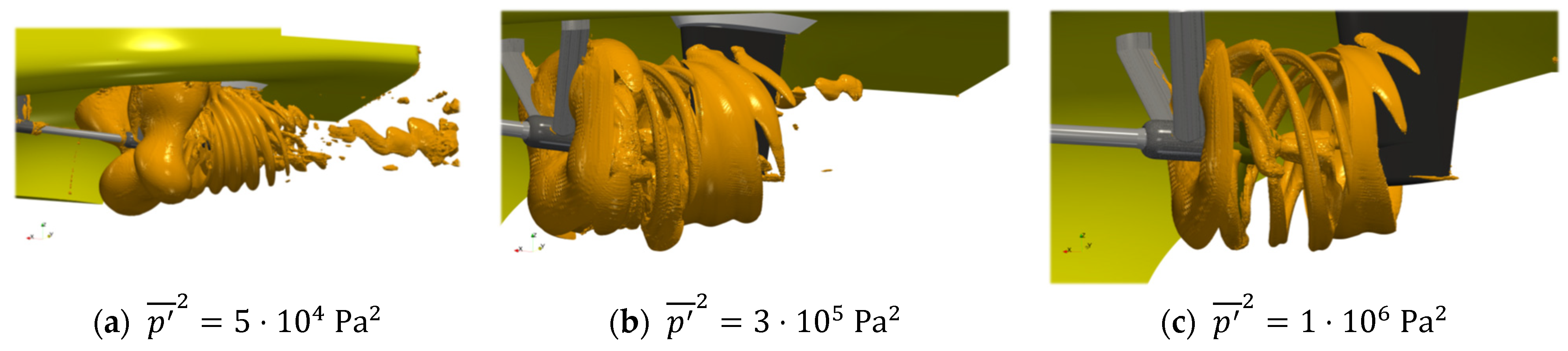
4.3.1. Isosurfaces of Acoustic Sources

In the case of the Proudman acoustic sources, the selection of the isovalues for three-dimensional visualization of relevant acoustic sources is not trivial, therefore several values of the sound power levels $L_w$ are presented and compared in Figure 14. The resulting closed volumes increase when the acoustic power isovalue is set to a lower value. The closed volumes enclose the relevant noise sources related to the selected value. The loudest noise sources in Figure 14a are as expected the propeller blades, the hub vortex, and its interaction with the rudder downstream, in addition to the appendage surfaces of the shaft brackets and the rudder. Unexpectedly, the rudder slipstream towards the ship hull seems to generate noise for a large axial extent downstream of the geometry. This can be attributed to the interaction of the tip vortex with the rudder geometry around the 12 o’clock propeller position, as the comparison with the 6 o’clock position at the same downstream location reveals, where there is no interaction with the rudder geometry, due to the shortened rudder length. Apart from the fact that the rudder is in the slipstream of the propeller, the lower inflow to the propeller and the resulting higher loads at the angular positions of the propeller close to the hull could increase the intensity of the interaction with the rudder.

At lower sound powers in Figure 14b, significantly more details appear as possible acoustic sources. These include a clear overlaying waveform structure on the hub vortex isosurface and a cylindrical shape of noise-generating structure between the shaft brackets and the propeller becomes visible. Also, the tip vortex immediately behind the trailing edge is highlighted, which might only be limited in visualization, by the mesh resolution of the underlying FVM fluid flow simulation. With further higher thresholds for the sound power in Figure 14c,d the tip vortex becomes dominant for all angular positions around the $x$-normal plane through the rudder. The noise generated by the vessel appears only in Figure 14c enclosing a part of the stern section and the transom, meaning that a constant noise level is emitted by the vessel itself, which is plausible as the flow around the hull adjacent regions is not influenced by the propulsor and should be less unsteady.

Another suggestion is to use the pressure second order statistical moments to locate noise sources as illustrated in Figure 15 for several isovalues, which succeeds in highlighting important pressure-based flow features as well as deficiencies in the numerical simulation approach, in particular the sliding mesh approach. It has to be noted that the isosurfaces outside of the sliding mesh are time-invariant once a sufficient number of sample data is exceeded, while inside the rotating mesh region isosurface structures are moving with the propeller such as the tip vortex. The sliding mesh interface is apparent in Figure 15b,c between the propeller and the shaft brackets, and the rudder, respectively. In Figure 15a there are four distinct lobes from the propeller plane upstream on the isosurface, which may indicate a quadrupole noise source of the propulsor or be a result of the interaction with the shaft brackets and the vessels tunnel shape to improve propeller inflow. Especially the tunnel shape is responsible for a large downward extent of the hull boundary layer and thus strong interaction with the propeller as described above.

Behind the propeller, there are several structures indicating the tip vortices and their interaction with the rudder. An identical region as was used for the visualization method of the Proudman acoustic sources downstream of the rudder at the 12 o’clock propeller position is highlighted as a noise source. With the higher isovalue in (b) these details are removed, however, the propeller inside the rotating mesh region can be investigated, and in (c) the hub vortex is also visible.

A classic way to visualize flow features is the vorticity information, such as with the Q-criterion, which is given in Figure 16 around the propeller for a typical isovalue used to highlight the trailing vortices. While it is not strictly connected to acoustic sources, it is indicative of increased turbulence due to the interaction between the main flow field and the hub as well as the tip vortex and possibly relaminarization in the vortex cores. In addition, the interactions between such a complex flow field and the solid surfaces may lead to noise. These interactions may be highlighted such as on the rudder in the image that shows wave-like patterns originating from the location, where the tip vortex of the propeller interacts with the rudder surface. This radial location appears around $0.6-0.7D_P$ from the propeller rotation axis, which corresponds to the region of the maximum thrust of this propeller design. In the image a steady wave of boundary vortices forms, on the rudder surface with a constant wavelength of $~2.5\% D_P$, which would equal an acoustic frequency of $f=290 \mathrm{kHz}$ and is thus outside the frequency range that is typically investigated.

The three options $k$, $Q$, and ${\overline{p^{\prime }}}^2$ for highlighting three-dimensional spatial noise information as isosurfaces are compared side by side in Figure 17 in the fluid volume. Unexpectedly the three options seem to be complementary instead of coinciding, highlighting different regions, and as such are individually not sufficient to indicate all acoustic sources. While the vorticity information favors the trailing vortices, the turbulence information is focused on the leading edge of the blades and the hub vortex, and the second-order statistical moments highlight the upstream directed noise as well as the spurious noise caused by numerical issues at the interface. Again, it is visible that the statistical approach comprises an excellent tool for highlighting discontinuities caused by numerical interpolation, proven by the cloud structures at the downstream interface. Whereas the tip vortex is not captured by $k$, possibly to generally weak vorticity values and possibly relaminarization, the hub vortex features much higher vorticity as it results from the interaction between the five root vortices of the blades. Thus, k by itself is not sufficient to investigate noise sources, with Q seemingly improving the location information. Concluding, these options are valuable as they require minimal post-processing and seem to indicate clearly regions of noise sources, however, they do not allow quantification of any noise emissions.

4.3.2. Lighthill Stresses

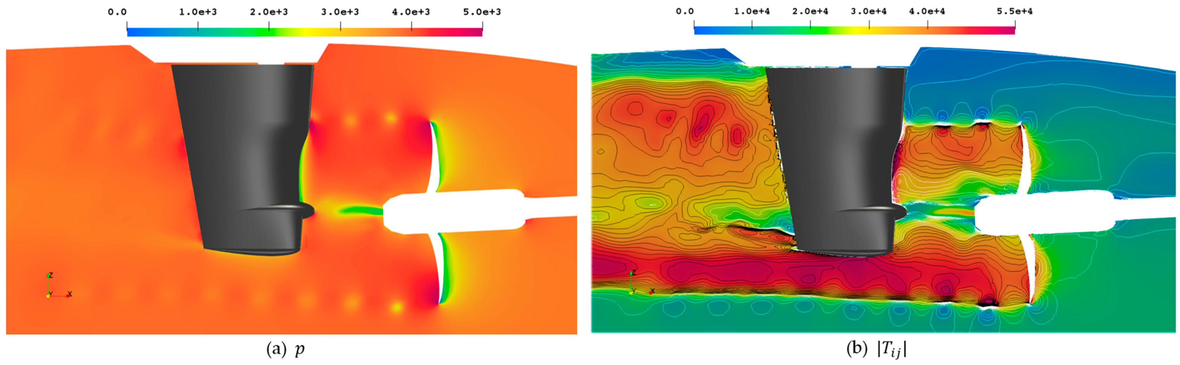
The instantaneous pressure pulse field at a randomly selected timestep is shown in Figure 18 around the propeller hull combination on a midplane through the propeller, with the corresponding instantaneous pressure in Figure 19a around the propeller and the rudder and the Lighthill stress tensor magnitude in Figure 19b. The pressure pulses are a relatively good indicator of noise sources, with the tip vortex and the suction side blades highlighted, as well as the slipstream interaction with the rudder, especially at the lower end, where a trailing vortex from the rudder seems to create rather large acoustic fluctuations, not visible in the isosurface representations in Section 4.3.1. In addition, the downstream interaction with the vessel transom is highlighted here, which is not registered in the other criteria, except Proudman acoustic sources.

While the pressure information in Figure 19a itself is not useful to quantify acoustic emissions, it is indicative of locations of high-pressure gradients, which are attributed to noise emissions. The Lighthill stresses in Figure 19b on the other hand indicate similar regions as the isosurfaces, with strong fluctuations at the tip vortex and the hub vortex, on the propeller blade suction sides, upstream of the rudder around $r/R=0.7$, and behind the rudder at the 12 o’clock position, and in addition below the rudder similar to the pressure pulses in Figure 18. Thus, it seems that this representation combines the highlighted regions from all previous methods and thus proves itself a valuable tool to indicate noise sources.

The Lighthill stress tensor is evaluated from the symmetric fluid compressive stress tensor from Equation (13), shown in Figure 20 for reference, which in turn is obtained from the symmetric perturbation stress tensor from Equation (12) in Figure 21. In the figures, the tensor components are sorted according to their location in a $3\times 3$ matrix, and symmetric tensors are only shown for the upper right side. It has to be noted that the off-diagonal elements experience small value ranges of $\left[-1;1\right]$ compared to the main diagonal with only positive values of $\left[0;5\times {10}^4\right]$, meaning that the colormaps are selected to yield the best visualization and sacrifice comparability between tensor elements.

While the influence of the pressure field is dominating the main diagonal of $P_{ij}$ with almost no difference between the elements, distinct structures appear on the off-diagonal elements, most notably for the rudder interaction as well as quadrupole-like structures in the tip vortex. For the $xy$ element, the slipstream of the rudder is again highlighted at the 12 o’clock position, while $xz$ emphasizes the locations at 6 o’clock and $yz$ shows most notably the features in the hub vortex.

The perturbation stress tensor $P_{ij}^{\prime }$ is deviating from the $P_{ij}$ field on the main diagonal, however, all directional elements $xx$, $yy$, and $zz$ show very similar images compared to each other. The off-diagonal elements again feature a colormap that is different from the main diagonal and the previously used one in Figure 20, to show a different range of details. The value range for the main diagonal is $\left[0;5\times {10}^3\right]$, while the value range for the off-diagonal components is $\left[-0.1;0.1\right]$. In the off-diagonal components, small-scale fluctuations at the sliding mesh interface upstream of the propeller and a slight level jump at the sliding mesh interface at the other ends of the cylinder are visible. It is clearly distinguishable by the eye where the interface is, even without knowing its exact location in advance.

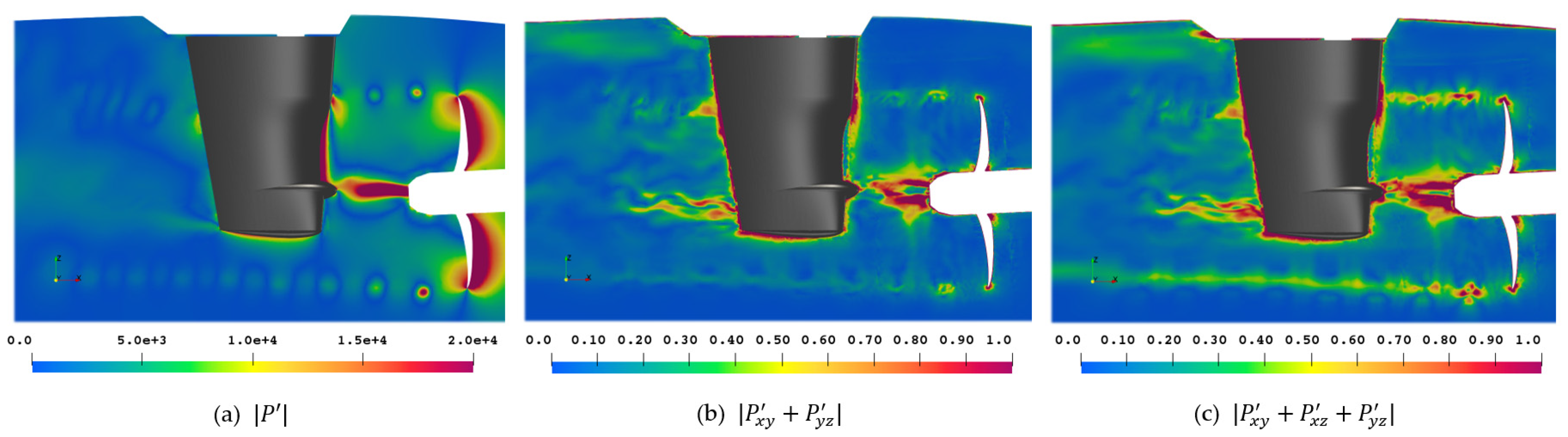
Figure 22 shows the magnitude of all components, which is of course dominated by the main diagonal due to the vastly different value ranges, and the different combinations of off-diagonal components of $P_{ij}^{\prime }$. With this, important noise features become apparent such as the swirls in the tip vortex in (b) and the clover-leaf structure in (c). Also, this is the only way to visualize the numerical issue of the rotating mesh interface, which can be seen in (b) and (c) between the propeller and the rudder. Additionally, the rudder slipstream is accentuated at the expected angular positions.

Finally, the mathematically non-symmetric Lighthill stresses are illustrated in Figure 23, which feature a stronger deviation from the previous stress tensors due to the $\rho u_i{u}_j$ term. Where possible the colormap is kept identical, however, large differences in value range are apparent for the single elements of the tensor. Except for the $xx$ component, all elements feature value ranges with change. Comparing the upper right matrix with the lower left, the symmetry is high, with only the $xz$-$zx$ comparison showing large differences, which have to be addressed by adjusting the colormap. The $xy$-$yx$ element shows the difference between the direction of travel of the blades and therefore the swirl of the slipstream. The off-diagonal components $xz$ and $yz$ and their counterparts in the lower left matrix on the other hand stress exactly the regions, which are also emphasized in the rest of the investigation, meaning there is a clear connection between the noise sources and the visualization by means of Lighthill stresses.

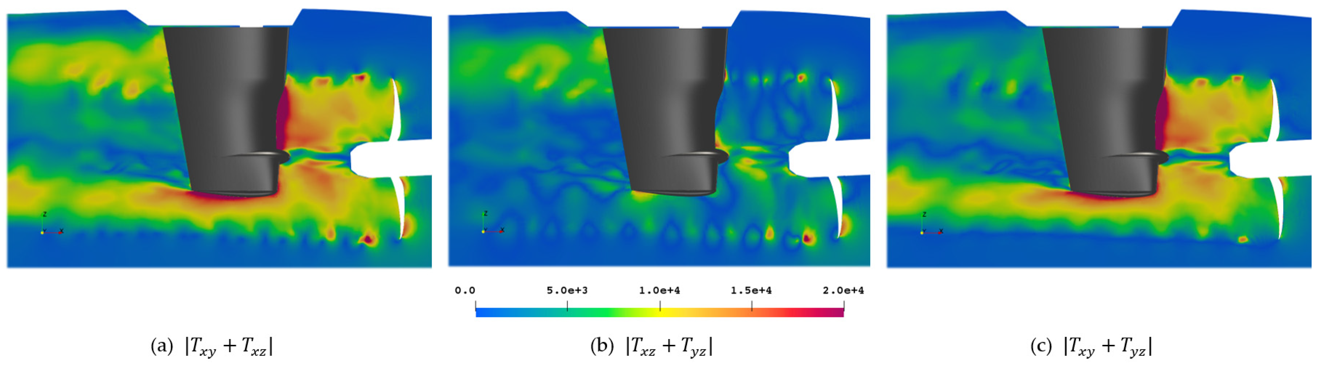
Again, the various combinations of the off-diagonal elements of this matrix are given in Figure 24, which give rise to the expected positions of noise sources. In (a) propeller slipstream and rudder interaction are most prominent. In (b) the propeller tip appears to form a swirl structure upstream, indicating its influence on noise generation. The other highlighted regions are agreeing well with the regions obtained from the Proudman acoustic sources and the statistical moment isosurfaces. This effect can be seen behind the rudder around the 12 o’clock propeller position in Figure 24b, which appears for all three methods. Figure 24c is similar to Figure 24a with a focus on propeller slipstream and rudder interaction.

4.3.3. Directivity

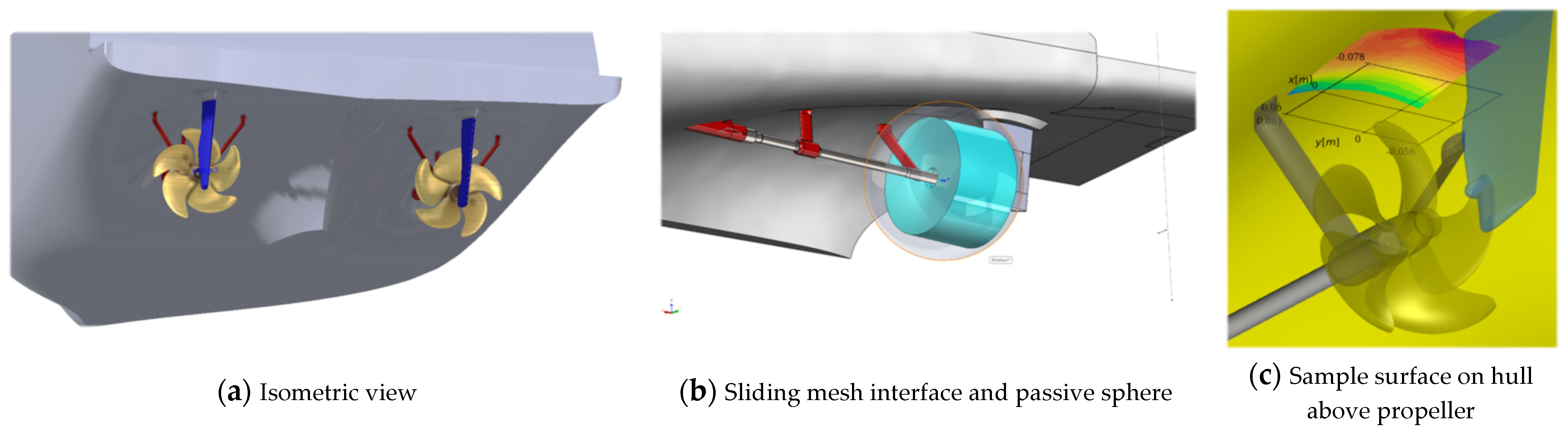
For the investigation of directivity, a passive 3D surface is constructed in the flow field. Since the propeller is the main source of noise, the origin of the coordinate systems used is located at the propeller, as in the simulation, and not at the centerline of the ship. As indicated in Figure 25 a spherical surface is applied with the respective spherical coordinates from $0°–360°$ and the positive axes directed to the bow and outwards. In the simulation, a half-model with a wall at the symmetry plane is considered.

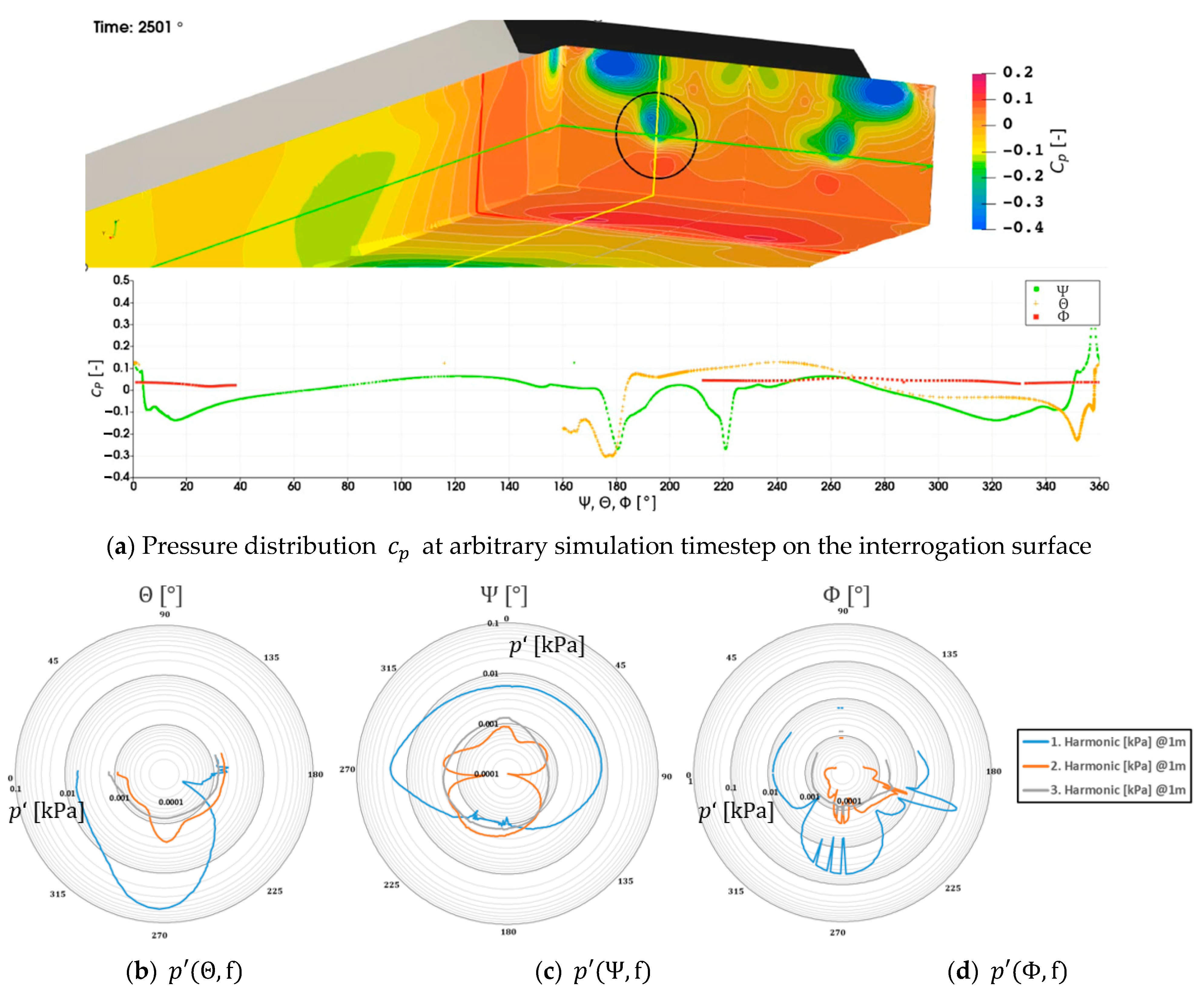
Figure 26a shows the passive spherical surface around the propeller, where the radius of that surface must be large enough to be completely outside the rotating mesh area in order to meet the stationary mesh requirements for post-processing in the frequency. The instantaneous time-variant pressure distribution at an arbitrary converged simulation timestep is visible on the surface and the instantaneous plots along the coordinate dimensions are shown below. The number of waves in the red line along the $\mathsf{\Phi }$ dimension is commensurate with the number of blades and radiates along this dimension dynamically with time. It is noticeable that the pressure distribution does not create symmetrical waves, leading to an increased gradient in front of the leading edge and a decreased gradient behind the passing blade. Both $\mathsf{\Theta }$ and $\mathsf{\Psi }$ dimensions show clear directivity with a low pressure downstream of the propeller hub next to the rudder, with the waterline intersection creating more downstream pressure and the centerline parallel intersection leading to higher pressure towards the vessel. While this instantaneous pressure distribution is useful for understanding the flow field, only a frequency domain investigation obtained from this pressure data over five rotations with a frequency of $f=1°$ and evaluated at the blade passing frequencies provides a time-invariant representation of the emission characteristics. In Figure 26b–d the information about the acoustic propagation along the dimensions is normalized to $r=1 \mathrm{m}$. It has to be noted that the passive surface for the frequency domain analysis is intersected by the rudder and the hull due to technical limitations, which creates gaps in the polar plots that are only partially closed. For the centerline parallel intersection in Figure 26b increased pressure pulses in the direction of the hull are visible for the first three investigated propeller harmonic frequencies, which is thought to be due to the hull reflections, however, with the wavelengths of ${\lambda }_{z=1}\approx 9.2 \mathrm{m}$, ${\lambda }_{z=2}\approx 4.6 \mathrm{m}$ and ${\lambda }_{z=3}\approx 3.1 \mathrm{m}$ neither reflections at the hull nor the domain would be physical. Another possible reason could originate in the wakefield, which creates a deviation in the effective angle of attacks for the propeller in the regions close to the hull, usually lower, possibly leading to different emission characteristics. For the $\mathsf{\Psi }$ direction in Figure 26c, similar trends appear with the pressure pulses increased on the inwards side of the propeller for the first harmonic frequency. In addition, there is a high and strongly fluctuating downstream component in pressure pulses for all displayed frequencies. For Figure 26d the pressure pulses are generally lower and isotropic for the first harmonic, while the higher harmonics show increased downward and downstream directivity. All harmonics have a very strong increase in pressure pulses at the intersection of the interrogation surface with the hull geometry.

A similar analysis is conducted for the rectangular cuboid spanning the complete propeller-hull configuration by mirroring the result at the vessel centerline in Figure 27, which makes the assumption of a monopole point source for adjusting the pressure pulse distance information somewhat questionable. The instantaneous pressure information in Figure 27a with the three intersections along the coordinate dimensions shown in Figure 25 and the propeller diameter projection indicated in black at the aftward side of the cuboid does not show large variations along the surface except for the areas in the propeller wake, visible for the waterline and centerline intersections at $160-220°$. Downstream of the hull above the black circle is a negative pressure area exceeding the values behind the propeller. This does not indicate a larger contribution to emitted noise, as it is only a time snapshot, however, it indicates that the actual wave pattern might deviate strongly from the assumed flat surface, which could have a significant impact on noise propagation.

A more informative insight into the emission characteristics is given by the frequency domain pressure pulses, which due to the distance to the origin have very low values overall, nevertheless, a quantitative comparison is possible. In the polar plots, the left side is the starboard side and care must be taken as the center of the coordinate system is still at the propeller and not midship, which distorts the polar plots slightly in the right half. Starting with Figure 27b along the center line midplane through the origin, the emissions to the bow and downward are larger than to the aft for the first harmonic frequency, which is most likely a result of the scaling to $r=1 \mathrm{m}$ by the assumption of a point source. The higher frequencies show a more uniform directional distribution, with the second harmonic increasing in a downward direction. For the waterline parallel intersection in Figure 27c again the first harmonic is increased in bow direction and shows some fluctuations at the two propeller slipstream intersections at $\mathsf{\Psi }=180°$ and $\mathsf{\Psi }=200°$. For the second harmonic, the emission to the sides of the propeller is very low, creating a distinct directivity towards the aft and the bow, with the first slightly deformed towards the sides. The third harmonic on the other hand has a uniform shape stretching slightly along the direction of travel. In Figure 27d the framewise intersection emission characteristic is given with the first harmonic emitting strongly to the sides and downwards. The peak at $\mathsf{\Phi }=190°$ is most likely a result of the scaling to $r=1 \mathrm{m}$ and the shifted coordinate system through the propeller. The second harmonic shows a similar emission with lower values. The third harmonic on the other hand experiences again an isotropic characteristic. Overall, it is unclear if the absolute values are meaningful with the applied scaling method, however, the emission characteristics give valuable insight into the acoustic interaction between the vessel hull and propulsor.

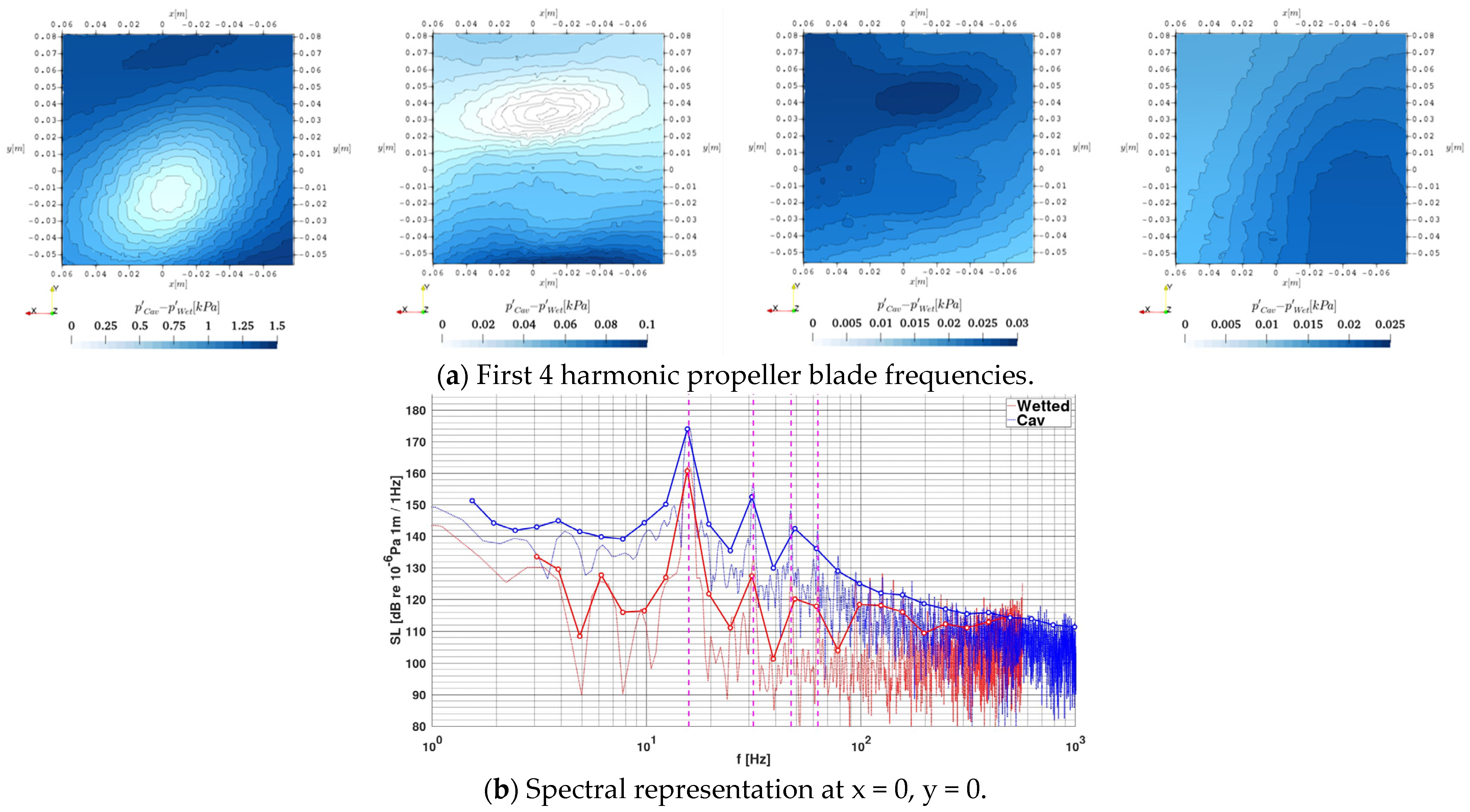
Besides the amplitude information, the phases are of interest in the far-field emissions, if the interaction with other noise sources or reflections from the environment is part of the problem. In Figure 28 the complex phase angle from Equation (17) is plotted as a contour on the sphere presented in Figure 26 and shown isometrically from the upstream direction with the shaftline and from the downstream direction with the vessel and the rudder for the first four propeller blade harmonics $f_z$, respectively. As proposed before the rudder and skeg act as reflection boundaries that detune the phase, when comparing inwards and outwards directed emissions, which is particularly visible for the higher harmonics with a phase difference of around $\pi$ between inwards and outwards directed sound. For the first harmonic the area on the sphere is slightly smaller with only the upwards-directed surfaces on the inwards side showing the phase shift, while otherwise the emission features a uniform phase. The tip vortex radii intersection in the downstream direction at $r/R=1.0$ is distinct for all harmonics, with the higher harmonics increasing the effect radially.

In Figure 29 the complex phase angle with the Fourier-transformed time series obtained by Equation (16) is given on the same rectangular box used in Figure 27 to show the directivity of the phase information to the sea floor, the outside of the vessel and the aft direction, with the transparent propeller-hull combination indicated for orientation. The achieved value range is small with respect to the maximum possible range from $\left[-\pi ;\pi \right]$, indicating a predominantly monopole-like source behavior of the propeller-hull combination. However, there are interesting patterns visible that require detailed analysis. In the view from below the upwards and downward directions of the blades directly below the propeller are visible, see Figure 29c. That is in line with the results presented in Figure 7 on the hull, and in addition a detuning of the phases around $\pi /8$ due to the reflections by the rudder in combination with the skeg of the hull on the inwards side and the half field on the right of the plane $y=0 \mathrm{m}$ are clearly identifiable. A distinct phase shift of $\pi /15$ is visible running across the control surface from the bottom of the rudder to the shaft brackets to the hull along the origin, where the propeller is located, which causes mainly a disparate outward emission to the region in front of the propeller and behind it. In the aft view the detuning by the contained region between the rudder and the skeg of the hull by comparing the half-planes with respect to $y=0 \mathrm{m}$ is again visible. In addition, the turbulent slipstream of the propeller-rudder combination produces a range of phases with a difference of maximum $\pi /5$, which again considering the complete possible value range of the complex phase angle is surprisingly small, however, the chaotic nature of the turbulent mixing is visible in the phases of the sound source representation on the passive surface as well. Comparing this slipstream appearance with the one on the spheres from Figure 28, which intersects mid-rudder and shows a high degree of order, it is clear that the interaction of the propeller slipstream with the rudder creates this chaotic phase emission characteristic downstream.

5. Discussion

With the presented post-processing methods, the sound emission of any noise source may be investigated in more detail than previously possible. Regarding the impact on structures in the vicinity of the acoustic source the classic pressure pulses and corresponding phase information may be obtained in a higher spatial density from CFD simulations in a very common way as this information is part of the solution process of the FVM. With this highly resolved pressure information, more insight into the detailed structures of the acoustic input into the vessel may be obtained than previously possible based on model test results, which rely on a reconstruction from sparse single-point pressure pick-ups. It is shown in this investigation, that this reconstruction might not be as straightforward, as the local pressure distribution is subject to non-linearities above the propeller which are not intuitively recognized. By using statistical methods such as POD, the influence of turbulence and physics may be reduced to achieve a robust information about the acoustic interaction of sources with structures, which may also be extended to arbitrary passive surfaces in the fluid domain such as the one shown in Figure 28 and Figure 29.

For analyzing the volumetric and directional emission characteristics of acoustic sources a more detailed understanding can be achieved with the methods in Section 4.3, which is necessary to have a deep insight into the acoustic propagation. Experiments, especially in full-scale, usually only acquire single-point observer data for investigation of acoustics in the larger fluid domain and thus only generate a very limited insight into the behavior of the acoustic environment of a propeller-hull combination. Further systematic analyses are required to achieve a good understanding of the directionality of these phenomena. With the approach to plot acoustic source information on passive surfaces, the discussion about the spurious noise of FWH permeable surfaces that has long existed in the literature may also be tackled, as the Lighthill stress tensor can be investigated for example in the propeller slipstream to ascertain the optimal length of the closed surface or at sharp edges of the permeable surface to avoid numerical issues. In the context of directional emissions, it is shown that phase information may be important as the complex ship hull shape with its appendages may give rise to a detuning of some frequencies or reflection phenomena between the hull and rudder.

It has to be noted that all presented results have been obtained from only incompressible pressure pulse information of the underlying FVM pressure, which does not take into account any acoustic phenomena. However, it appears that even the incompressible analysis achieves highly valuable information about the possible geometrical structure of the acoustic pressure, which is, in particular, true for the near field and small timesteps of the FVM simulation, where acoustic effects may be neglected as a first approximation.

Once the techniques are sufficiently validated and matured, a consensus may be reached for the visual representation of sound for interpretation in academia and industry, which may lead to standards that can be applied to the design of noise control devices and acoustic suppression mechanisms.

6. Conclusions

In this study a variety of options for visualizing noise for a propeller-hull configuration either as contours on fixed geometrical boundaries or passive surfaces and as three-dimensional isosurfaces are introduced and suggested as an analysis tool. A detailed analysis of the incompressible hull pressure information on a small section of the vessel hull above the propeller is given and analyzed regarding spectral and spatial distribution for a cavitation tunnel and quasi-infinite geometrical simulation setup. The classic representation as pressure pulses gives a good impression of the noise emissions into the vessel hull, which is together with the phase information crucial as an input for structural transmission investigations into the hull. With the POD the general pressure field structure caused by the passing propeller blades can be intuitively visualized and shows a strong invariant to simulation parameters such as turbulence, physics, or domain geometry, supporting the interpretation of simulation results. This may be useful, especially on other vessel surfaces located at critical locations, where the pressure field distribution might be less clear. The energy concentration in the first few POD modes, especially with cavitation might lead to a promising concept of a reduced order model based on machine learning for pressure pulses directly on exchange surfaces, if enough variety of simulation data can be generated, i.e., with different propeller and hull geometries.

Proudman acoustic sources, vorticity information, the second-order statistical moments of the pressure time history, and the turbulent kinetic energy theoretically seem valid options to highlight the three-dimensional local origin of the noise, with the second-order moments being the most useful in the context of CFD simulations, as they equalize short time events and also highlight numerical spurious noise giving the user the possibility to assess the quality of the simulation approach. Here a comparison of different rotating region approaches between arbitrary mesh interface, non-conformal coupling, and overset grid could be very useful in future investigations, if a simulation software suite offers all three options.

The Lighthill stresses are another useful tool to estimate and evaluate sound emissions, as they highlight the combined noise sources detected by the individual other interpretation tools, i.e., the tip vortex and propeller slipstream rudder interaction.

With the help of passive surfaces around objects of interest such as spheres around the propeller, directivity information can be obtained, which can be plotted in two-dimensional polar plots by planar intersections. On active or passive surfaces automated image analysis tools may be used in future investigations to obtain further insight into acoustic source information and be combined with directivity information to receive emission characteristics.

In conclusion, Proudman acoustic sources, statistical moments of pressure, and the Lighthill stress tensor seem to be the most suitable visualization methods for noise to identify acoustic sources for a propeller-hull configuration in three-dimensional space. While Proudman acoustic sources and the Lighthill stress tensor retain the time dimension, the statistical moments on the other hand are useful to highlight numerical issues. Passive surfaces in the simulation are an excellent tool to get directional information on the impact of sound sources.

References

1. Frisk, G.V. Noiseonomics: The Relationship between ambient noise levels in the sea and global economic trends. Sci. Rep. 2012, 2, 437. [Google Scholar] [CrossRef] [PubMed] [Green Version]
2. Erbe, C. Underwater Acoustics: Noise and the Effects on Marine Mammals. In Effects of Anthropogenic Noise on Animals; JASCO Applied Sciences: Silver Spring, MD, USA, 2018; pp. 227–309. [Google Scholar]
3. Lidtke, A.; Klapwijk, M.; Lloyd, T. Scale-Resolving Simulations of a Circular Cylinder Subjected to Low Mach Number Turbulent Inflow. J. Mar. Sci. Eng. 2021, 9, 1274. [Google Scholar] [CrossRef]
4. Francescantonio, P.D. A New Boundary Integral Formulation for The Prediction of Sound Radiation. J. Sound Vib. 1997, 202, 491–509. [Google Scholar] [CrossRef]
5. Liefvendahl, M.; Bensow, R. Simulation-Based Analysis of Flow-Generated Noise from Cylinders with Different Cross-Sections. In Proceedings of the 32nd Symposium on Naval Hydrodynamics, Hamburg, Germany, 5–10 August 2018. [Google Scholar]
6. Sezen, S.; Atlar, M.; Fitzsimmons, P. Prediction of cavitating propeller underwater radiated noise using RANS & DES-based hybrid method. Ships Offshore Struct. 2021, 4, 93–105. [Google Scholar]
7. Yilmaz, N.; Atlar, M.; Fitzsimmons, P. An Improved Tip Vortex Cavitation Model for Propeller-Rudder Interaction. In Proceedings of the 10th International Cavitation Symposium, Baltimore, MD, USA, 14–16 May 2018. [Google Scholar]
8. Posa, A.; Broglia, R.; Felli, M. Acoustic signature of a propeller operating upstream of a hydrofoil. Phys. Fluids 2022, 34, 065132. [Google Scholar] [CrossRef]
9. Yilmaz, N.; Aktas, B.; Sezen, S.; Atlar, M.; Fitzsimmons, P.; Felli, M. Numerical Investigations of Propeller-Rudder-Hull Interaction in the Presence of Tip Vortex Cavitation. In Proceedings of the smp’19, Rome, Italy, 26–30 May 2019. [Google Scholar]
10. Kimmerl, J.; Abdel-Maksoud, M.; Nataletti, M.; Savio, L. Acoustic Comparison of a Ship-Propeller Model in Cavitating Conditions with LES and FWH-Method. In Proceedings of the Seventh International Symposium on Marine Propulsors, Wuxi, China, 17–21 October 2022. [Google Scholar]
11. Brouwer, J.; Tukker, J.; Klinkenberg, Y.; van Rijsbergen, M. Random uncertainty of statistical moments in testing: Mean. Ocean. Eng. 2019, 182, 563–576. [Google Scholar] [CrossRef]
12. Lidtke, A.; Lloyd, T.; Lafeber, F.; Bosschers, J. Predicting cavitating propeller noise in off-design conditions using scale-resolving CFD simulations. Ocean. Eng. 2022, 254, 111176. [Google Scholar] [CrossRef]
13. Liu, Y.; Li, Y.; Shang, D. The Generation Mechanism of the Flow-Induced Noise from a Sail Hull on the Scaled Submarine Model. Appl. Sci. 2018, 9, 106. [Google Scholar] [CrossRef] [Green Version]
14. Göttsche, U.; Lampe, T.; Scharf, M.; Abdel-Maksoud, M. Evaluation of Underwater Sound Propagation of a Catamaran with Cavitating Propellers. In Proceedings of the Sixth International Symposium on Marine Propulsors, Rome, Italy, 26–30 May 2019. [Google Scholar]
15. Kimmerl, J.; Mertes, P.; Krasilnikov, V.; Koushan, K.; Savio, L.; Felli, M.; Abdel-Maksoud, M.; Göttsche, U.; Reichstein, N. Analysis Methods and Design Measures for the Reduction of Noise and Vibration Induced by Marine Propellers. In Proceedings of the 23rd International Congress on Acoustics, Aachen, Germany, 9–13 September 2019. [Google Scholar]
16. Schnerr, G.; Sauer, J. Physical and Numerical Modeling of Unsteady Cavitation Dynamics. In Proceedings of the ICMF-2001, 4th International Conference on Multiphase Flow, New Orleans, LA, USA, 27 May–1 June 2001. [Google Scholar]
17. Gerasimov, A. Quick Guide to Setting Up LES-Type Simulations. Available online: ANSYS Customer Portal.
18. Bogey, C.; Bailly, C.; Juvé, D. Noise investigation of a high subsonic, moderate Reynolds number jet using a compressible large eddy simulation. Theor. Comput. Fluid Dyn. 2003, 16, 273–297. [Google Scholar] [CrossRef]
19. Tanigawa, R.; Yatabe, K.; Oikawa, Y. Experimental visualization of aerodynamic sound sources using parallel phase-shifting interferometry. Exp. Fluids 2020, 61. [Google Scholar] [CrossRef]
20. Bogey, C.; Bailly, C.; Juvé, D. Noise computation using Lighthill’s equation with inclusion of mean flow-acoustics interactions. In Proceedings of the 7th AIAA/CEAS Aeroacoustics Conference and Exhibit, Maastrich, The Netherlands, 28–30 May 2001. [Google Scholar]
21. ESI Group. OpenFOAM User Guide; OpenCFD Ltd.: Berkshire, UK, 2023; Available online: www.openfoam.com (accessed on 15 February 2023).
22. Ringwall. Aeroacoustic Sound Sources Around the Wheels of a Passenger Car. Master’s Thesis, Department of Applied Mechanics, Chalmers University of Technology, Gothenburg, Sweden, 2017. [Google Scholar]
23. Weiss, J. A Tutorial on the Proper Orthogonal Decomposition. In AIAA Aviation Forum; AIAA ARC: Dallas, TX, USA, 2019. [Google Scholar]
24. Zigunov, F. POD—Proper Orthogonal Decomposition (Wrapper); MATLAB Central File Exchange: Natick, MA, USA, 2019. [Google Scholar]
25. Kimmerl, J.; Mertes, P.; Krasilnikov, V.; Koushan, K.; Savio, L.; Felli, M.; Abdel-Maksoud, M.; Reichstein, N. Experimental and Numerical Advances in Underwater Radiated Noise Prediction of Cavitating Propeller-Hull Combinations. In Proceedings of the 24th International Congress on Acoustics, Gyeongju, Republic of Korea, 24–28 October 2022. [Google Scholar]
Figure 1. Test case 3D-model.
Jmse 11 00834 g001
Figure 2. Midplane of cavitation tunnel and quasi-infinite domain.
Jmse 11 00834 g002
Figure 3. First 4 harmonic propeller blade frequencies incompressible hull pressure above propeller, comparison of domain extent, RANS without cavitation.
Jmse 11 00834 g003
Figure 4. First 4 harmonic propeller blade frequencies incompressible hull pressure above propeller, comparison of domain extent, RANS with cavitation.
Jmse 11 00834 g004
Figure 5. First 4 harmonic propeller blade frequencies incompressible hull pressure above propeller, comparison of domain extent, LES with cavitation.
Jmse 11 00834 g005
Figure 6. Difference between cavitating and non-cavitating simulation.
Jmse 11 00834 g006
Figure 7. Phase information on hull at the first 4 harmonic propeller blade harmonic frequencies, comparison of domain extent, and RANS.
Jmse 11 00834 g007
Figure 8. Phase information on hull at the first 4 harmonic propeller blade harmonic frequencies, comparison of domain extent, RANS with cavitation.
Jmse 11 00834 g008
Figure 9. Phase information on hull at the first 4 harmonic propeller blade harmonic frequencies, comparison of domain extent, LES with cavitation.
Jmse 11 00834 g009
Figure 10. First 4 POD modes of pressure time data set on hull above propeller, comparison of domain extent, RANS.
Jmse 11 00834 g010
Figure 11. First 4 POD modes of pressure time data set on hull above propeller, comparison of domain extent, RANS with cavitation.
Jmse 11 00834 g011
Figure 12. First 4 POD modes of pressure time data set on hull above propeller, comparison of domain extent, LES with cavitation.
Jmse 11 00834 g012
Figure 13. POD mode energies of the first 5 modes.
Jmse 11 00834 g013
Figure 14. Comparison of Proudman acoustic power 3D isovalue around propulsor and rudder.
Jmse 11 00834 g014
Figure 15. Second order statistical moments of pressure time history.
Jmse 11 00834 g015
Figure 16. Near Wall Q-criterion Q = 5 10 4   s 2 isosurface on shaft brackets, propeller, and rudder.
Jmse 11 00834 g016
Figure 17. Comparison of isosurfaces of turbulent kinetic energy k = 1.5   m 2 / s 2 (purple), second order statistical moments of pressure time history p ¯ 2 = 1 10 6   Pa 2   (orange), and Q-criterion Q = 5 10 4   s 2 (green) around rotating mesh region and sliding mesh interface.
Jmse 11 00834 g017
Figure 18. Instantaneous pressure pulses p in [ Pa ] at arbitrary converged timestep on the midplane.
Jmse 11 00834 g018
Figure 19. Instantaneous pressure p in [ Pa ] at arbitrary converged timestep on midplane through the propeller and corresponding Lighthill stress tensor magnitude | T i j | in [ Kg / ms 2 ].
Jmse 11 00834 g019
Figure 20. Fluid compressive stress tensor P i j in [ Kg / ms 2 ].
Jmse 11 00834 g020
Figure 21. Perturbation stress tensor P i j in [ Kg / ms 2 ].
Jmse 11 00834 g021
Figure 22. Perturbation stress tensor P i j magnitude (a) and magnitude of off-diagonal components (b,c) on midplane in [ Kg / ms 2 ].
Jmse 11 00834 g022
Figure 23. Lighthill stress tensor T i j in [ Kg / ms 2 ].
Jmse 11 00834 g023
Figure 24. Lighthill stress tensor T i j magnitude of off-diagonal components in [ Kg / ms 2 ].
Jmse 11 00834 g024
Figure 25. Definition of the spherical coordinate system for the directivity investigation.
Jmse 11 00834 g025
Figure 26. Directivity of harmonic frequencies on a passive sphere around the propeller.
Jmse 11 00834 g026
Figure 27. Directivity of harmonic frequencies on the passive rectangular box around propeller-hull combination.
Jmse 11 00834 g027
Figure 28. Complex phase angle information on the passive sphere from Figure 26.
Jmse 11 00834 g028
Figure 29. Complex phase angle information at f Z = 1 on the passive rectangular box shown in Figure 27.
Jmse 11 00834 g029