Ocean Surface Gravity Wave Evolution during Three Along-Shelf Propagating Tropical Cyclones: Model’s Performance of Wind-Sea and Swell

Abstract

Despite recent advancements in ocean–wave observations, how a tropical cyclone’s (TC’s) track, intensity, and translation speed affect the directional wave spectra evolution is poorly understood. Given the scarcity of available wave spectral observations during TCs, there are few studies about the performance of spectral wave models, such as Simulating Waves Nearshore (SWAN), under various TC scenarios. We combined the National Data Buoy Center observations and numerical model hindcasts to determine the linkages between wave spectrum evolution and TC characteristics during hurricanes Matthew 2016, Dorian 2019, and Isaias 2020. Five phases were identified in the wave spectrogram based on the normalized distance to the TC, the sea–swell separation frequency, and the peak wave frequency, indicating how the wave evolution relates to TC characteristics. The wave spectral structure and SWAN model’s performance for wave energy distribution within different phases were identified. The TC intensity and its normalized distance to a buoy were the dominant factors in the energy levels and peak wave frequencies. The TC heading direction and translation speed were more likely to impact the durations of the phases. TC translation speeds also influenced the model’s performance on swell energy. The knowledge gained in this work paves the way for improving model’s performance during severe weather events.

1. Introduction

Tropical cyclones (TCs) affecting the U.S. East Coast are ubiquitous in the hurricane seasons. As storms approach coastal areas, gravity waves and increased total water levels (TWL = mean sea level plus astronomic tides plus storm surge plus wave runup) can cause significant damage because of erosion, barrier–island breaching, and coastal flooding [1,2]. The National Oceanic and Atmospheric Administration (NOAA) [3] indicated that as coastal counties along the U.S. East Coast have experienced remarkable increases in population and economic activities, potential damage caused by TCs may rise dramatically. The 2021 report of the Intergovernmental Panel on Climate Change (IPCC) [4] concluded that strong TCs were expected to be more probable in the future and that their translation speeds were likely to vary.

Gravity waves are key to sediment transport, impact dunes and infrastructure (e.g., buildings and roads), and affect TWLs through wave setup, infragravity wave generation, and swash motions. Gravity wave generation and propagation processes during TCs are complex. Depending on the location relative to the eye of the TCs, the wave field is composed of different wave components (sea and swell), with varying relative intensities and directions. The sea primarily consists of high-frequency waves generated by local wind, while the swell mainly contributes to wave energy at low frequencies [5]. Under extreme weather events, the statistical wave bulk parameters (e.g., zero-moment wave height, mean wave direction, and peak wave period) are not sufficient to describe the sea state composed of complex wave systems in the open ocean, in which wave–wave interactions dominate [6]. To isolate the sea and swell from the wave frequency spectrum, many different strategies have been suggested. While in some methods, the separation of sea and swell depends on wave characteristics [7,8], others depend on the wind intensity [9]. There are also algorithms that consider the effect of both wind intensity and wave characteristics [5,10]. Whereas some previous efforts [8,11] have compared the performance of different sea–swell separation methods, the performance and sensitivity of these approaches to separate the sea and swell components under different extreme weather conditions are poorly understood.

Improvements to a nearshore hydrodynamic simulation intrinsically require a better understanding of the performance of wave generation and propagation models in capturing the temporal and spatial evolution of the directional wave spectrum. Ref. [12] explained how the misalignment between wind and wave directions was affected by TC translation speeds during Hurricane Bonnie (1998). However, ref. [12] did not discuss the effects of TC intensity and size on such misalignment. Ref. [13] compared the instantaneous wind and wave vector fields in different quadrants of hurricanes referenced to the center of the hurricane, the heading direction, and the radius of maximum wind. Ref. [13] reported that the mean directions of wind and waves might experience significant differences in the rear-left (RL) quadrant, and the directional wave spectrum usually became multi-modal. Ref. [14] presented the spectral analysis during historical typhoons in the West Pacific Ocean. They analyzed the timing and conditions when the spectrum became bi-modal. Ref. [6] used the Simulating Waves Nearshore model (SWAN) [15] to study the evolution of the wave spectrum components and found that the wave field under TCs depended on the forward motion (TC heading direction and TC translation speed) instead of following the instantaneous wind speed and the radius of maximum wind alone. While the aforementioned studies focused on historical storms affecting different geographical locations and used different models and/or observations, a comprehensive comparison of the wave spectral characteristics at the same geographic location during various storm events and an analysis of the performance of a specific model are necessary.

Coupled ocean–wave numerical models solving for physics including wind, atmospheric pressure, TWLs, current velocities, wave fields, and their interactions facilitated the analysis of the potential hazards associated with TCs. SWAN was developed and widely used to resolve the temporal and spatial evolution of directional wave spectra. Relevant works, such as ref. [16], documented some limitations and possible drawbacks of SWAN to resolve specific wave physics. Ocean circulation models, such as the Regional Ocean Modeling System (ROMS) [17], simulate 3-dimensional ocean circulation, astronomic tides, and storm surges. Refs. [18,19] developed the Coupled Ocean–Atmosphere–Wave–Sediment Transport modeling system (COAWST), coupling a 3-dimensional oceanic model (ROMS), an atmospheric model (Weather Research and Forecasting model, WRF), two wave models (SWAN and WAVEWATCH III), and a sediment transport model named Community Sediment Transport Modeling System (CSTMS). While the radiation stresses approach was widely used for wave-induced currents, especially in the surf zone [20,21], ref. [22] included the vortex-force formalism for the wave–current interaction in the COAWST modeling system. The vortex-force formalism was tested to well reproduce wave–current interaction in a tidal inlet [23]. Ref. [24] applied COAWST to analyze the effects of wave–current interaction between wind waves and the Gulf Stream around the South Atlantic Bight (SAB) during Hurricane Matthew (2016). The Gulf Stream was found to increase wave energy dissipation and reduce wave energy by decreasing the potential for an extended wave generation fetch. Ref. [24] also verified that the statistical wave bulk parameters during Matthew were well reproduced by COAWST.

TCs traveling along the coastline can lead to significantly different surge and swell propagation processes than landfalling TCs [25]. Additionally, the typical features of storm tracks across different ocean basins and latitudes may differ [26]. The spatial and temporal evolution of the directional wave spectra during various TCs is poorly understood, especially in those TCs traveling along the coast. In this study, we analyzed the evolution of the directional wave spectra and determined the SWAN model’s performance for wave spectrum during recent along-shelf propagating TCs (Matthew 2016, Dorian 2019, and Isaias 2020) within the SAB.

The comparison of the wave fields during these three TCs provided the opportunity to analyze the linkages between TC characteristics and wave spectral evolution. We investigated the relationship between the TC translation speed, intensity, normalized distance to the eye, and the spatial structure of directional wave spectra. The advanced techniques developed in previous works [6,13,14,27] provided examples and approaches for a wave spectral analysis and were synthesized and applied in the present work. Despite the similar tracks, the atmospheric characteristics of hurricanes Matthew, Dorian, and Isaias were different around the SAB, which made the distributions of TWLs along the SAB during these TCs significantly different [2].

This paper is organized as follows: a review of three historical TCs (Matthew 2016, Dorian 2019, and Isaias 2020) is presented following the introduction. In the next section, we briefly introduce the modeling system and setup applied in this work. Model verification based on the comparison with historical observations can be found next. Finally, a spectrum analysis and a discussion of air–sea interactions are presented.

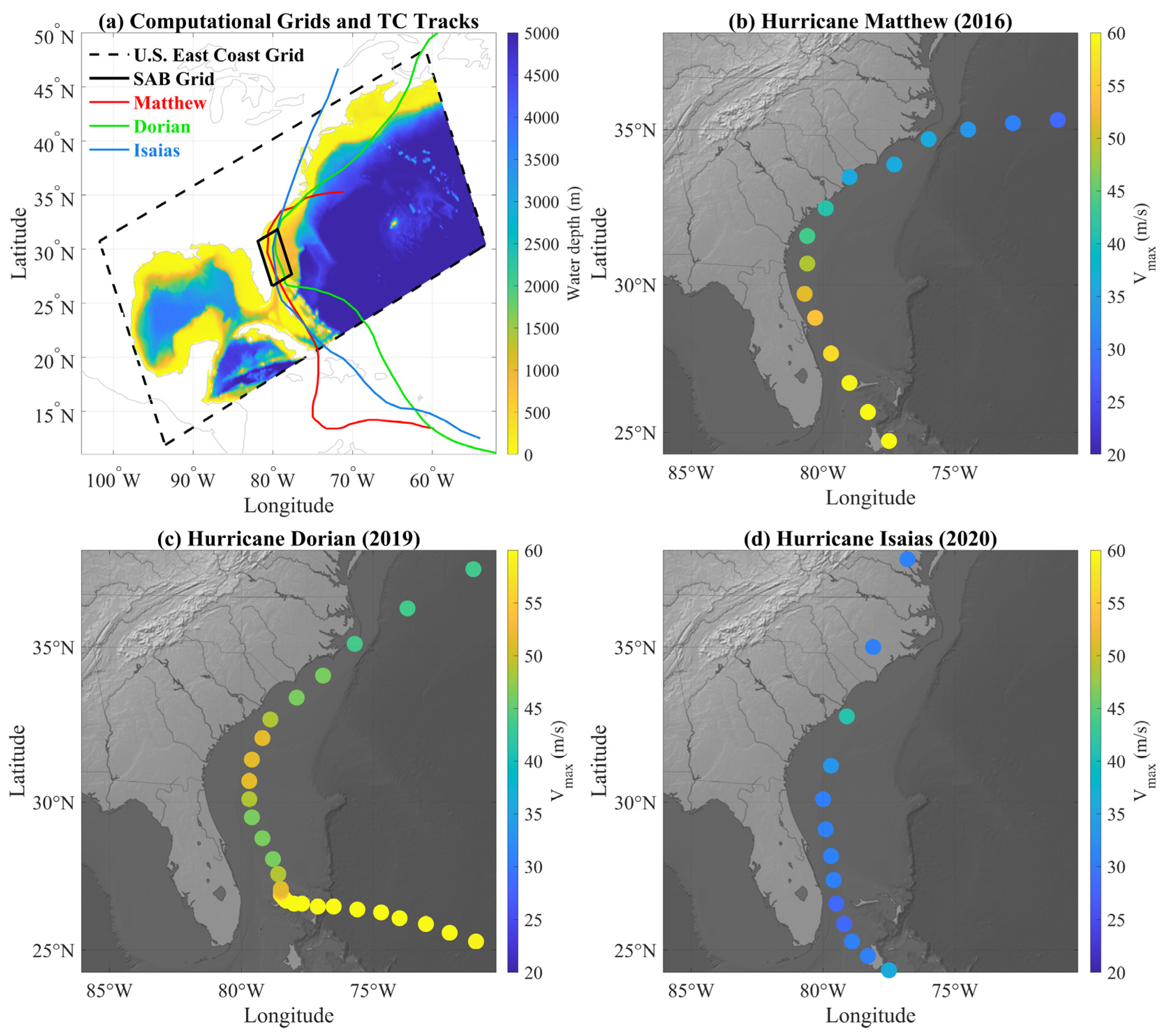
2. Study Area and the TCs of Interest

Extending from the upper Florida Keys to Cape Hatteras in North Carolina, the width of the SAB continental shelf ranges from 40 km to 140 km, with the Gulf Stream flowing at 2.0 $\mathrm{m}{\mathrm{s}}^{-1}$ to 2.5 $\mathrm{m}{\mathrm{s}}^{-1}$ along the shelf break. Hurricanes Matthew, Dorian, and Isaias had similar tracks when propagating over the SAB, as shown in Figure 1b–d. We employed the re-analyzed TC track data from the International Best Track Archive for Climate Stewardship (IBTrACS; https://ibtracs.unca.edu/index.php?name=introduction; accessed on 31 March 2023). The IBTrACS dataset offers information on the best-track tropical cyclones worldwide, gathered from organizations in all ocean basins. The World Meteorological Organization has approved the initiative as the official archive and distribution channel for best-track TC data. Based on the Saffir–Simpson Hurricane Wind Scale (SSHWS), Matthew and Dorian were major Atlantic hurricanes impacting the SAB (i.e., category 4), whereas Isaias reached category 1 at its peak. Isaias had a faster translation speed than the other two hurricanes within the SAB, while Dorian’s translation speed was the slowest (

Table 1. Mean values of TC parameters of the three historical hurricanes within the SAB (values calculated from IBTrACS data). $V_t$ is the translation speed of storms; $V_{max}$ is the maximum sustained wind; $P_{min}$ is the minimum atmospheric pressure; and $R_{max}$ is the radius of maximum wind.

Hurricane	${\mathit{V}}_{\mathit{t}}\left(\mathbf{m}{\mathbf{s}}^{-1}\right)$	${\mathit{V}}_{\mathit{m}\mathit{a}\mathit{x}}\left(\mathbf{m}{\mathbf{s}}^{-1}\right)$	${\mathit{P}}_{\mathit{m}\mathit{i}\mathit{n}}\left(\mathbf{m}\mathbf{b}\right)$	${\mathit{R}}_{\mathit{m}\mathit{a}\mathit{x}}\left(\mathbf{k}\mathbf{m}\right)$
Matthew	6.17	45.25	959.44	52.67
Dorian	3.27	58.80	945.36	35.52
Isaias	6.26	32.11	993.06	53.38

). The present work focused on these three TCs because of their similar tracks propagating along the continental shelf within the SAB but with different $V_t$ (TC translation speeds), $R_{max}$ (radii of maximum wind), and $V_{max}$ (TC maximum sustained wind speeds).

Hurricane Matthew reached hurricane status by 18:00 UTC 29 September 2016, according to National Hurricane Center’s report [28]. Around 00:00 UTC 07 October 2016, Matthew made landfall in Grand Bahama Island as an SSHWS category 4 hurricane. The observed $V_{max}$ was 60 $\mathrm{m}{\mathrm{s}}^{-1}$ during its landfall in the Bahamas, whereas the central pressure was as low as 937 mb. At the time that Matthew entered the SAB, its $V_t$ was 6.21 $\mathrm{m}{\mathrm{s}}^{-1}$ (heading toward 32.19$°$, counter-clockwise to north) at 01:00 UTC 07 October 2016. After entering the SAB, the observed $V_{max}$ decreased to 54 $\mathrm{m}{\mathrm{s}}^{-1}$. Traveling along the U.S. East Coast, Matthew made another landfall in South Carolina and propagated offshore again. Moving east–northeast, Matthew weakened to a tropical storm during 10 October 2016.

In 2019, Dorian became a hurricane around the eastern tip of St. Croix in the U.S. Virgin Islands at 15:30 UTC 28 August 2019 [29]. It continued to travel toward the northwest and made landfall in the Bahamas as an SSHWS category 5 hurricane around 16:40 UTC 1 September 2019. The observed $V_{max}$ at landfall was 82 $\mathrm{m}{\mathrm{s}}^{-1}$, with its central pressure of 910 mb. The eye moved with a $V_t$ of 0.62 $\mathrm{m}{\mathrm{s}}^{-1}$ (heading toward the true north) at 06:00 UTC on 3 September 2019 while entering the SAB. The translation speed of Dorian was slowest when passing over the SAB. During its passage through the SAB, Dorian traveled along a path that was like Matthew’s best-track, but more displaced to the offshore (96.21 km on average). Its intensity decreased due to the landfall in the Bahamas, but strengthened again as it entered the SAB. Meanwhile, the observed $V_{max}$ was 47 $\mathrm{m}{\mathrm{s}}^{-1}$.

Isaias became a tropical cyclone on 30 July 2020, south of the Dominican Republic, and further strengthened into a tropical storm [30]. Around 00:00 UTC 1 August 2020, Isaias became an SSHWS category 1 hurricane. Its central atmospheric pressure was 987 mb with $V_{max}=3$9 $\mathrm{m}{\mathrm{s}}^{-1}$ at that instant. Like Dorian, Isaias weakened when passing through the Bahamas, but strengthened again as it traveled northward. The observed $V_{max}$ was 31 $\mathrm{m}{\mathrm{s}}^{-1}$. Isaias reached $V_t$ of 7.00 $\mathrm{m}{\mathrm{s}}^{-1}$ heading toward the SAB, when it was located around the Island of Hispaniola. Then, the $V_t$ of Isaias reached its minimum (3.11 $\mathrm{m}{\mathrm{s}}^{-1}$) at 02:00 UTC 2 August 2020 and kept accelerating afterward. Overall, Isaias had the weakest $V_{max}$ and the fastest $V_t$ during its passage over the SAB among the three historical TCs.

3. Numerical Model Description and Setup

Following the modeling framework of ref. [24], we configured COAWST as a coupled ocean–wave model. The ocean dynamics are resolved with ROMS, while wind wave generation and propagation are simulated with SWAN. The ocean and wave models use the same horizontal grids, with a 5 km resolution parent grid covering the entire U.S. East Coast and a 1 km resolution child grid covering the southern SAB.

3.1. Ocean Model (ROMS)

The Regional Ocean Modeling System (ROMS) is the ocean circulation model in COAWST. The finite-difference approximations of the Reynolds Averaged Navier–Stokes equations (RANS) are solved on the numerical scheme of ROMS using a 3-dimensional terrain-following framework with a curvilinear coordinate transformation [17]. Further details of the forcing in the governing equations of ROMS can be found in refs. [18,19,22].

3.2. Wave Model (SWAN)

SWAN [15] is a third-generation spectral wave model that solves the wave action evolution by considering the refraction, shoaling, wave–current interactions, wind wave generation, and various wave energy dissipation (bottom friction, breaking, and white-capping). The semi-empirical formula developed from the JONSWAP (Joint North Sea Wave Project) results is activated for bottom friction dissipation [31]. We use the formulas proposed by ref. [32] to consider wind wave growth and white-capping. For the non-linear quadruplet wave–wave interaction, we employ the discrete interaction approximation (DIA) of ref. [33].

3.3. Model Coupling Scheme

In COAWST, water levels, current velocities, and wave fields are two-way coupled using the Model Coupling Toolkit [34]. A 30-min coupling interval is used to exchange data between ROMS and SWAN including the water surface elevation, current velocities, zero-moment wave heights, peak wavelength, peak wave period, and mean wave direction. This data exchange interval follows the settings of ref. [24], which is sufficient for simulating the offshore wave spectrum. Details for the coupling technique and exemplary case study can be found in refs. [18,19]. At the sea surface, the sea surface roughness [35] and the wind shear stresses are calculated and used to force the ocean model. The vortex-force method [22] is employed to consider the wave–current interaction. The use of vortex-force formalism is significant, especially under scenarios where the vertical structure of wave-driven flows is important. The wave and current boundary layer characteristics are calculated using the SSW_BBL option, which applies the model proposed by ref. [36].

3.4. Model Setup

ROMS is forced with winds and atmospheric pressure derived from the Rapid refresh (RAP) reanalysis (https://www.nco.ncep.noaa.gov/pmb/products/rap/; accessed on 18 August 2020). This dataset includes wind velocities that are 10 m above the mean sea level (MSL) and atmospheric pressure at MSL. RAP has a spatial resolution of 13 km with a 1-h time interval, but it does not cover the entire computational domain. Offshore areas that are not covered by RAP are filled with wind and atmospheric pressure forces from the Global Forecast System (GFS) (50 km resolution with a 3-h time interval; https://www.ncdc.noaa.gov/data–access/model–data/model–datasets/global–forcast–system–gfs; accessed on 18 August 2020).

The U.S. East Coast domain has a horizontal grid resolution of 5 km with 896 ($\xi$– direction) $\times$336 ($\eta$–direction) grid cells. The SAB domain has a horizontal grid resolution of 1 km with 272 ($\xi$−direction) $\times$ 376 ($\eta$−direction) grid cells. ROMS numerical grids have 16 vertical layers. The baroclinic time steps in ROMS are 30 s and 15 s for the U.S. East Coast grid and the SAB grid, respectively. We apply the re-analyzed data from Hybrid Coordinate Ocean Model (HYCOM; https://www.hycom.org/dataserver/gofs-3pt1/analysis; accessed on 31 March 2023) to obtain initial conditions for the water levels, velocities, salinity, and temperature. As for the astronomic tides, 13 tidal constituents (M2, S2, N2, K1, K2, O1, P1, Q1, MF, MM, M4, MS4, and MN4) from Oregon State University TPXO Tide Model database (https://www.tpxo.net/home; accessed on 31 March 2023) are applied to the parent grid. To radiate out deviations from exterior values at the speed of the external gravity waves, the Flather boundary condition is used at the offshore boundaries of the ROMS model (the northeast and southeast boundaries of the black dashed line box in Figure 1a) for the momentum balance. We run simulations for 11 days with a 2-day spin-up (i.e., 13 days in total). The 2-day spin-up has been tested to be sufficient for the initial conditions (e.g., currents, water levels, temperature, and salinity) to reach the equilibrium state in our model. An 11-day simulation period (including at least 5 days before the peak of the storm) is tested to be long enough to observe the generation and propagation of swells toward the SAB at all buoys.

For the boundary conditions of SWAN model, statistical wave bulk parameters (zero-moment wave height, mean wave direction, and peak wave period) from NOAA’s WAVEWATCH III re-analyzed global dataset (https://polar.ncep.noaa.gov/waves/ensemble/download.shtml; accessed on 31 March 2023) are imposed at 47 boundary segments along the southeast and northeast boundaries of the U.S. East Coast grid (the black dashed line box in Figure 1a) hourly, assuming the JONSWAP (Joint North Sea Wave Project) wave spectra as the boundary conditions for the model setup in the case of Hurricane Matthew. NOAA’s WAVEWATCH III re-analyzed global dataset does not have available data during Dorian and Isaias. Thus, we employ a larger grid to cover the North Atlantic Ocean and the Gulf of Mexico with our modeling system to generate the wave boundary conditions for these two TCs. The wave spectrum is solved with 60 and 25 directional and frequency bins, respectively. The parent and child grids are solved with 30 and 15 s as their computational time steps, respectively. As for the atmospheric forcing, SWAN uses the same GFS–RAP input as ROMS.

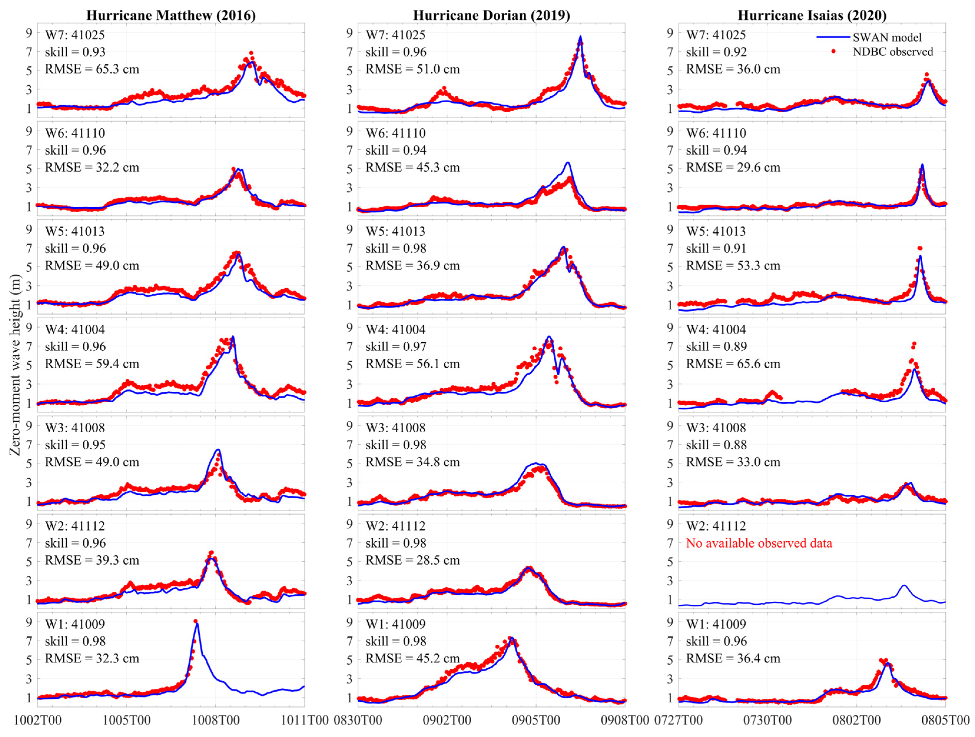
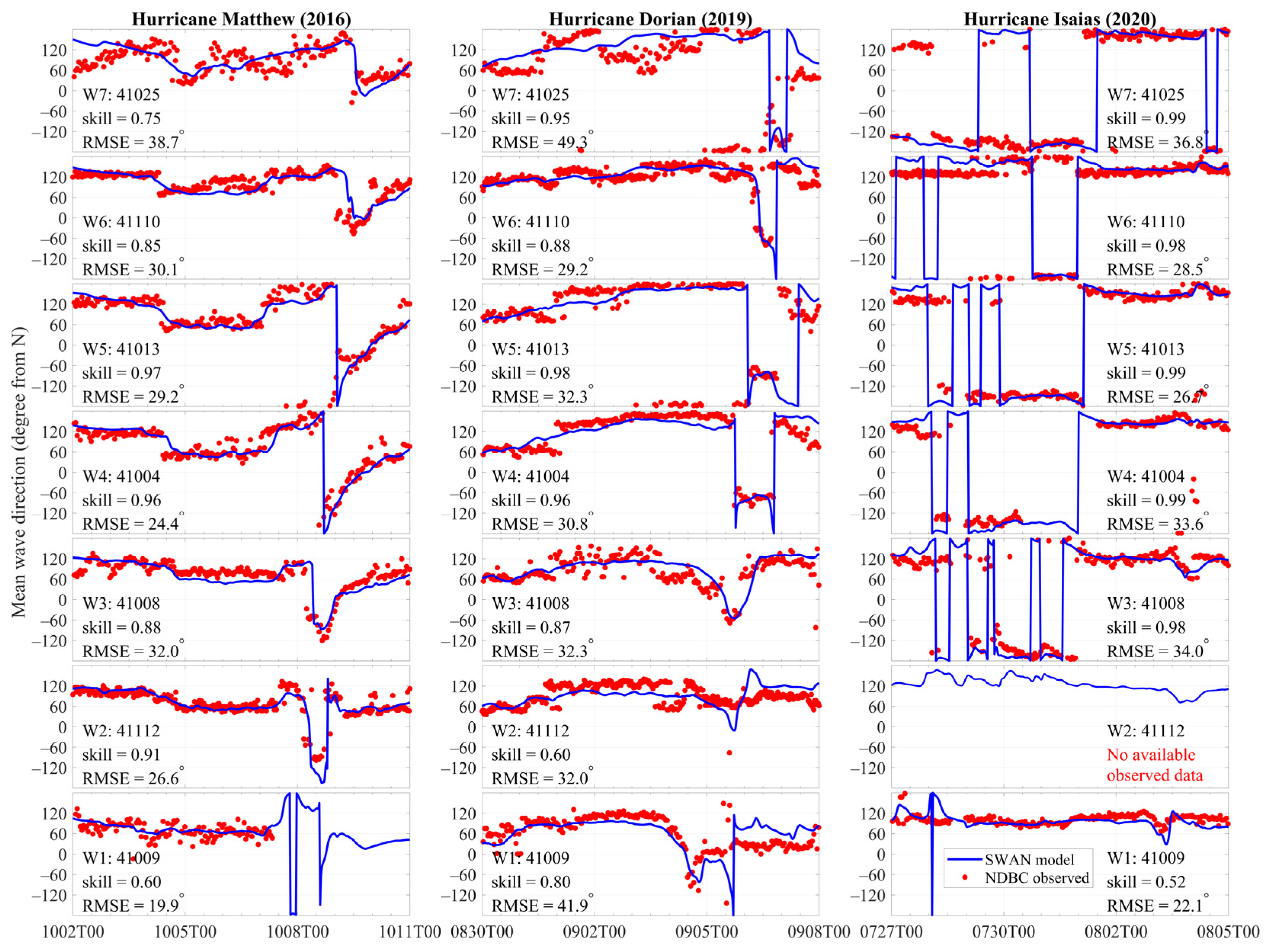
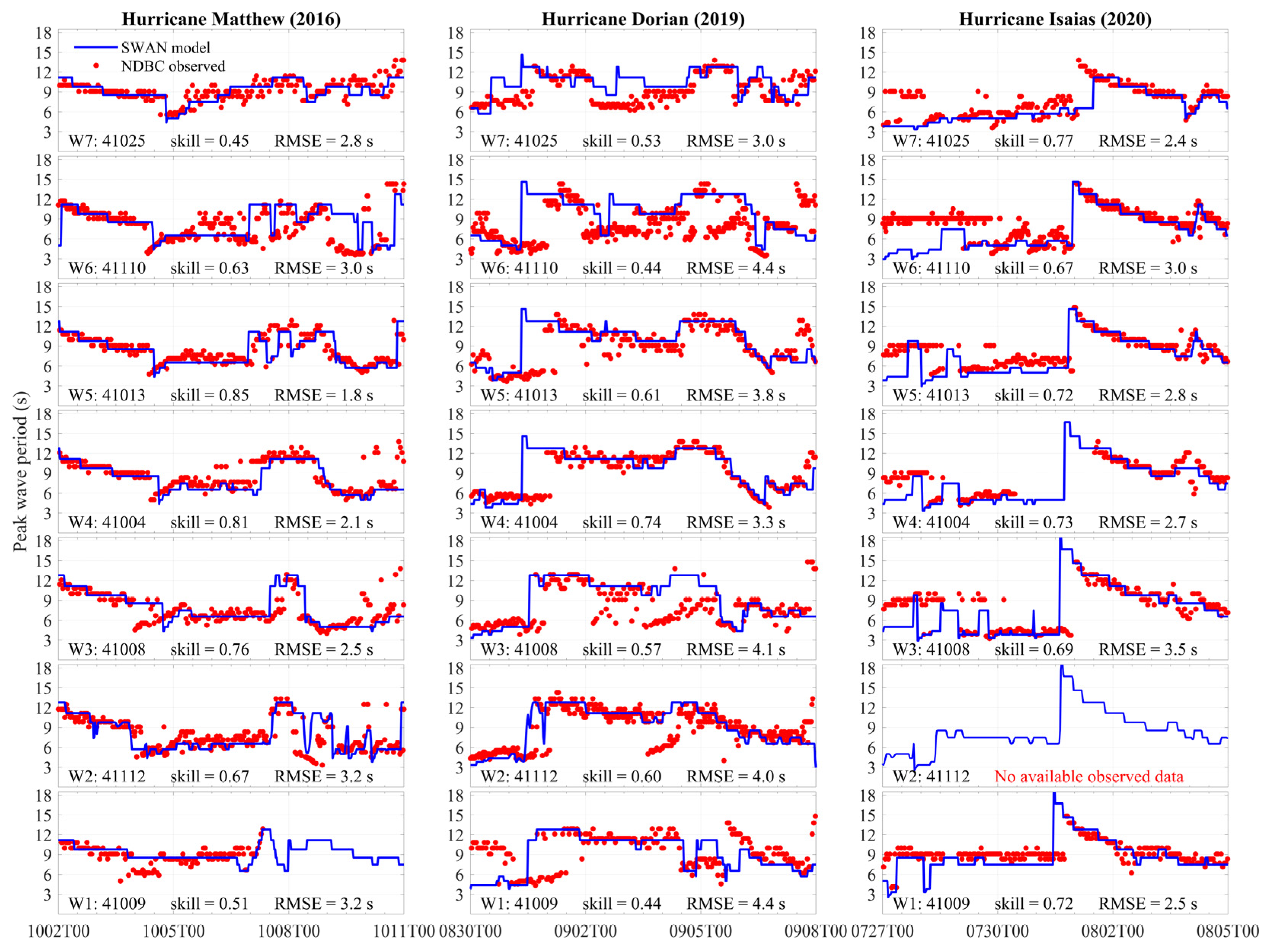
4. Model Verification

Model verification was performed at seven National Data Buoy Center (NDBC) buoys within the SAB. The locations of these NDBC buoys are shown in Figure 2. To quantify the model’s performance, the Willmott model skill (skill) [37] and the root-mean-square error (RMSE) of the three statistical bulk wave parameters (zero-moment wave height, mean wave direction, and peak wave period) were analyzed (

Table 2. Average RMSEs and skills of bulk wave parameters during three hurricanes. $H_{m0}$ is the zero-moment wave height; ${\theta }_M$ is the mean wave direction; and $T_P$ is the peak wave period.

Hurricane	${\mathit{H}}_{\mathit{m}0}$		${\mathit{\theta }}_{\mathit{M}}$		${\mathit{T}}_{\mathit{P}}$
	RMSE (m)	skill	RMSE $(°)$	skill	RMSE (s)	skill
Matthew	0.47	0.96	28.7	0.85	2.66	0.67
Dorian	0.43	0.97	35.4	0.86	3.86	0.56
Isaias	0.42	0.92	30.3	0.90	2.82	0.72
Overall	0.44	0.95	31.5	0.87	3.11	0.65

). The skill was calculated using the formula from ref. [37], as shown in Equation (1). While skill = 1.0 represented a perfect agreement between two datasets, we defined skill = 0.8 as the criterion for good results. The use of the dimensionless skill allowed us to compare model’s performance not only between different stations but among various parameters in different units.

$$skill=1-\frac{{\sum }_1^N{\left|X_{model}-X_{obs}\right|}^2}{{\sum }_1^N{\left(\left|X_{model}-\stackrel{-}{X_{obs}}\right|+\left|X_{obs}-\stackrel{-}{X_{obs}}\right|\right)}^2}$$

(1)

where $X_{model}$ is the model data; $X_{obs}$ is the observed data; $\stackrel{-}{X_{obs}}$ is the averaged value of observed data; and $N$ is the total amount of observations.

The increase in the RMSE represented a decrease in computational accuracy, whereas the increase in skill indicated better model’s performance. RMSEs and skills of zero-moment wave heights, $H_{m0}$, (RMSE $\le$ 0.5 m and skill $\ge$ 0.90), and mean wave direction, ${\theta }_M$, (RMSE $\le$ 40 degrees and skill $\ge$ 0.85) showed good performance.

The relatively high skills of $H_{m0}$ and ${\theta }_M$ indicated that the total wave energy and its mean direction were well reproduced. The comparison between measurements and numerical results of peak wave periods, $T_P$, (RMSE = 3.11 s and skill = 0.65) indicated a larger discrepancy in the frequency width and the dominant wave frequency between observations and simulations. Both indicators during Hurricane Dorian for $T_P$ (RMSE = 3.86 s and skill = 0.56) showed relatively unsatisfactory results compared to the other two hurricanes (Table 2 and Figure A1, Figure A2 and Figure A3 in Appendix A).

5. Wave Spectrogram and Directional Wave Spectrum Evolution

In this section, we compared the existing formulas to separate the sea and swell waves and we analyzed the evolution of the measured frequency–time spectrograms and directional wave spectrum and their dependency with the TC characteristics. Here, five buoys (i.e., NDBC 41009, 41008, 41004, 41013, and 41025) were analyzed, because the other two buoys (i.e., NDBC 41112 and 41110) did not have available observed spectral data. We specifically evaluated the performance of COAWST by comparing measured and model wave spectrograms and directional wave spectrum at NDBC buoy 41008 during these three historical TCs, as the results at this buoy showed the typical pattern of our findings.

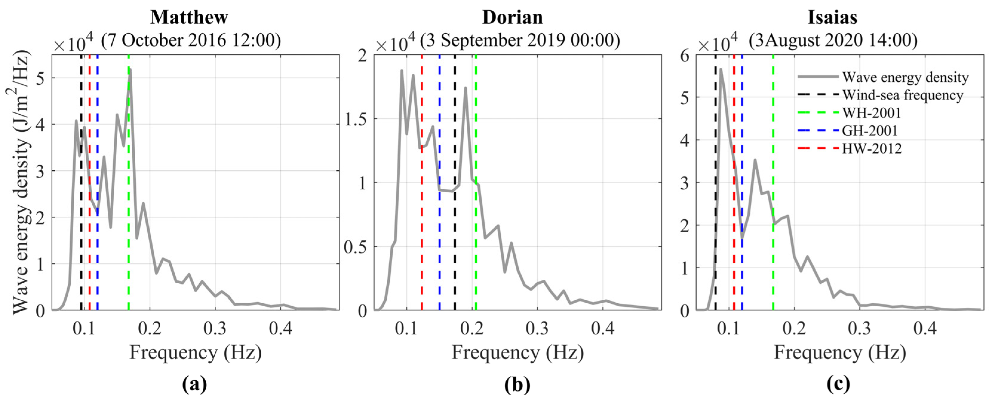
5.1. Sea–Swell Seperation Frequency

The wind-sea peak frequency, $f_{pw}$, was defined as the lowest frequency that the waves can receive energy from the local wind and is given by Equation (2) [7,14].

$$f_{pw}=\frac{g}{2\pi \beta U_{10}}$$

(2)

where $g$ is the gravitational acceleration (${\mathrm{m}}^2{\mathrm{s}}^{-1}$); $U_{10}$ is the wind speed at 10 m above the mean sea level ($\mathrm{m}{\mathrm{s}}^{-1}$); and $\beta$ is a factor set to 1.2 to obtain the approximate wind speed at mean sea level [9,14]. This $f_{pw}$ is referred to as wave age = 0.83 with $\beta =1.2$, which was the sea–swell separation frequency proposed by ref. [5].

We compared the empirical formulas proposed by refs. [7,8,10] for determining the wind-sea–swell separation frequency, $f_S$. In this comparison, the $f_{pw}$ in Equation (2) served as one of the criteria to determine the performance of these empirical formulas. According to refs. [7,10], $f_S$ depended on the peak frequency ($f_{m0}$) of the wave steepness function ($\xi$) shown in Equation (3), which was independent of the wind speed.

$$\xi \left(f\right)=\frac{8\pi m_2\left(f\right)}{g\sqrt{m_0\left(f\right)}}$$

(3)

where $m_0$ and $m_2$ represented the zeroth and the second moments of the wave spectrum, respectively. Ref. [7] defined the sea–swell separation frequency as Equation (4).

$$f_{S-WH2001}=4.112{f_{m0}}^{1.746}$$

(4)

where $f_{m0}$ is the peak frequency of Equation (3).

By considering the Pierson–Moskowitz fully developed wind-sea spectrum [38], ref. [10] improved the wave steepness method of ref. [39] and proposed another sea–swell separation method. NDBC (https://www.ndbc.noaa.gov/faq/windsea.shtml; accessed on 31 March 2023) also used the technique proposed by ref. [10] for sea–swell separation. According to ref. [38], the regime corresponded to swell-dominant conditions when the phase celerity of the peak wave ($C_P$) was larger than 1.25 times the instantaneous local wind speed (i.e., $C_P\ge 1.25U_{10}$). The peak frequency of the Pierson–Moskowitz spectrum was defined as $f_{PM}=1.25/U_{10}$. Ref. [10] considered both wind and wave conditions, and empirically defined the sea–swell separation frequency as Equation (5).

$$f_{S-GH2001}=\mathrm{m}\mathrm{a}\mathrm{x}\left(0.75f_{m0},\hspace{1em}0.90f_{PM}\right)$$

(5)

Ref. [8] used the spectrum integration function (Equation (6)) to smooth down the spikiness of an observed wave energy spectrum. While the method of ref. [7] was documented to place $f_S$ higher than $f_{pw}$ unexpectedly [40], ref. [8] attempted to derive a more accurate $f_S$ without external information (e.g., wind speed). Ref. [8] then proposed an empirical polynomial function for $f_S$ depending on the peak frequency of $I_1$, as shown in Equation (7).

$$I_1\left(f\right)=\frac{m_1\left(f\right)}{\sqrt{m_{-1}\left(f\right)}}=\frac{{\int }_f^{f_u}{f}^{\prime }S\left(f^{\prime }\right)d{f}^{\prime }}{\sqrt{{\int }_f^{f_u}S\left(f^{\prime }\right)/f^{\prime }d{f}^{\prime }}}$$

(6)

$$f_{S-HW2012}=24.2084{f_{m1}}^3-9.2021{f_{m1}}^2+1.8906f_{m1}-0.04286$$

(7)

where $f_u$ is the maximum limit of frequency; $f_{m1}$ is the peak frequency of $I_1\left(f\right)$.

The formulas of refs. [7,8,10] were applied to the wave frequency spectrum at NDBC buoy 41008 during the three historical hurricanes at the timing when a bi-modal wave system was observed (Figure 3). These wave frequency spectra were derived by integrating the wave energy density over the directional space (Equation (8)).

$$S={\int }_0^{360}Ed\theta$$

(8)

where $E$ is the wave energy density ($\mathrm{J}{\mathrm{m}}^{-2}{\mathrm{H}\mathrm{z}}^{-1}{\mathrm{d}\mathrm{e}\mathrm{g}}^{-1}$) and $\mathrm{S}$ is the spectrum energy integrated with respect to the direction ($\mathrm{J}{\mathrm{m}}^{-2}{\mathrm{H}\mathrm{z}}^{-1}$), which is a function of frequency.

In principle, $f_S$ should be lower than $f_{pw}$, since $f_{pw}$ represented the lowest wave frequency that can receive energy from the local wind [8,14]. Additionally, $f_S$ should indicate the frequency of the deeper trough in the frequency spectra, especially when an identifiable bi-modal wave system was observed. These two criteria were used to determine the performance of the considered formulas. We calculated the percentages of the time when $f_S\le f_{pw}$ and $f_S$ lied at local troughs during the three hurricanes (

Table 3. Performance of the formulas to separate sea–swell frequencies at the NDBC buoy 41008 during the three TCs.

	WH–2001	GH–2001	HW–2012
$f_S\le f_{pw}$	32–40%	63–94%	74–91%
$f_S$ lied at local trough	24–32%	20–28%	23–32%

Note that WH–2001 denotes Wang and Hwang (2001) [7]; GH–2001 denotes Gilhousen and Hervey (2001) [10]; and HW–2012 denotes Hwang et al. (2012) [8].

). Higher model’s performance was indicated by higher time percentages, in which $f_S$ lied at local troughs and $f_S\le f_{pw}$.

The WH–2001 gave the lowest percentages among the three formulas, which indicated a less ideal performance for the wind-sea–swell separation frequency. This is consistent with the concern that was documented by ref. [40]. While GH–2001 and HW–2012 gave similar percentages on the $f_S$ lying at local troughs, GH–2001 predicted the $f_S$ at deeper troughs (Figure 3). Thus, hereafter, we used the formula proposed by GH–2001 for the sea–swell separation frequency, $f_S$.

5.2. Wave Spectrogram Behavior

The 2-dimensional wave spectrogram (frequency–time spectrogram) was composed of wave frequency spectra derived from Equation (8) throughout the time series and is shown in Figure 4.

5.2.1. Wave Evolution Phases Associated with the TCs

Phase 1 represents the stage when the wave energy from the TC has not yet approached the buoy. Within phase 1, $H_{m0}$ was generally smaller than 2.0 m. The peak wave frequency was usually higher than 0.2 Hz ($T_P$ < 5.0 s), and the averaged $f_S$ within this phase was generally higher than in the other four phases. The division between phases 1 and 2 is defined by either the first intersection point of $f_S$ and $f_P$ or an abrupt drop of $f_P$. As the remotely TC-generated swell arrived and became the dominant wave component, $f_P$ (red dots in Figure 4a) dropped from > 0.2 Hz to < 0.15 Hz. The normalized distance ($d/R_{max}$; the instantaneous distance to the TC center divided by the instantaneous radius of maximum wind) within phase 2 usually ranged from 8 to 40 during the three historical hurricanes at the considered buoys.

As the TCs approached the buoy, $d/R_{max}$ decreased gradually, and the locally generated wind induced by the outer bands of the TC started to impact the area at the end of phase 2. This was observed through the abrupt increase in $f_P$ (i.e., Dorian) or the gradual decrease in $f_S$ (i.e., Isaias). The beginning of phase 3 is defined when $d/R_{max}\le$ 8.0, following the definition of the near-TC wave field [5]. We did not consider the criterion of $V_{max}\ge$ 33 $\mathrm{m}{\mathrm{s}}^{-1}$ because the wind speed during Isaias did not always reach this level throughout the event. Phase 3 is characterized by a relatively low $f_S$ ($\le$0.15 Hz). The peak energy density increased from ${10}^5$ to ${10}^6$ $\mathrm{J}{\mathrm{m}}^{-2}{\mathrm{H}\mathrm{z}}^{-1}$ (10–100 times of that within phase 2). Within this phase, $H_{m0}$ surged rapidly to its maximum value (Figure A1). The timing when the TC is at its shortest distance to the buoy was defined as the division between phases 3 and 4. Either a sudden increase in $f_S$ (when the buoy was within the TC eye area where the wind speed was extremely low) or the minimum $f_S$ (where the wind speed was extremely high) occurred at this point. While most frequencies can receive energy from the local wind, the energy of low frequencies corresponds to the swell generated by the TC earlier. The division between phases 4 and 5 was determined when $d/R_{max}>$ 8.0 as the TC traveled away from the buoy. Although the buoy was no longer under the direct impact of TC wind waves, the swell generated by the TC propagated to the buoy, keeping $f_P$ as low as in phase 4. Like phase 1, phase 5 represents the stage when the wave field is not affected by TCs.

5.2.2. Phase D (Disturbance): Dominance of Northeasterly Wind by a Continental Cold High during Matthew

The wave spectrograms during Matthew showed an additional phase existing prior to phase 3, which is defined as phase D (disturbance) in the present study. $f_S$ became lower than $f_P$ when Hurricane Matthew was far offshore. At the beginning of this phase, $f_P$ rose instantly and then decreased gradually. Due to its distinctive characteristics and absence during hurricanes Dorian and Isaias, this phase was separated from the other five phases associated with the hurricane wind waves.

5.2.3. SWAN Model’s Performance for Wave Energy Spectrogram

On average, the energy density around $f_P$ (0.06 Hz–0.15 Hz) was underestimated by 10–25% within phase 1, and by 25–50% within phase 2 (blue in Figure 4b). The energy density of frequencies $<$ 0.06 Hz and 0.15 Hz $\le$ frequencies $<$ 0.25 Hz (red within phase 1 and/or the beginning of phase 2 in Figure 4b) were generally overestimated by SWAN. Consequently, the frequency spreading of energy density higher than 1000 $\mathrm{J}{\mathrm{m}}^{-2}{\mathrm{H}\mathrm{z}}^{-1}$ (3.0 in the logarithmic scale) can be overestimated by SWAN by up to three times of the observed data (e.g., phase 1 during Matthew and the beginning of phase 2 during Dorian). In contrast, the energy density of 0.06 Hz–0.15 Hz was underestimated, which eventually led to an overall underestimated $H_{m0}$ within phase 2. According to the corresponding $f_S$, this indicated that the swell frequency spreading was overestimated and the total swell energy was underestimated.

From the end of phase 2 to the beginning of phase 3, where the energy density increased by at least one order of magnitude (Figure 4a), the wave energy was underestimated during all three TCs. This was also reflected in the underestimation of $H_{m0}$ (Figure A1 in Appendix A). Within phase 4, the model peak energy generally shifted toward the lower frequency (swell) compared to the observations. The energy density of lower frequencies ($<$0.15 Hz) was overestimated by $<$5%, whereas the energy density at higher frequencies (0.15 Hz–0.25 Hz) was underestimated by $<$25%. This pattern was observed at NDBC buoys 41008, 41004, 41013, and 41025 during the three hurricanes. Unlike the overestimation of frequency spreading observed within phase 1, this indicated the underestimation of $f_P$ and the swell energy level.

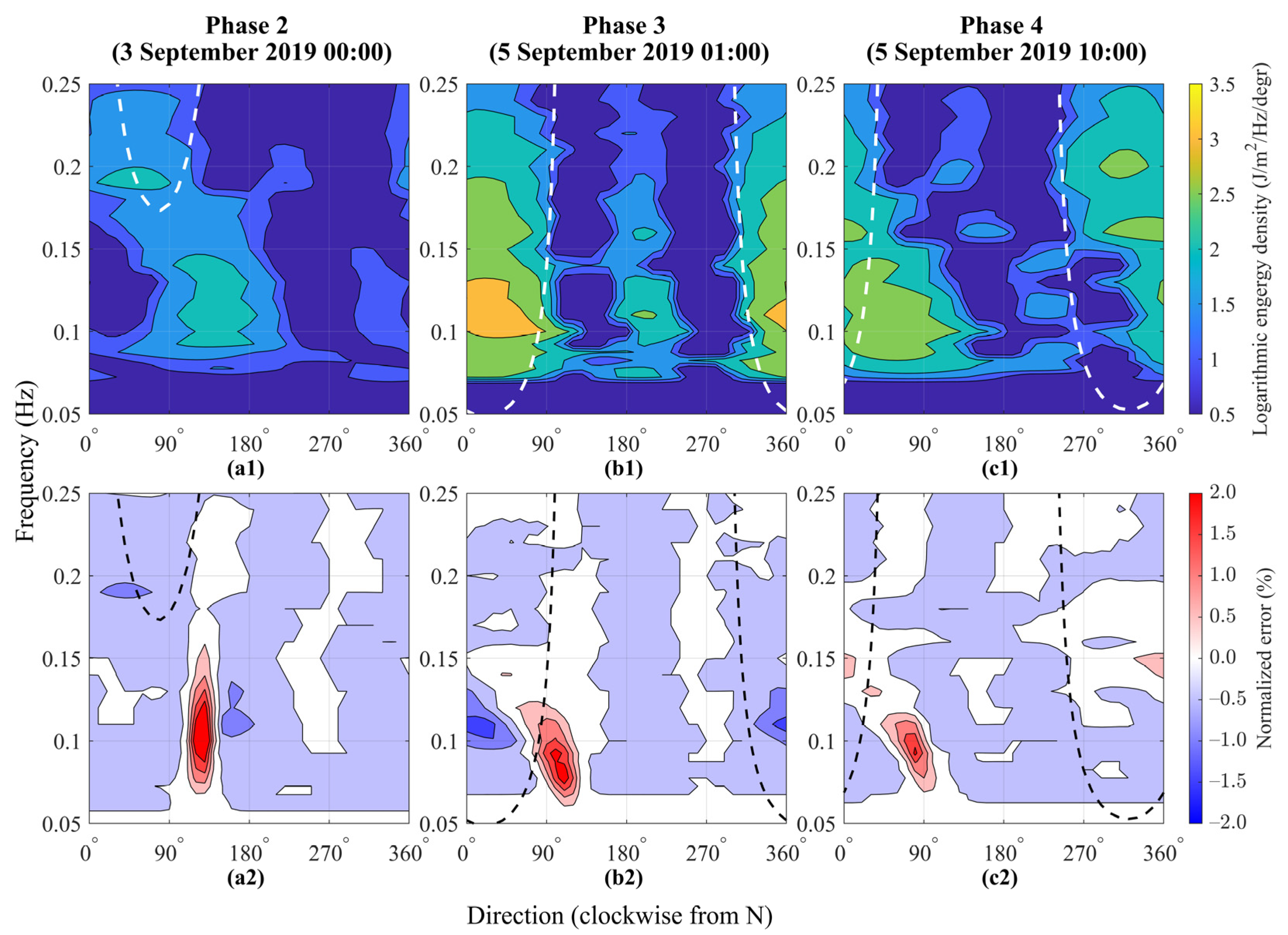
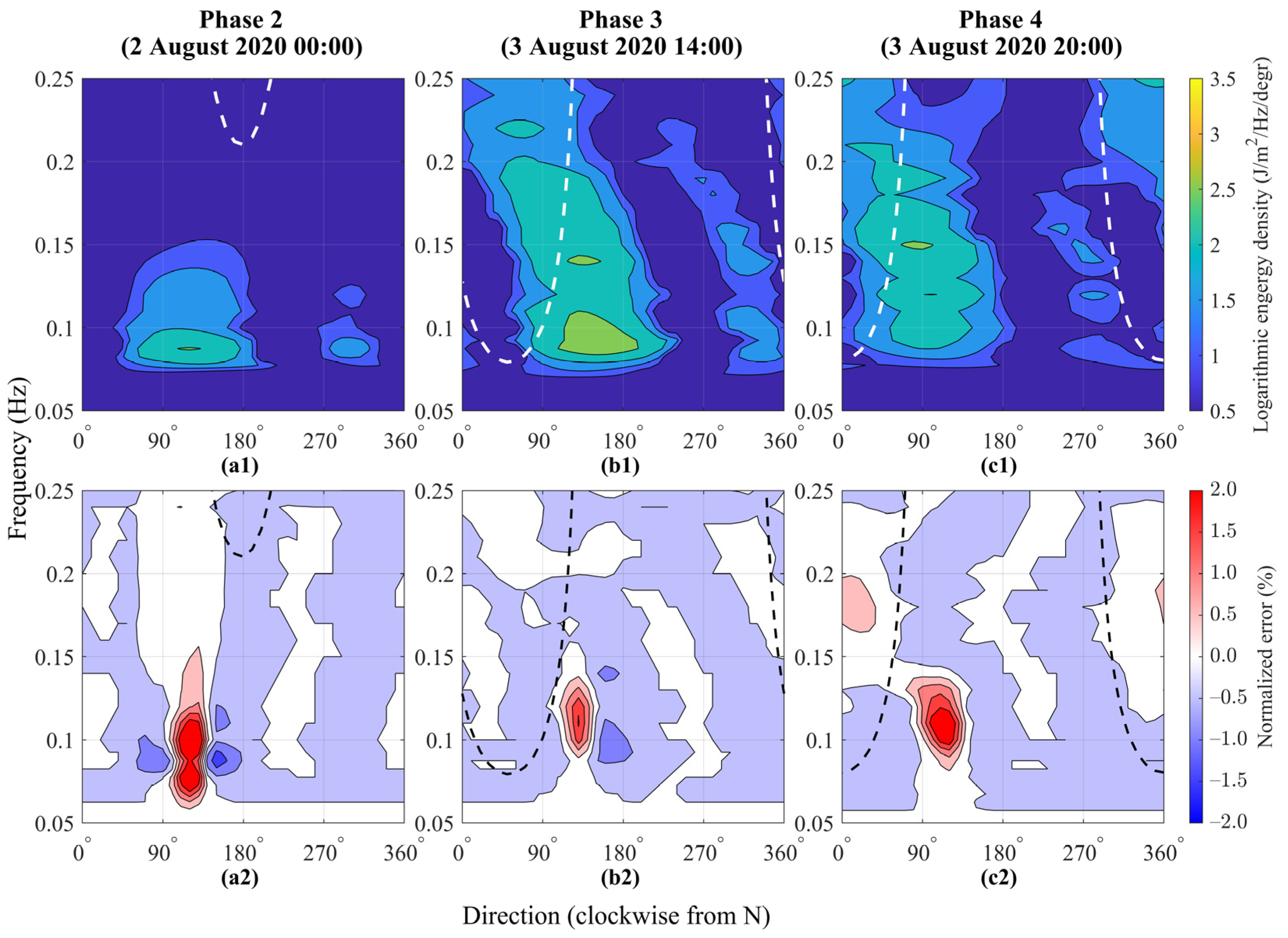
5.3. Directional Wave Spectra

The five phases identified in the previous section showed different structures in the wave frequency spectrograms. While the wave spectrogram represents the variation of energy density with respect to frequency and time, the directional wave spectra show how energy density is distributed with respect to frequency and direction instantaneously. However, the observed wave energy spectra can have various signal noises, and the boundaries between wave systems can be hard to verify. Following ref. [27], we employed the 2-dimensional convolution operation to carry out the weighted averages of the adjacent peaks in directional wave spectra extracted from different phases (Figure 5, Figure 6 and Figure 7). The convolution operation served as an image smoother filter here, which made different wave systems more identifiable. We used the criteria based on the wave age ($U_{10}·\cos \left({\theta }_M-{\theta }_W\right)/C_p\le$ 0.83; ${\theta }_W$ was the wind direction.) suggested by ref. [5] to separate the sea and swell components of the directional wave spectra. The resulting parabola that separated the sea and swell waves was depicted together with the directional wave spectra (Figure 5, Figure 6 and Figure 7). The regime within the parabola corresponds to sea waves, whereas the energy outside the parabola corresponds to swell. The instantaneous local wind direction is indicated by the peak of the parabola.

The directional wave spectrum of phase D during Hurricane Matthew (Figure 5(a1)) showed a bi-modal wave system. The wave mode associated with the local wind (overlapped with the wave age parabola) came from the east–northeast. The other mode came from the west–southwest. Both modes had peak energy around a wave frequency of 0.15 Hz–0.20 Hz, and the angle difference between the two modes was approximately 180$°$. A similar pattern can be found in phase 3 during Matthew (Figure 5(b1)). The main difference was that the energy levels during phase 3 were higher than in phase D. As Hurricane Matthew moved forward and passed over the buoy, the wind direction (the peak of the white parabola) changed remarkably in phase 4. Meanwhile, the peak energy within phase 4 shifted to higher frequencies (i.e., 0.15 Hz–0.20 Hz) compared to phase 3.

In regard to the computational discrepancy during phases 3 and 4, the overestimation at the direction with the largest overestimation (120$°$ in Figure 5(b2,c2)) and the underestimation around the peak direction indicated an underestimation of directional spreading (Figure 5(b2,c2)). The swell energy (i.e., 0.05 Hz–0.15 Hz) within a directional bin of approximately 60$°$ was overestimated. While this swell energy can still receive energy from the local wind (i.e., inside the young wave age parabola) during phase 3, this swell energy was completely remotely generated and propagated toward the buoy during phase 4 as the storm traveled away. It is worth noting that the most significant underestimated energy throughout the three snapshots was observed within the window of 0.12 Hz–0.18 Hz and 270$°$–360$°$. According to the instantaneous TC location and the wave age parabola, this underestimated wave energy was the wind-sea generated by Hurricane Matthew. Additionally, when there was a wave system coming from the east, i.e., 90$°$, another wave system with a 180$°$ difference, i.e., 270$°$, was observed (see Figure 5(a1,b1)). These two wave systems had similar peak frequencies lower than 0.18 Hz. It is also worth noting that the energy density of this wave system coming from 270$°$ was not reproduced by the SWAN model and resulted in an underestimated regime (see Figure 5(a2,b2)).

The direction of the SAB shoreline near NDBC buoy 41008 is approximately 27$°$ clockwise to the north. The distance between NDBC buoy 41008 and the shore is approximately 33 km, and its water depth is 16 m. Considering the direction, frequency, and shoreline characteristics, this wave system propagating from 270$°$ can thus be identified as the reflected waves from the coast associated with TC-induced swells. In the SWAN model setup, we did not consider wave reflection, which explains the underestimation of energy in this regime.

The young wave age parabola of the directional wave spectrum snapshot within phase 2 during Dorian covered a much smaller area compared to phases 3 and 4, indicating a much lower local wind speed (see Figure 6(a1–c1)). Most of the wave energy belonged to the swell within phase 2 during Dorian, while there was a stronger local wind wave system during phases 3 and 4. The directional wave spectrum extracted from phase 3 during Hurricane Dorian had a similar structure to that of Hurricane Matthew: (1) a multi-modal wave system lied within the parabola of young wave age; (2) a reflected wave system came from the direction with a 180$°$ difference with a peak frequency lower than 0.15 Hz. Within phase 4, the wind-sea peak frequency exceeded 0.15 Hz, and the wind-sea direction changed to around 330$°$ as the storm moved northeastward. The swell coming from 60$°$ was thus generated by the storm and propagated back to the buoy (see Figure 6(c1)).

Compared to Hurricane Matthew, the discrepancy in swell energy prior to phase 3 was more evident during Dorian (Figure 6(a2)). Compared to the NDBC-observed spectrum, the model swell energy was concentrated within a narrower directional band. This underestimated directional spreading of swell energy existed throughout the three phases during Dorian (Figure 6(a2–c2)).

Compared to hurricanes Matthew and Dorian, the local wind speed prior to phase 3 was weaker during Isaias (see the smaller parabola area in Figure 7(a1)). While Matthew and Dorian were major hurricanes according to their intensity, Isaias was a category 1 hurricane at its peak. Additionally, Isaias had the fastest translation speed within the SAB (see Table 1). These differences led to a different directional wave spectral structure during Isaias. Within phase 2, a main wave system within the window of 0.07 Hz–0.18 Hz and 45$°$–180$°$ was observed (Figure 7(a1)). This wave system belonged to the swell according to its frequency distribution. This swell associated with distant Isaias (i.e., $d/R_{max}\cong$ 20.0) had a higher peak energy compared to phase 2 of Hurricane Dorian (Figure 6(a1)), despite Isaias’s lower intensity. The peak frequency of this wave system was lower during Isaias compared to Dorian. The role of the TC translation speed in the generation of this swell is further described in Section 6. Another wave system with similar frequency spreading but a 180$°$ difference in the directional bin was observed. Located outside the young wave age parabola, both wave systems were associated with the swell. While the first wave system from east–southeast denoted the swell generated by Isaias, the second wave system represented the corresponding reflected waves.

The discrepancy between the observations and model results in the swell energy prior to phase 3 during Isaias was the most remarkable among the three historical storms (Figure 7(a2)). While the energy level at the peak direction was overestimated by similar normalized error levels ($\cong$2%), the nearby directional bins experienced a more evident underestimation of the energy density compared to Dorian.

In addition to the underestimation of the reflected wave energy associated with the swell, another common feature was observed through the three hurricanes. This was the overestimation of energy density around the window of 0.07 Hz–0.13 Hz and 75$°$–150$°$ within phases 3 and 4. Although this overestimation area shifted slightly from storm to storm, the directional bin with the highest overestimation was similar from the six snapshots (Figure 5(b2,c2), Figure 6(b2,c2), and Figure 7(b2,c2)).

To further verify the overall model’s performance with respect to time, we calculated the normalized RMSEs of an instantaneous directional wave spectrum during the three hurricanes. We divided the RMSEs of wave energy density by the integrated energy throughout the instantaneous observed directional wave spectra. This normalization eliminates the impact of the total energy density variation on numerical errors. Throughout the five buoys (NDBC 41009, 41008, 41004, 41013, and 41025) during the three hurricanes (i.e., 15 datasets in total), more than half of the peak normalized RMSEs occurred within phases 3 and 4, as the storm passed over the buoys. We applied a TC-referenced coordinate system [13] to analyze wind and wave fields within phases 3 and 4 at NDBC buoy 41008 (Figure 8). The instantaneous $d/R_{max}$ was less than 8.0 within phases 3 and 4, according to the aforementioned definitions. The analyzed buoys were found to lie in the front-left (FL) or front-right (FR) quadrants with respect to the TC’s location and heading direction within phase 3, and transferred to the rear-left (RL) or rear-right (RR) quadrants within phase 4. The wind (gray vectors in Figure 8) and the mean waves (red vectors in Figure 8) showed that the difference between wind and wave directions was relatively small in the FL and FR quadrants, whereas they were in nearly opposite directions in the RL and RR quadrants.

6. Discussion

The five phases identified in the present work were found in other areas and during other TCs as well. Take Typhoons Fanapi (2010) and Megi (2010) for instance. According to the intersections of $f_P$ and $f_{pw}$ at buoys EASI–N during Fanapi and EASI–S Megi [14], phases 2, 3, 4, and 5 can be observed. The durations and the wave energy density within the phases were affected by the relative position of the buoys with respect to the TC eye and the TC properties. The dominant factors in energy distribution varied from phase to phase. The following sections discussed the linkages between the atmospheric conditions, wave dynamics, and numerical modeling performance during the three analyzed TCs.

6.1. Use of Wind-Sea–Swell Seperation Frequencies

This study compared the applicability of the formulas for the wind-sea–swell separation frequency by refs. [7,8,10]. While the formula by ref. [8] has been widely used (e.g., ref. [27]), we found that the formula proposed by ref. [10] had comparable or more ideal performance on the wave spectrum during the considered historical storm events. This implies that the sensitivity and accuracy of various formulas for $f_S$ should be tested before their application. Additionally, the better results of the formula in ref. [10] demonstrated the necessity of considering external data such as wind speed for sea-swell separation when available. While the wind speed is unavailable, the formula from ref. [8] is recommended.

6.2. Effect of Atmospheric Conditions on Wave Spectrograms

The main features of the time–frequency wave spectrogram (Figure 4) and time series of wave heights (Figure A1 in Appendix A) were distinct during Matthew and Dorian, despite their similarities in the maximum wind speeds and radii of maximum wind within the SAB. However, local waves may have been affected by other weather systems. An increase in the local wind speed stemmed from a large pressure gradient due to the continental cold high located around the Gulf of St. Lawrence during Matthew. Within phase D of buoy 41008 during Hurricane Matthew (top panel of Figure 4a and Figure 5(a1)), this system resulted in north-easterly winds along the U.S. East Coast. The larger instantaneous $d/R_{max}$ ($\ge$20), higher $f_P$ ($\ge f_S$), and larger area covered by the young wave age parabola indicated that the increase in $H_{m0}$ observed at this moment was not related to Matthew. The pressure gradient around the same areas during Dorian was not as large as that during Matthew. Consequently, the north-easterly wind around the SAB was relatively weak ($\le$10 $\mathrm{m}{\mathrm{s}}^{-1}$) at buoy 41008 within phase 2 during Dorian. Hurricane Isaias formed earlier in the year than the other two hurricanes. In July 2020, the high-pressure center was still in the ocean. The pressure gradient around the SAB was even weaker compared to that during Dorian.

Among the five buoys (NDBC 41009, 41008, 41004, 41013, and 41025), only buoys 41008 and 41025 were located on the left-hand side of Matthew’s track. During Dorian, buoy 41008 was located on the left-hand side of the TC track. This indicates that these buoys transitioned from the FL quadrant to the RL quadrant as the storms passed over. As Matthew passed over buoys 41008 and 41025 and Dorian passed over buoy 41008, the TC heading directions were directed toward NNE and NE, respectively. An eastward component of the TC translation speed increased the total wind velocities in the offshore direction as the buoys transitioned from the FL to the RL quadrants.

6.3. Effect of TC Translation Speed on Wave Energy Distribution

Most features of the wave spectrogram were found to be directly related to the instantaneous TC characteristics. Hurricanes Matthew and Isaias traveled with faster TC translation speeds (6.2 $\mathrm{m}{\mathrm{s}}^{-1}$ and 6.3 $\mathrm{m}{\mathrm{s}}^{-1}$) on average within the SAB compared to Dorian (3.3 $\mathrm{m}{\mathrm{s}}^{-1}$). Ref. [41] stated that the mean translation speeds varied between 4.2 $\mathrm{m}{\mathrm{s}}^{-1}$ and 6.0 $\mathrm{m}{\mathrm{s}}^{-1}$ for hurricanes of all categories. Dorian propagated with a slow TC translation speed, which was lower than the global average (4.8 $\mathrm{m}{\mathrm{s}}^{-1}$) for its category [41]. The smaller TC translation speed of Dorian within the SAB allowed its swell to dominate the wave field for longer before the TC’s approach and resulted in a longer, integrated duration of phases 2, 3, and 4 compared to Matthew and Isaias (Figure 4).

Refs. [42,43] stated that the wave energy and the wavelength increased with the TC translation speed until the wind speed reached 13 $\mathrm{m}{\mathrm{s}}^{-1}$ because of the prolonged effective wind fetch. The averaged TC translation speeds of Dorian (3.3 $\mathrm{m}{\mathrm{s}}^{-1}$) and Isaias (6.3 $\mathrm{m}{\mathrm{s}}^{-1}$) were very different within the SAB (Table 1). Consequently, the peak wave frequency ($f_P$= 0.06 Hz, $T_P$= 16 s) in phase 2 during Isaias was lower than that of Dorian ($f_P$ = 0.08 Hz, $T_P$ = 13 s) (Figure 4, Figure 6 and Figure 7). This is consistent with the findings of ref. [43]. In addition to the difference in the peak wave frequency, we found that the translation speed may have impacted the model’s performance of frequency spreading. Within phase 2 during Isaias, the colormap showed a red–blue–red pattern across frequencies 0.05 Hz to 0.10 Hz at the five considered buoys (NDBC 41009, 41008, 41004, 41013, and 41025), which was not observed during Dorian (Figure 4). This indicates that the frequency spreading around $f_P$ was overestimated more during Isaias than Dorian within the swell-dominant phase (phase 2). The results revealed that the current model settings may not well reproduce the peak of the frequency spectrum with faster TC translation speeds and indicated that the energy of $f_P$ built less compared to the observations.

6.4. Formation of Multi-Modal Directional Wave Spectra

Waves coming from various directional bins and/or affiliated with various frequencies with comparable energy resulted in the formation of multi-modal spectra. This can be caused by other weather events or different wave types. For instance, the wave frequency spectrogram at the beginning of phase D during Matthew at NDBC buoy 41008 was dominated by a tri-modal wave system. One of the modes was primarily contributed by the north-easterly wind waves generated locally. The energy density of this mode was mainly concentrated within the window of 0.15 Hz–0.25 Hz and 0$°$–120$°$. Another mode was primarily composed of the remotely generated swell, mainly concentrating within the window of 0.07 Hz–0.15 Hz and 0$°$–120$°$. This mode hardly received energy from the local wind because of its faster phase celerity. The last mode was concentrated at the same frequencies as the swell mode but from nearly the opposite direction. This mode corresponds to the reflected long waves (associated with the swell) from the coast and consisted of 4–8% integrated wave energy of the instantaneous spectrum.

As the hurricane approached and passed over specific buoys, waves generated by the local wind varied rapidly with the wind direction. Meanwhile, the direction of swells generated remotely did not change much. Consequently, the wave energy of higher frequencies (locally generated wind waves) came from different directions, and the wave of lower frequencies (swells) concentrated within a narrower directional band. This led to the formation of multi-modal spectra.

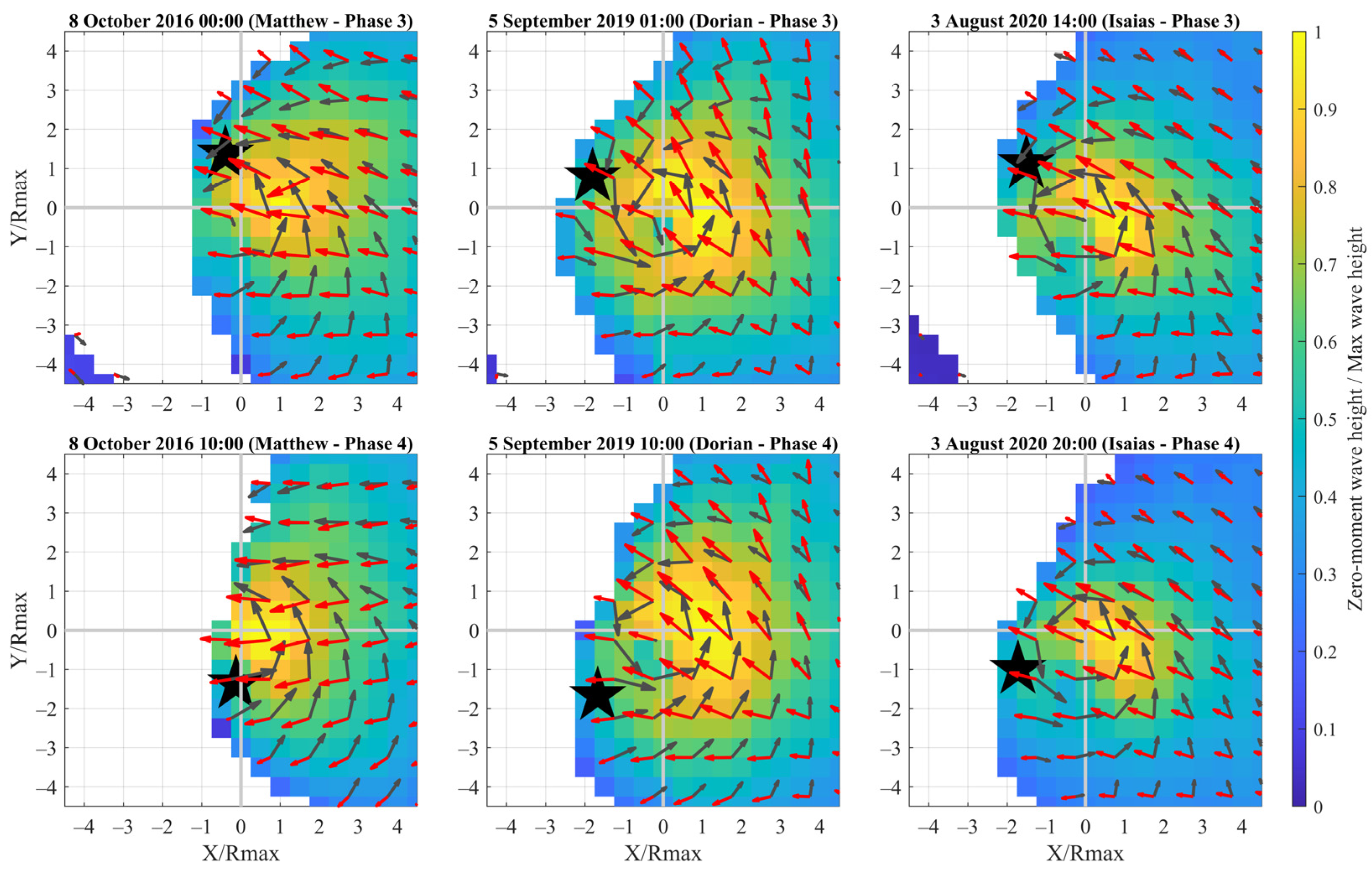
6.5. Model’s Performance on Wave Energy Distribution

The normalized RMSEs of the directional wave energy spectrum at each buoy within phases 3 and 4 were used to determine the effects of each TC property on the performance of a model’s energy distribution. This criterion ensured that the wave field was under the direct impact of the TCs. Five buoys (NDBC 41009, 41008, 41004, 41013, and 41025) during three TCs were considered in the wave spectral analysis (i.e., 15 scenarios in total). The normalized RMSEs of directional energy density reached the peak at a value of 0.2–0.6% within phases 3 and 4 in eight scenarios. The corresponding energy density of the locally generated wind waves was underestimated, which may be related to the insufficient time for wind waves development in the model due to rapid changes in the wind’s direction. On the other hand, the energy density of the swell was usually overestimated by the model in the meanwhile. We calculated the correlation coefficients ($R$) and p values ($P$) between four instantaneous TC characteristics and the normalized RMSEs. Higher absolute values of correlation coefficients and lower p values indicate a higher correlation between the parameters. The normalized RMSEs had a higher correlation with instantaneous $V_{max}$ and $P_{min}$ (

Table 4. Correlation coefficients and p values between four TC properties and the relative computational error of wave energy spectrum when $d/R_{max}\le$ 8.0 and $V_{max}\ge$ 33 $\mathrm{m}{\mathrm{s}}^{-1}$ at five NDBC buoys (NDBC 41009, 41008, 41004, 41013, and 41025) during three hurricanes.

TC Properties	${\mathit{V}}_{\mathit{t}}$	${\mathit{V}}_{\mathit{m}\mathit{a}\mathit{x}}$	${\mathit{P}}_{\mathit{m}\mathit{i}\mathit{n}}$	${\mathit{R}}_{\mathit{m}\mathit{a}\mathit{x}}$
Correlation coefficient (R)	$-$0.10	0.13	$-$0.13	0.10
p values (p)	0.041	0.009	0.007	0.052

). Results indicate that a larger computational error on wave energy distribution is expected if a TC has a lower $P_{min}$ and/or a larger $V_{max}$ within the near-TC wave field.

Ref. [16] documented that the DIA for quadruplet non-linear wave–wave interactions may lead to an overprediction of the wave energy below $f_P$. This was consistent with what we observed, particularly within phase 4 at buoys 41008, 41004, and 41013. Ref. [16] stated that another approach proposed by ref. [44] may improve the drawback of overestimated frequency spreading. However, ref. [16] also mentioned that DIA generally had a better performance on the integral wave height than the approach of ref. [44]. We found that this overprediction of energy below $f_P$ within phase 4 was much more obvious during Dorian, while a slight overestimation of energy was observed during Matthew and Isaias. As documented by ref. [16] and the scientific and technical documentation of SWAN, DIA had a lower performance on relatively long-crest waves (swell). Phase 2 was revealed to be swell-dominant, and Isaias was found to have higher pre-storm swells due to its faster translation speed.

The numerical discrepancy in wave frequency spectrograms and directional wave spectra showed that our modeling system underestimated the directional spreading and overestimated the frequency spreading. The model’s performance on energy distribution was found to depend on the TC characteristics, according to the results. The swell energy (frequencies < 0.15 Hz) was usually overestimated in the modeling system, while the locally generated wind wave energy was generally underestimated. This might result in an underestimation of the wave height within phase 3 (Figure A1 in Appendix A). Phase 3 was when the maximum normalized RMSEs of the directional wave spectra usually occurred.

Overall, as stated by the report of the IPCC [4], TC characteristics will change under climate change and global warming on a global scale. The TC intensity and occurrence frequency of stronger storms were projected to increase. The forecasting accuracy of frequency spreading and peak wave energy need further evaluation. The relation between wave dynamics and the model’s performance within different phases under different TC scenarios has been pointed out. An increase in the TC translation speed within phase 2 may lead to a more severe computational discrepancy in the swell energy and directional spreading.

7. Conclusions

Three formulas for wind-sea–swell separation frequencies were compared, and the suggested formula based on the principles of relevant studies and NDBC-observed data was presented. Our results indicated that the method considering both wind and wave data in the calculation of wind-sea–swell separation frequencies, captured the deeper local trough in the wave frequency spectrum, and provided better results. We also determined the model’s performance on statistical wave bulk parameters, wave energy distributions, and wave energy evolution within the SAB during three historical hurricanes. The results showed that the behaviors of $H_{m0}$ and ${\theta }_M$ were well captured by the model. We analyzed the wave frequency spectrogram and directional wave spectrum at various buoys during the historical hurricanes to understand the frequency spreading, directional spreading, and energy evolution under these severe weather events. Five phases were observed and defined based on the normalized distance to the TC eye, the peak wave frequency, and the wind-sea–swell separation frequency. These five phases can be used to interpret different stages of wave-field evolution during TCs.

The characteristics and model’s performance of directional wave spectra within each phase were also discussed. A multi-modal directional wave spectrum can be observed within the phases when TC-induced spectral components existed, but due to different reasons. The tri-modal system within phase 2 is generally related to the swell generated remotely by TCs and the corresponding waves reflection from the coast. The reflected wave was distinctive in this multi-modal system, and it consisted of 4–8% in terms of the total wave energy instantaneously. However, this percentage and phenomenon varied from storm to storm. The multi-modal system with three modes was observed within phases 2 and 3. As a TC approached specific buoys, ocean waves received energy from wind in various directions, which resulted in comparable wave energy in various directions. Three wave modes with comparable energy intensities were usually observed from the snapshot of the directional spectrum across phases 2 and 3: the swell, the reflected waves of the swell, and the local wind waves. The existence and intensity of each mode strongly depended on the relative position (i.e., quadrant and normalized distance) to the TC and the instantaneous TC intensity and TC translation speed. The reflected waves associated with the swell were relevant, especially when the swell propagated perpendicularly to the coast. From phases 3 to 4, the wind field experienced a rapid transformation as a TC passed over. Consequently, the swell generated remotely by the TC earlier remained in almost the same direction, while the locally generated wind wave changed its direction significantly. This was generally the moment when the normalized RMSEs of the instantaneous directional wave spectrum reached their maximum within the near-TC wave field. This peak of the normalized RMSEs of energy density was primarily related to two factors. The first was the overestimation of swell, and the second was the rapidly changing wind direction, which the model wind wave did not have sufficient time to develop compared to reality. This study provided an insight into the scenarios (e.g., according to the predicted path, TC translation speed, and TC intensity) in which the forecasted results may not be accurate and has thus paved the way for further improvements.

References

1. Stockdon, H.F.; Holman, R.A.; Howd, P.A.; Sallenger, A.H., Jr. Empirical parameterization of setup, swash, and runup. Coast. Eng. 2006, 53, 573–588. [Google Scholar] [CrossRef]
2. Hsu, C.-E.; Serafin, K.; Yu, X.; Hegermiller, C.A.; Warner, J.C.; Olabarrieta, M. Total water levels along the South Atlantic Bight during three along–shelf propagating tropical cyclones: Relative contributions of storm surge and wave runup. Nat. Hazards Earth Syst. Sci. Discuss (Prepr. Rev.) 2023, 2023, 1–31. [Google Scholar] [CrossRef]
3. National Oceanic and Atmospheric Administration. National Coastal Population Report: Population Trends from 1970 to 2010. NOAA State of the Coast Report Series. 2013. Available online: https://coast.noaa.gov/digitalcoast/training/population-report.html (accessed on 23 May 2023).
4. Masson Delmotte, V.; Zhai, P.; Pirani, A.; Connors, S.L.; Péan, C.; Berger, S.; Caud, N.; Chen, Y.; Goldfarb, L.; Gomis, M.I.; et al. Climate Change 2021: The Physical Science Basis. Contribution of Working Group I to the Sixth Assessment Report of the Intergovernmental Panel on Climate Change. 2021. Available online: https://www.ipcc.ch/report/ar6/wg1/ (accessed on 23 May 2023).
5. Young, I.R. Directional spectra of hurricane wind waves. J. Geophys. Res. Ocean. 2006, 111, C08020. [Google Scholar] [CrossRef]
6. Nair, M.A.; Kumar, V.S.; George, V. Evolution of wave spectra during sea breeze and tropical cyclone. Ocean. Eng. 2021, 219, 108341. [Google Scholar] [CrossRef]
7. Wang, D.W.; Hwang, P.A. An operational method for separating wind sea and swell from ocean wave spectra. J. Atmos. Ocean. Technol. 2001, 18, 2052–2062. [Google Scholar] [CrossRef]
8. Hwang, P.A.; Ocampo Torres, F.J.; Garcia Nava, H. Wind sea and swell separation of 1D wave spectrum by a spectrum integration method. J. Atmos. Ocean. Technol. 2012, 29, 116–128. [Google Scholar] [CrossRef]
9. Potter, H. Swell and the drag coefficient. Ocean. Dyn. 2015, 65, 375–384. [Google Scholar] [CrossRef]
10. Gilhousen, D.B.; Hervey, R. Improved estimates of swell from moored buoys. In Proceedings of the Fourth International Symposium WAVES 2001; ASCE: Alexandria, VA, USA, 2001. Available online: https://ascelibrary.org/doi/pdf/10.1061/40604%28273%2940 (accessed on 23 May 2023).
11. Ewans, K.C.; Bitner Gregersen, E.M.; Soares, C.G. Estimation of wind–sea and swell components in a bimodal sea state. J. Offshore Mech. Arct. Eng. 2006, 128, 265–270. [Google Scholar] [CrossRef]
12. Moon, I.J.; Ginis, I.; Hara, T.; Tolman, H.L.; Wright, C.W.; Walsh, E.J. Numerical simulation of sea surface directional wave spectra under hurricane wind forcing. J. Phys. Oceanogr. 2003, 33, 1680–1706. [Google Scholar] [CrossRef]
13. Esquivel Trava, B.; Ocampo Torres, F.J.; Osuna, P. Spatial structure of directional wave spectra in hurricanes. Ocean. Dyn. 2015, 65, 65–76. [Google Scholar] [CrossRef]
14. Collins, C.O.; Potter, H.; Lund, B.; Tamura, H.; Graber, H.C. Directional wave spectra observed during intense tropical cyclones. J. Geophys. Res. Ocean. 2018, 123, 773–793. [Google Scholar] [CrossRef]
15. Booij, N.; Ris, R.C.; Holthuijsen, L.H. A third–generation wave model for coastal regions—1. Model description and validation. J. Geophys. Res. Ocean. 1999, 104, 7649–7666. [Google Scholar] [CrossRef]
16. Rogers, W.E.; Van Vledder, G.P. Frequency width in predictions of windsea spectra and the role of the nonlinear solver. Ocean. Model. 2013, 70, 52–61. [Google Scholar] [CrossRef]
17. Shchepetkin, A.F.; McWilliams, J.C. The regional oceanic modeling system (ROMS): A split–explicit, free–surface, topography–following–coordinate oceanic model. Ocean. Model. 2005, 9, 347–404. [Google Scholar] [CrossRef]
18. Warner, J.C.; Sherwood, C.R.; Signell, R.P.; Harris, C.K.; Arango, H.G. Development of a 3-dimensional, regional, coupled wave, current, and sediment–transport model. Comput. Geosci. 2008, 34, 1284–1306. [Google Scholar] [CrossRef]
19. Warner, J.C.; Armstrong, B.; He, R.; Zambon, J.B. Development of a Coupled Ocean–Atmosphere–Wave–Sediment Transport (COAWST) Modeling System. Ocean. Model. 2010, 35, 230–244. [Google Scholar] [CrossRef]
20. Hsu, C.-E.; Hsiao, S.-C.; Hsu, J.-T. Parametric analyses of wave–induced nearshore current system. J. Coast. Res. 2017, 33, 795–801. [Google Scholar] [CrossRef]
21. Thomas, A.; Dietrich, J.C.; Asher, T.G.; Bell, M.; Blanton, B.O.; Copeland, J.H.; Cox, A.T.; Dawson, C.N.; Fleming, J.G.; Luettich, R.A. Influence of storm timing and forward speed on tides and storm surge during Hurricane Matthew. Ocean. Model. 2019, 137, 1–19. [Google Scholar] [CrossRef]
22. Kumar, N.; Voulgaris, G.; Warner, J.C.; Olabarrieta, M. Implementation of the vortex force formalism in the coupled ocean–atmosphere–wave–sediment transport (COAWST) modeling system for inner shelf and surf zone applications. Ocean. Model. 2012, 47, 65–95. [Google Scholar] [CrossRef]
23. Olabarrieta, M.; Warner, J.C.; Kumar, N. Wave–current interaction in Willapa Bay. J. Geophys. Res. Ocean. 2011, 116, C12014. [Google Scholar] [CrossRef]
24. Hegermiller, C.A.; Warner, J.C.; Olabarrieta, M.; Sherwood, C.R. Wave–current interaction between Hurricane Matthew wave fields and the Gulf Stream. J. Phys. Oceanogr. 2019, 49, 2883–2900. [Google Scholar] [CrossRef]
25. Wang, K.; Hou, Y.; Li, S.; Du, M.; Chen, J.; Lu, J. A comparative study of storm surge and wave setup in the East China Sea between two severe weather events. Estuar. Coast. Shelf Sci. 2020, 235, 106583. [Google Scholar] [CrossRef]
26. Gramcianinov, C.B.; Campos, R.M.; de Camargo, R.; Hodges, K.I.; Soares, C.G.; da Silva Dias, P.L. Analysis of Atlantic extratropical storm tracks characteristics in 41 years of ERA5 and CFSR/CFSv2 databases. Ocean. Eng. 2020, 216, 108111. [Google Scholar] [CrossRef]
27. Chen, Z.; Zhang, L.; Zhao, C.; Chen, X.; Zhong, J. A practical method of extracting wind sea and swell from directional wave spectrum. J. Atmos. Ocean. Technol. 2015, 32, 2147–2159. [Google Scholar] [CrossRef]
28. Stewart, S.R. Tropical Cyclone Report: Hurricane Matthew. Hurricane Center Report. 2017. Available online: https://www.nhc.noaa.gov/data/tcr/AL142016_Matthew.pdf (accessed on 23 May 2023).
29. Avila, L.A.; Stewart, S.R.; Berg, R.; Hagen, A.B. Tropical Cyclone Report: Hurricane Dorian. National Hurricane Center Report. 2020. Available online: https://www.nhc.noaa.gov/data/tcr/AL052019_Dorian.pdf (accessed on 23 May 2023).
30. Latto, A.; Hagen, A.; Berg, R. Tropical Cyclone Report: Hurricane Isaias. National Hurricane Center Report. 2021. Available online: https://www.nhc.noaa.gov/data/tcr/AL092020_Isaias.pdf (accessed on 23 May 2023).
31. Hasselmann, K.; Barnett, T.P.; Bouws, E.; Carlson, H.; Cartwright, D.E.; Enke, K.; Ewingm, J.A.; Gienapp, H.; Hasselmann, D.E.; Kruseman, P.; et al. Measurements of wind–wave growth and swell decay during the Joint North Sea Wave Project (JONSWAP). Dtsch. Hydrogr. Z. Suppl. 1973, 12, A8. [Google Scholar]
32. Komen, G.J.; Hasselmann, S.; Hasselmann, K. On the existence of a fully developed wind–sea spectrum. J. Phys. Oceanogr. 1984, 14, 1271–1285. [Google Scholar] [CrossRef]
33. Hasselmann, S.; Hasselmann, K.; Allender, J.H.; Barnett, T.P. Computations and parameterizations of the nonlinear energy transfer in a gravity–wave spectrum. Part II: Parameterizations of the nonlinear energy transfer for application in wave models. J. Phys. Oceanogr. 1985, 15, 1378–1391. [Google Scholar] [CrossRef]
34. Warner, J.C.; Perlin, N.; Skyllingstad, E.D. Using the Model Coupling Toolkit to couple earth system models. Environ. Model. Softw. 2008, 23, 1240–1249. [Google Scholar] [CrossRef]
35. Taylor, P.K.; Yelland, M.J. The Dependence of sea surface roughness on the height and steepness of the waves. J. Phys. Oceanogr. 2001, 31, 572–590. [Google Scholar] [CrossRef]
36. Madsen, O.S. Spectral Wave–Current Bottom Boundary Layer Flows. Coastal Engineering Proceedings. 1994. Available online: https://journals.tdl.org/icce/index.php/icce/article/view/4970 (accessed on 23 May 2023).
37. Willmott, C.J. On the validation of models. Phys. Geogr. 1981, 2, 184–194. [Google Scholar] [CrossRef]
38. Pierson, W.J.; Moskowitz, L. A proposed spectral form for fully developed wind seas based on the similarity theory of S.A. Kitaigorodskii. J. Geophys. Res. 1964, 69, 5181–5190. Available online: https://agupubs.onlinelibrary.wiley.com/doi/10.1029/JZ069i024p05181 (accessed on 23 May 2023). [CrossRef]
39. Wang, D.; Gilhousen, D.B. Separation of seas and swells from NDBC buoy wave data. In Fifth Int. Workshop on Wave Hindcasting and Forecasting; ASCE: Melbourne, FL, USA, 1998; pp. 155–162. [Google Scholar]
40. Portilla, J.; Ocampo–Torres, F.J.; Monbaliu, J. Spectral partitioning and identification of wind sea and swell. J. Atmos. Ocean. Technol. 2009, 26, 107–122. [Google Scholar] [CrossRef]
41. Mei, W.; Pasquero, C.; Primeau, F. The effect of translation speed upon the intensity of tropical cyclones over the tropical ocean. Geophys. Res. Lett. 2012, 39, L07801. [Google Scholar] [CrossRef]
42. Liu, H.; Xie, L.; Pietrafesa, L.J.; Bao, S. Sensitivity of wind waves to hurricane wind characteristics. Ocean. Model. 2007, 18, 37–52. [Google Scholar] [CrossRef]
43. Xu, F.; Perrie, W.; Toulany, B.; Smith, P.C. Wind–generated waves in Hurricane Juan. Ocean. Model. 2007, 16, 188–205. [Google Scholar] [CrossRef]
44. Resio, D.T.; Pihl, J.H.; Tracy, B.A.; Vincent, C.L. Nonlinear energy fluxes and the finite depth equilibrium range in wave spectra. J. Geophys. Res. 2001, 106, 6985–7000. [Google Scholar] [CrossRef]
Figure 1. (a) Track data of the three TCs from the International Best Track Archive for Climate Stewardship (IBTrACS) dataset and the computational grids and bathymetry (red: Matthew; green: Dorian; blue: Isaias; black: computational grids; hypsometric map: water depth). Locations of the TCs every 6 h (dots position) with the colormap of circles representing the maximum sustained wind during hurricanes (b) Matthew 2016; (c) Dorian 2019, and (d) Isaias 2020, respectively.
Jmse 11 01152 g001
Figure 2. The three curves represent the IBTrACS data of hurricanes Matthew, Dorian, and Isaias. W1 to W7 (yellow squares) represent NDBC wave buoys. The mean water depth ( h ) at each buoy is listed in the legend.
Jmse 11 01152 g002
Figure 3. One-dimensional wave energy spectra during three hurricanes at the timing when a bi-modal wave system was observed. Panels (ac) show the spectrum during hurricanes Matthew, Dorian, and Isaias, respectively. WH–2001, GH–2001, and HW–2012 refer to the sea–swell separation frequencies of Wang and Hwang (2001) [7], Gilhousen and Hervey (2001) [10], and Hwang et al. (2012) [8], respectively. The black dashed lines are the wind-sea peak frequency (Equation (2)).
Jmse 11 01152 g003
Figure 4. (a) Two-dimensional frequency–time logarithmic wave energy spectrograms, peak wave frequency ( f P , red dots), and sea–swell separation frequency ( f S , white curve) derived with the observed data at NDBC buoy 41008 and the formula of GH-2001 during hurricanes Matthew 2016 (top), Dorian 2019 (middle), and Isaias 2020 (bottom). (b) The normalized computational errors of 2-dimensional frequency–time spectrograms between NDBC observations and COAWST simulations at NDBC buoy 41008. The yellow dashed lines, the numbers (1–5), and the alphabet (D) indicate the identified phases. The vertical dotted red lines indicate the timing of extracted snapshot in the following section. We scaled the upper and lower boundaries of the color bar to make it symmetric (i.e., white represents complete consistency with observation) and to make the overestimated frequencies visible. We normalized the computational error by dividing with the integrated energy through the instantaneous frequency spectrum to eliminate the effects of total wave energy variation.
Jmse 11 01152 g004
Figure 5. Two-dimensional directional wave spectra at NDBC buoy 41008 during Matthew. Panels (a1c1) depict NDBC-observed data. Panels (a2c2) show instantaneous normalized error (divided by the observed total energy) of SWAN, where positive values mean overestimation (red) and negative values mean underestimation (blue). The area inside the dashed line parabola is the wind sea (wave age 0.83).
Jmse 11 01152 g005
Figure 6. Two-dimensional directional wave spectra at NDBC buoy 41008 during Dorian. Panels (a1c1) depict NDBC-observed data. Panels (a2c2) show instantaneous normalized error (divided by the observed total energy) of SWAN, where positive values mean overestimation (red) and negative values mean underestimation (blue). The area inside the dashed line parabola is the wind sea (wave age 0.83).
Jmse 11 01152 g006
Figure 7. Two-dimensional directional wave spectra at NDBC buoy 41008 during Isaias. Panels (a1c1) depict NDBC-observed data. Panels (a2c2) show instantaneous normalized error (divided by the observed total energy) of SWAN, where positive values mean overestimation (red) and negative values mean underestimation (blue). The area inside the dashed line parabola is the wind sea (wave age 0.83).
Jmse 11 01152 g007
Figure 8. Map of normalized wind speed and normalized zero-moment wave height (with respect to the instantaneous maxima) within phases 3 and 4 during Matthew, Dorian, and Isaias. Top panels represent snapshots within phase 3 during Matthew, Dorian, and Isaias, respectively. Bottom panels represent snapshots within phase 4 during Matthew, Dorian, and Isaias, respectively. The colormap shows the normalized zero-moment wave height; gray arrows represent the mean wind vectors; and red arrows represent the mean surface water wave vectors. The black star denotes the position of NDBC buoy 41008.
Jmse 11 01152 g008