Measuring Detection Efficiency of High-Residency Acoustic Signals for Estimating Probability of Fish–Turbine Encounter in a Fast-Flowing Tidal Passage

Abstract

Semidiurnal tidal currents can exceed 5 ms${}^{-1}$ in Minas Passage, Bay of Fundy, where a tidal energy demonstration area has been designated to generate electricity using marine hydrokinetic turbines. The risk of harmful fish–turbine interaction cannot be dismissed for either migratory or local fish populations. Individuals belonging to several fish populations were acoustically tagged and monitored by using acoustic receivers moored within the Minas Passage. Detection efficiency $\rho$ is required as the first step to estimate the probability of fish–turbine encounter. Moored Innovasea HR2 receivers and high-residency (HR) tags were used to obtain detection efficiency $\rho$ as a function of range and current speed, for near-seafloor signal paths within the tidal energy development area. Strong tidal currents moved moorings, so HR tag signals and their reflections from the sea surface were used to measure ranges from tags to receivers. HR2 self-signals that reflected off the sea surface showed which moorings were displaced to lower and higher levels on the seafloor. Some of the range testing paths had anomalously low $\rho$, which might be attributed to variable bathymetry blocking the line-of-sight signal path. Clear and blocked signal paths accord with mooring levels. The application of $\rho$ is demonstrated for the calculation of abundance, effective detection range, and detection-positive intervals. High-residency signals were better detected than pulse position modulation (PPM) signals. Providing that the presently obtained $\rho$ applies to tagged fish that swim higher in the water column, there is a reasonable prospect that probability of fish–turbine encounter can be estimated by monitoring fish that carry HR tags.

1. Introduction

The ocean is vast and largely opaque to human senses. Acoustic telemetry tags have been used in many ways to study the ecology and behavior of fish. Strategically placed arrays of acoustic receivers can be used to observe and quantify migration [1,2,3] or demonstrate seasonal presence [4] and indicate species’ residency patterns [5,6]. With a sufficient density of acoustic receivers, localization can be achieved so that fish can be tracked with high resolution and their behavior studied within a small area [7,8,9]. Detection range experiments [10,11,12] quantify how efficiently acoustic tag transmissions are detected as a function of range and environmental conditions, and such knowledge is fundamental for designing experiments to achieve all of the above.

The detection of an acoustic signal from a tagged fish indicates presence in some sense but has restricted value as an ecological variable. Ecology is usually measured and modeled in terms of variables such as abundance, sometimes quantified in terms of the number of individuals per unit area at some location [13]. The probability of detecting known signal transmissions as a function of range enables the effective detection area to be defined, and so detection range experiments are, therefore, fundamental for converting detected signals from acoustically tagged fish into metrics for ecological interpretation.

Our motivation for undertaking detection range measurements is closely related to the quantification of abundance. Specifically, our ultimate goal is to quantify the probability that a fish belonging to some local population will encounter marine hydrokinetic (MHK) turbines [14,15] that are to be deployed at the Fundy Ocean Research Center for Energy tidal energy demonstration (TED) area in the Minas Passage, Bay of Fundy, Canada (Figure 1).

Vertically averaged tidal current can be in excess of 5 ms${}^{-1}$ in the TED area and the associated power density is enticing for the deployment of MHK turbines that convert tidal kinetic energy to electricity [16,17]. Large tidal range can result in about 60% of the water in the Minas Basin flowing in and out through the Minas Passage in a semidiurnal tidal cycle [18], so some fish that are commonly found in the Minas Basin also pass through the TED area in the Minas Passage [19]. The Minas Passage is also the sole corridor for migratory diadromous fish populations that utilize the Minas Basin and its associated freshwater tributaries for reproduction and rearing. Of the species of fish commonly found in the Minas Basin [20], acoustic telemetry measurements made in the Minas Passage are reported for striped bass Morone saxatilis [4], Atlantic sturgeon Acipenser oxyrinchus [2], alewife Alosa pseudoharengus [3], Atlantic salmon Salmo salar and American eel Anguilla rostrata [21]. Acoustic telemetry work continues on the above species as well as tomcod Microgadus tomcod, spiny dogfish Squalus acanthias and American shad A. sapidissima.

Fast current makes the TED area a difficult place to deploy scientific instruments and adversely affects acoustic telemetry [12,22,23]. Active acoustic measurements (echosounders) are also difficult to utilize [24] and have the added disadvantage of not being able to identify the species of a target. Since 2010, Innovasea VR2W receivers have been used in the Minas Passage to monitor Atlantic sturgeon, striped bass and American eel that carry Innovasea acoustic tags that use pulse position modulation (PPM) of a 69 kHz carrier frequency [21]. At 69 kHz, the ambient sound level is greatly increased when the current is fast and PPM tags can only be detected at close range [12]. 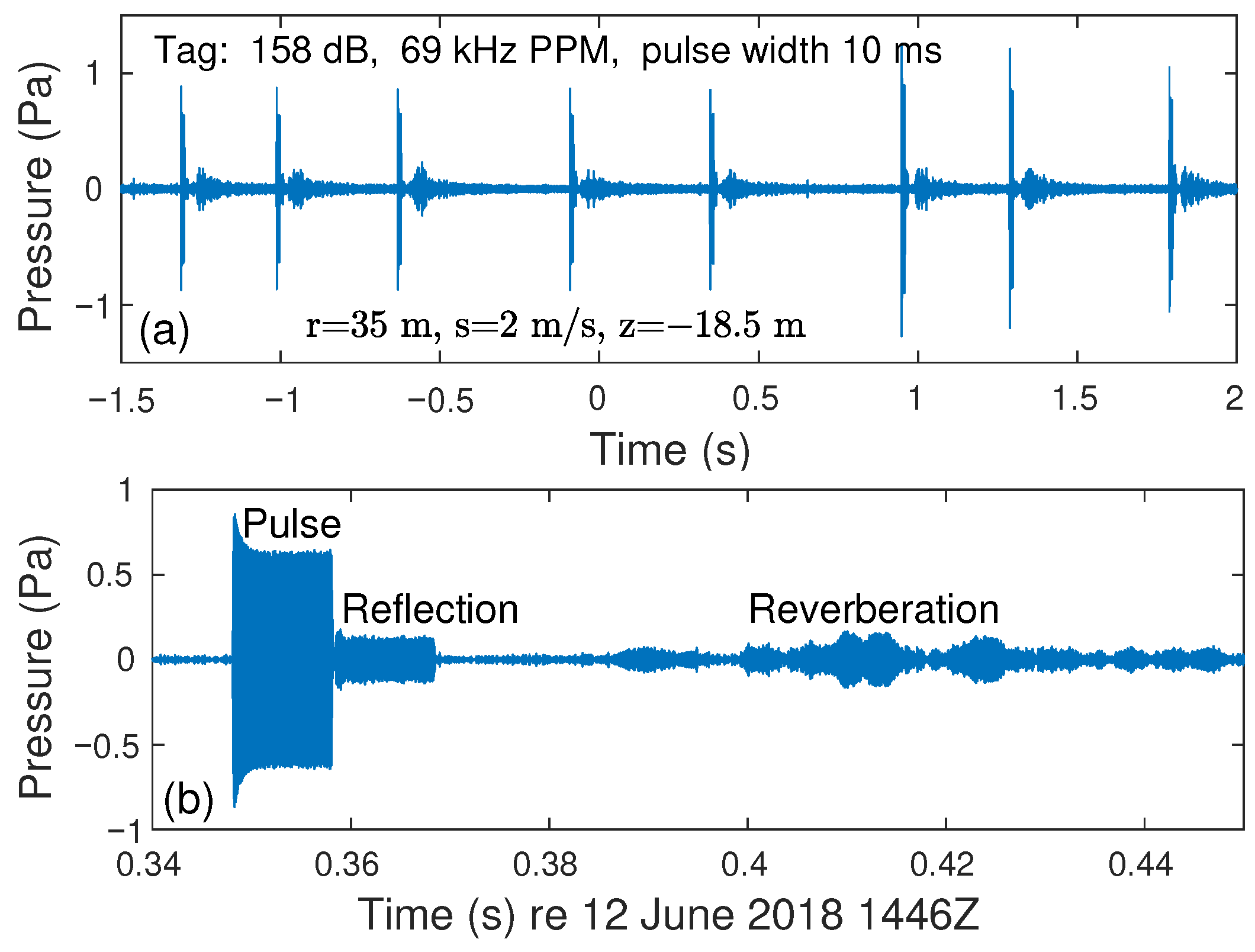Furthermore, at small range, close proximity detection interference (CPDI) [11] causes further uncertainty for signal detection [12]. A 69 kHz PPM tag signal encodes information according to the gaps between eight 10 ms pulses that are spaced over a few seconds (Figure A1a), so signals are transmitted infrequently because of the energy cost and the need to avoid interference by pulses originating from another tag. Few 69 kHz PPM signals can be transmitted before fast currents sweep a tagged fish beyond the detection range of a VR2W receiver, so few tagged fish are detected. This presents an impediment for estimating fish–turbine encounter probability because it is the encounters at high current speeds that are of the most interest.

Given the lower ambient sound level at higher frequencies [12], some of the tagging effort has shifted to using Innovasea 170 kHz high-residency (HR) tags in recent years. HR tags can transmit both 180 kHz PPM signals (eight pulses that each have 5 ms duration) and 170 kHz HR signals. HR signals encode information by abrupt phase changes within a 6 ms pulse (Figure A2), so HR signals can be transmitted much more frequently than PPM signals and many signals can reach a moored HR2 receiver before the current sweeps a tagged fish out of range. Alewives carrying HR tags that transmitted signals every 1–2 s were detected making many passes through the Minas Passage on flood and ebb tides [3], even though the HR2 receiver array monitored only a small portion of the width of the passage. The apparent advantages of HR tags motivates the present measurements of their detection efficiency as a function of range and current speed.

HR technology has additional capabilities that were judged to be of potential use at our study site. The ability of HR2 receivers to separately identify a HR signal and its reflection allows the calculation of range between a receiver and a transmitting tag that is at a known depth. HR signals reflected from the sea surface can also be used to monitor the depth of a HR2 receiver. These capabilities turned out to be crucial for measuring detection efficiency, and the ability of the HR2 receiver to detect both 170 kHz HR and 180 kHz PPM signals enables a clear comparison of detection efficiency for those two signal types.

2. Materials and Methods

2.1. Moorings Design and Instrument Layout

Seven moorings were deployed for 32 d (9 April to 11 May 2021) on the volcanic plateau within the TED area (Figure 1). The line of moorings was orthogonal to the flood–tide current velocity. Each mooring consisted of a 240 kg anchor (a steel chain link) that was tethered by a 3 m riser chain to an acoustic release that was housed within the streamlined hull of a SUBS-Model A2 (Open Seas Instrumentation Inc., Musquodoboit Harbour, NS, Canada). Ideally, the moorings would hold HR2 receivers well clear of the seafloor to prevent the blocking of transmission paths but strong, turbulent currents make severe mooring tilt inevitable using the available buoyancy-based, mooring technology [12]. The location was selected for its relatively flat and regular seafloor, which was anticipated to minimize the blocking of sound signals traveling between moored HR2 receivers.

Mooring deployment was during low tide with the intent of separating moorings by 50 m. Currents are never really slack in the TED area, so navigation is difficult.

Table 1. Mooring locations and depths at low tide.

Site	Latitude	Longitude	Depth (m)	Device	HR TX-Interval (s)
1	45.3623	−64.4316	34	Tag	1.8–2.2
2	45.3628	−64.4314	33	HR2	4–6
3	45.3634	−64.4310	32	HR2	25–35
4	45.3640	−64.4308	34	HR2	4–6
5	45.3644	−64.4304	34	HR2	4–6
6	45.3650	−64.4300	34	HR2	4–6
7	45.3656	−64.4296	33	Tag	1.8–2.2

documents the research vessel position at the time each mooring was released overboard from the stern. The research vessel’s GPS was about 10 m forward of the drop position, so acoustic methods must be used to check and refine estimates of the mooring separation. HR tags were attached to the top of the SUBS tail fin at sites 1 and 7. HR tags transmitted 143 dB signals with 170 kHz HR signals set to a random delay interval of 1.8–2.2 s and 180 kHz PPM signals set to 15–25 s delay. Due to a miscommunication with the manufacturer, both of the HR tags turned off at about 1832 UTC on 23 Apr 2021, a little short of halfway through the experiment. It was intended that all HR2 receivers be set to transmit 143 dB HR signals within a random delay interval of 4–6 s, but the delay interval was mistakenly set to 25–35 s for site 3.

Every 10 min, the HR2 receivers recorded water temperature and the tilt angle of the HR2 from vertical. When using water temperature to estimate sound speed, 10 min sampling is adequate but underresolves fluctuations in SUBS orientation. Nevertheless, in a statistical sense, the tilt measurements indicate whether or not a SUBS maintains a streamlined orientation relative to the current.

2.2. Types of HR Signals That Are Detected by a HR2 Receiver

A HR2 receiver records detected signals according to the time they are detected and their identity. Presently, we define five types of HR signals that are detected by HR2 receivers. For a given purpose, detected signals may be useful or a hindrance, depending upon their type.

Type HR${}_{1\mathrm{d}}$ are signals that travel along a direct path from some other source to the detecting HR2 receiver. The other source might be a tag or a different HR2. Type HR${}_{1\mathrm{r}}$ are signals that are transmitted from some other source but are reflected off the sea surface before reaching the detecting HR2.

Type HR${}_{\mathrm{SELF}}$ is classified by Innovasea as a “SELF DET” and is a HR signal that a HR2 both transmits and records at the time of transmission. Type HR${}_{\mathrm{SELFr}}$ is when a HR2 receiver detects a reflection of its own HR${}_{\mathrm{SELF}}$ transmission. HR${}_{\mathrm{SELFr}}$ signals are usually reflected from the sea surface but sometimes they are reflected from deeper objects nearby the mooring.

Rarely, the HR${}_{\mathrm{SELF}}$ transmission can interact with a very nearby object in such a way as to create a signal with a fake identity. Remarkably, the transmitting HR2 will correctly record the identity and time at which the HR${}_{\mathrm{SELF}}$ was transmitted and fractionally later will also record the time of arrival of the fake signal along with its fake identity. This will be called a HR${}_{\mathrm{FAKE}}$ signal. Very infrequently, the transmitting HR2 will detect such fake signals after they have been reflected from the sea surface. Sometimes, the fake signal is detected by an HR2 that is different from that from which it originated.

2.3. Removal of Some HR_1r for Estimating Detection Efficiency

Acoustic impedance is much greater in water than air, so the sea surface reflects sound very well [25]. A HR signal that is detected by a HR2 receiver (but was not transmitted by that receiver) might have traveled a direct path from the transmitter to the receiver, or it might have traveled a path corresponding to reflection from the sea surface. Sometimes, the same transmitted signal will be detected twice; first, the HR${}_{1\mathrm{d}}$ signal, and a fraction of a second later, the HR${}_{1\mathrm{r}}$. In such circumstances, the HR${}_{1\mathrm{r}}$ signals are easy to identify because the time lapse from the HR${}_{1\mathrm{d}}$ is very much less than the time lapse between successive transmissions (Table 1).

Let $N_{d\wedge r}$ be the number of transmissions that were detected after traveling both a direct (d) and (∧) reflected (r) path, corresponding to $2N_{d\wedge r}$ detected signals. For estimating detection efficiency, we must remove the $N_{d\wedge r}$ reflected signals that closely follow signals that traveled a direct path.

2.4. Removal of HR_1r for HR2 Synchronization and Separation

HR${}_{1\mathrm{r}}$ signals (received after reflection from the sea surface) are troublesome if included in the data set used for synchronizing clocks on two HR2 receivers and measuring the distance between those receivers. Usually, HR${}_{1\mathrm{r}}$ are also a hindrance when using an array of receivers to localize the position of a tagged fish, although they can also be valuable for such calculations providing special care is taken [26].

The total number of detected signals $N_{\mathrm{total}}$, from X transmissions, can be written in a form that is relevant for calculating mooring separation:

$$N_{\mathrm{total}}=N_{d\wedge \sim r}+N_{\sim d\wedge r}+2N_{d\wedge r}$$

(1)

where $N_{d\wedge \sim r}$ is the number of transmissions that were detected after traveling a direct (d) path and (∧) were not (∼) detected after traveling a reflected (r) path. $N_{\sim d\wedge r}$ is the number of transmissions that were not detected after traveling a direct path but were detected after traveling a reflected path. $N_{d\wedge r}$ transmissions were detected for both direct and reflected paths. As before, it is easy to remove the $N_{d\wedge r}$ reflections that immediately follow the detection of a direct-path signal, so the the number of detected transmissions is

$$X_{\det }=N_{d\wedge \sim r}+N_{\sim d\wedge r}+N_{d\wedge r}.$$

(2)

The number of undetected transmissions can be written $X_{\sim \det }=N_{\sim d\wedge \sim r}$, so the total number of transmissions is

$$X=X_{\det }+X_{\sim \det }.$$

(3)

That leaves $N_{\sim d\wedge r}$ troublesome reflected signals within the detected signals $X_{\det }$, which cannot be identified and removed before synchronizing clocks and calculating mooring separation. Let us, therefore, evaluate the extent to which those $N_{\sim d\wedge r}$ reflected signals are present.

HR2 synchonization and separation first requires matching a short sequence of transmissions to a sequence of detections. Such matching is best achieved when the proportion of transmissions that are detected following a direct path, $\beta$, approaches 1 from below, i.e., $\beta \to 1^{-}$.

Signals traveling both reflected and direct paths suffer signal attenuation and distortion as they travel through the turbulent water volume and both must rise above the same ambient noise level to be detected. These things affect the probability of detecting a transmission in a way that is similar for both direct and reflected paths and they scale as $\beta$. Reflected signals suffer additional distortion and scattering from a roughened sea surface, which introduces a probability $P_s$ that an incident signal will be reflected sufficiently cleanly for the possibility of detection. This suggests that $N_{d\wedge \sim r}$ scales as $\beta (1-P_s)$, $N_{d\wedge r}$ scales as $\beta P_s$, $N_{\sim d\wedge \sim r}$ scales as $(1-\beta )(1-P_s)$, and $N_{\sim d\wedge r}$ scales as $(1-\beta )P_s$.

When $P_s$ and $1-\beta$ are similarly small,

$$N_{d\wedge \sim r}\gg N_{d\wedge r}\approx N_{\sim d\wedge \sim r}\gg N_{\sim d\wedge r}$$

(4)

and the troublesome reflections are rare. More generally, the physical scaling above gives

$$\frac{N_{d\wedge r}}{N_{d\wedge \sim r}}\approx \frac{N_{\sim d\wedge r}}{N_{\sim d\wedge \sim r}}\approx \frac{P_s}{1-P_s}.$$

(5)

Using (2) to substitute $X_{\det }-N_{\sim d\wedge r}-N_{d\wedge r}$ for $N_{d\wedge \sim r}$ and remembering that $N_{\sim d\wedge \sim r}=X_{\sim \det }$, we see that (5) cross multiplies to give the following quadratic equation:

$$N_{\sim d\wedge r}^2+\left(N_{d\wedge r}-X_{\det }\right)N_{\sim d\wedge r}+N_{d\wedge r}{X}_{\sim \det }\approx 0$$

(6)

which can be solved for $N_{\sim d\wedge r}$. $N_{\sim d\wedge r}$ can then be substituted into (2) to evaluate $N_{d\wedge \sim r}$.

2.5. HR2 Depth Relative to the Sea Surface

When a HR2 receiver detects a reflection HR${}_{\mathrm{SELFr}}$ of its own transmission HR${}_{\mathrm{SELF}}$, then there is a high probability that that reflection was from the sea surface. In such circumstances, the vertical distance is the speed of sound c multiplied by half the time lapse between when the HR signal was transmitted and when it was detected. The speed of sound was calculated following [27] by using the temperature measured by the HR2, using hydrostatic pressure at half the mooring depth in Table 1, and by assuming $31.5$ ppt salinity. Previous measurements in the Minas Passage indicated salinities in the range of 30.5 to 32 ppt [28,29,30] with tidal excursion causing salinity to sometimes vary by as much as 1 ppt [29]. Current also influences sound wave propagation, but signal paths are approximately orthogonal to the current, so the effect is minimal.

Reflections from the sea surface give a gappy time series for the height of the water column above the HR2. For each day, at each site, a regression fit to tidal harmonics (M2, S2, N2, and M4) was then used to obtain a daily averaged estimate of depth along with its 95% confidence interval.

2.6. HR2 Synchronization and Site Separation

By taking care to reference the HR2 to UTC soon before/after mooring deployment/recovery, much of the clock skew could be removed. It is then less computationally difficult to pattern match a time sequence of HR${}_{\mathrm{SELF}}$ transmissions from one HR2 to a corresponding (possibly gappy) time sequence of HR${}_{1d}$ signals detected by a neighboring HR2. Times at which signals are detected and transmitted enable more accurate synchronization and calculation of the separation between receivers.

Consider that HR2 receivers ${\Re }_1$ and ${\Re }_2$ are separated by some unknown range r and that there is an unknown clock offset so that at an instant when receiver ${\Re }_1$ records time $t_1$, the receiver ${\Re }_2$ records time $t_2=t_1+t_{\mathrm{offset}}$. In order to calculate separation range r and the time offset, we write the travel-time equations for two signals. Receiver ${\Re }_1$ transmits signal i at time $t_{1Xi}$ and ${\Re }_2$ receives signal i at time

$$t_{2Ri}=t_{1Xi}+\frac{r}{c}+t_{\mathrm{offset}}$$

(7)

where c is the speed of sound. Receiver ${\Re }_2$ transmits signal j at time $t_{2Xj}$ and ${\Re }_1$ receives that signal at time

$$t_{1Rj}=t_{2Xj}+\frac{r}{c}-t_{\mathrm{offset}}$$

(8)

It is now trivial to solve the above equations for r

$$r=\frac{c}{2}\left(t_{2Ri}-t_{1Xi}+t_{1Rj}-t_{2Xj}\right)$$

(9)

and $t_{\mathrm{offset}}$

$$t_{\mathrm{offset}}=\frac{1}{2}\left(t_{2Ri}-t_{1Xi}-t_{1Rj}+t_{2Xj}\right)$$

(10)

as functions of the transmission and reception times that the two receivers recorded for signals i and j. The current has minimal influence on the calculation of r because moorings are aligned across the current (Figure 1).

2.7. Separation between Tags and HR2 Receivers

A first estimate of separations between moorings can be obtained from latitudes and longitudes in Table 1. Separations between HR tags and HR2 receivers were also calculated from the time lag ${\tau }_{\mathrm{lag}}$ between the reception of a tag transmission traveling a direct path and a path that reflected from the sea surface. In order to make this calculation, we assume that the HR2 receiver and the tag are at the same depth D below the seasurface. This amounts to synchronous signals being sent from two sources separated by $2D$ in the vertical. For sufficiently large D, this amounts to a large aperture. Using the Pythagorean identity, separation range r is then calculated as

$$r=\frac{4D^2-c^2{\tau }_{\mathrm{lag}}^2}{2c{\tau }_{\mathrm{lag}}}.$$

(11)

This equation is a simplification of a calculation [26] for obtaining the range and depth of a harbor porpoise (Phocoena phocoena). Lag distance $c{\tau }_{\mathrm{lag}}$ also varies with tidal elevation. Before applying (11), linear regression was used to remove tidal constituents (M2, S2, N2, M4) from $c{\tau }_{\mathrm{lag}}$.

2.8. Tidal Current and Significant Wave Height

The present study measures how the detection efficiency varies as a function of vertically averaged tidal currents computed from the finite volume coastal ocean model, FVCOM [16,17,31]. For present purposes, tidal currents and surface elevation were computed and stored at 10 min intervals at site latitudes and longitudes documented in Table 1. Modeled currents do not capture fluctuations associated with turbulent eddies but are otherwise representative of ADCP current measurements in the TED area [32].

Throughout this study, we will use s to denote the signed tidal current speed, so s is positive on the flood tide and negative on the ebb tide. Tidal elevation ℓ and significant wave height were measured north of the TED area (−64.4040${}^{\circ }$, 45.3690${}^{\circ }$).

3. Results

Measuring detection efficiency is not trivial in the TED area. Moorings may move, so range r between moorings must be measured throughout the study. Proper account must be taken of signals taking direct and reflected paths. The interpretation of signals transmitted over near-seafloor paths requires an assessment of vertical level for each mooring.

3.1. Transmission between HR2 Receivers: Reflected Signals

Table 2. The number of HR signals transmitted X and detected $X_{\det }$ between sites.

Sites	X	${\mathit{X}}_{\mathbf{det}}$	Number Removed ${\mathit{N}}_{\mathit{d}\wedge \mathit{r}}$	Troublesome Number ${\mathit{N}}_{\sim \mathit{d}\wedge \mathit{r}}$	$\mathit{\beta }$	${\mathit{N}}_{\mathit{d}\wedge \mathit{r}}/{\mathit{X}}_{\mathbf{det}}$$\approx {\mathit{P}}_{\mathit{s}}$
$2\leftrightarrow 3$	621,816	537,521	27,686	4619	0.8644	0.0515
$3\leftrightarrow 4$	620,704	452,490	30,101	12,349	0.7290	0.0665
$4\leftrightarrow 5$	1,053,057	932,725	51,033	7021	0.8857	0.0547
$5\leftrightarrow 6$	1,055,051	567,080	34,185	33,396	0.5375	0.0603

documents the number X of HR transmissions from one site and the number $X_{\det }$ of those that were detected by a neighboring site. The total number $N_{\mathrm{total}}$ of detected HR signals was $X_{\det }+N_{d\wedge r}$ because there were $N_{d\wedge r}$ transmissions that were detected after traveling both a direct and reflected path. For calculating the range between sites, it is important that the $N_{d\wedge r}$ reflections are removed. $N_{d\wedge r}$ is typically 5–6% of the detected signals, so failure to remove reflections can cause the estimates of detection efficiency to exceed 1.

Detected transmissions $X_{\det }$ include $N_{\sim d\wedge r}$ reflections that cannot be identified and removed but are troublesome for clock synchronization and calculating distance between HR2 receivers. The number of troublesome reflections that remain in the time series $N_{\sim d\wedge r}$ was calculated using (6), and values in Table 2 are consistent with scaling relationships (4). $N_{\sim d\wedge r}$ is small compared to $N_{d\wedge r}$, except for transmissions between sites 5 and 6. Nevertheless, we expect that $\beta$ and $P_s$ might vary with environmental conditions, so there may be times when $N_{\sim d\wedge r}$ is a smaller/larger proportion of $X_{\det }$ than the averaged values in Table 2 might indicate.

The detection of reflections is expected to depend upon physical factors which vary with respect to time. It is not possible to construct a time series of reflected signals, but it is possible to construct a time series of signals that were detected on both direct and reflected paths at each site. Stratifying this time series with respect to tidal elevation shows that reflections are 2.57 times more commonly detected when tidal elevation is below its 25th percentile than when it is above its 75th percentile. Stratifying this time series with respect to significant wave height shows that reflections are 5.15 times more commonly detected when the significant wave height is below its 25th percentile than when it is above its 75th percentile.

3.2. Vertical Coordinate of the HR2 Receivers

Mooring locations and depths (Table 1) could only be roughly determined at the time of deployment. Times at which an HR2 receiver transmits a self signal HR${}_{\mathrm{SELF}}$ and then detects the reflection of that signal HR${}_{\mathrm{SELFr}}$ can be used to determine the subsurface depth of the HR2 receiver. The subsurface depth of the HR2 receivers varies mostly due to the rise and fall of the tide (Figure 2), but at site 2, there is also a step-like depth increase for the latter half of the deployment. At site 4, some signals are reflected from a subsurface object (e.g., a boulder on the seafloor) that is initially about 10 m from the mooring, transitioning to about 12 m from the mooring and then disappearing during the latter part of the deployment. The inset in Figure 2 shows that reflections from the nearby object occur on the flood tide. This indicates horizontal mooring movement and forebodes that bathymetric features can interfere with signal reception.

Reflections of self signals from the sea surface give gappy time series of the subsurface depth. Reflections that were obviously not from the sea surface were first removed. At each site, a regression fit to tidal harmonics (M2, S2, N2, and M4) was then applied for each day of measurements, so the fitted mean gives daily-averaged subsurface depths (Figure 3). In the latter portion of the deployment period, the mooring at site 2 slipped downwards, whereas the mooring at site 6 dragged slightly upwards. Initially, all HR2 receivers were <0.7 m from the same level, but their levels varied by almost 2 m at the end of the experiment.

3.3. Separation of HR2 Receivers

Begin by eliminating the $N_{d\wedge r}$ HR${}_{1\mathrm{r}}$ signals. Pattern matching time sequences of transmissions to detections then gives values $\left(t_{2Ri},t_{1Xi},t_{1Rj},t_{2Xj}\right)$ for travel-time Equations (7) and (8). A pair of HR2 receivers can then be synchronized and their separation distance calculated using (9) and (10). An ensemble of many signals can be transmitted and received within a period that is sufficiently short for clock drift and site separation to have negligible change. Within an ensemble, there are relatively few outliers, and they are usually easy to recognize and remove. (Failing to remove the $N_{d\wedge r}$ signals results in many more outliers and makes their removal difficult and tedious.) Averaging each ensemble gave separation ranges.

Figure 4 shows that for the first few days following deployment, there is some small variation in the separation of sites 2,3 and of sites 4,5, but this is of little consequence for measuring detection efficiency. Left insets of Figure 4 show order 1 m changes in separation that are associated with tidal current as though some mooring anchors were dragged slightly back and forth with the tide. These small changes of separation are too large to be attributed to changes in the speed of sound that might be caused by tidal changes in hydrostatic pressure, errors in temperature measurements, or any physically plausible change in salinity.

Major variations in station separation (Figure 4) happened 26–28 April during spring tides (Figure 2) and were timed with the flood tide. This is consistent with the TED area having faster flood currents than ebb currents [16], so overall mooring displacement is most likely towards the east.

Separation between sites 2 and 5 changed little except for briefly moving a little closer together within the period 25 April to 2 May. In that same period, the right inset (Figure 4) shows that transmissions from the HR2 at site 5 are reflected from a nearby object for a time interval that is coincident with sites 2 and 5 being a little closer together. Figure 3 indicates the site 2 mooring settling into deeper water. The most straightforward interpretation is that the movement of site 5 accounts for most of the small change in separation between sites 2 and 5, whereas site 2 shuffled into a local hollow but otherwise was approximately stationary.

Given that site 5 moved little, site 6 moved by more than 100 m during 26–28 April 2021. Most likely, sites 3, 4, and 6 all moved to an extent that was consequential for measuring detection range. Nevertheless, the separation ranges shown in Figure 4 are sufficient for estimating the detection efficiency of signals transmitted by one HR2 and received by another, although different ranges apply at different times for the same pair of instruments.

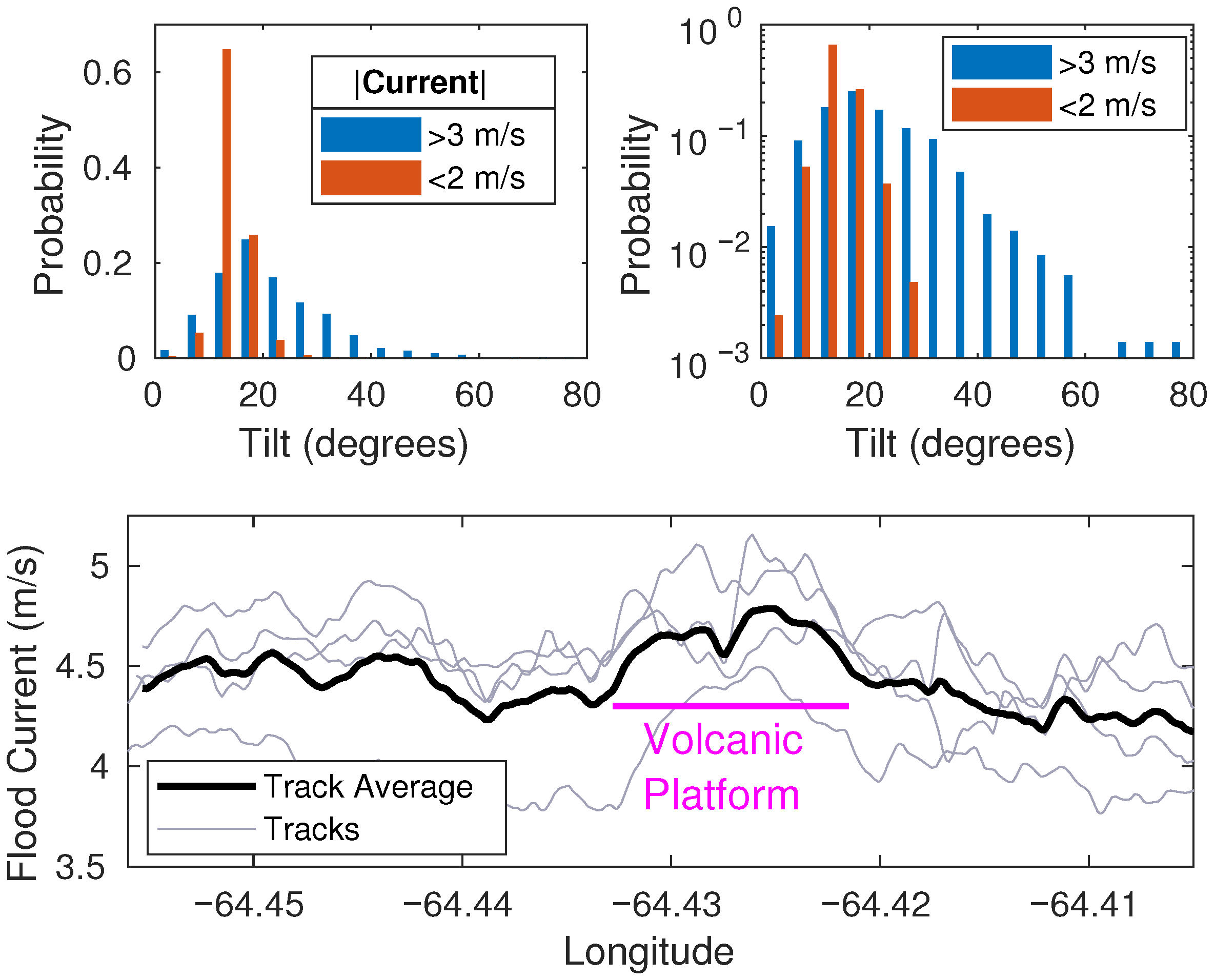
The 240 kg anchor weight was thought sufficient to prevent mooring movement on the volcanic plateau. Movement was greatest at site 6. Figure 5 shows HR2 measurements of the angle that the HR2 at site 6 was tilted from the vertical, which corresponds to SUBS tilt from a streamlined orientation into the current. Such tilt measurements cannot resolve pitch from roll and yaw, but they are indicative of lift and drag forces. When the current speed is less than 2 ms${}^{-1}$, the tilt is mostly in the range 10–15${}^{\circ }$ (red bars in Figure 5), which is consistent with a stable lift-generating SUBS alignment. These low speed tilts occur on both the flood (45%) and ebb (55%) tides. Current speeds greater than 3 ms${}^{-1}$ mostly happen (99%) on the flood tide. During fast flood tides, the tilt is distributed over a broad range, consistent with the unstable alignment of the SUBS. In order to visualize the full variation of tilt, the distributions are also plotted on a log-linear scale in Figure 5. Large changes in tilt suggest large forces. The forces that the SUBS applies to the anchor are not just drag and lift; the fluctuating SUBS movement also causes inertial forces due to the mass of the SUBS plus the virtual mass associated with the mass of the seawater that the SUBS displaces [33].

On the flood tide, drifters accelerate to achieve higher speed as they pass over the volcanic plateau of the TED area (Figure 5). On average, the speed increment approaches 0.5 ms${}^{-1}$ but individual drifter tracks show a good deal of variability that can be attributed to large-scale turbulent eddies. The flat, hard surface of the volcanic plateau may also make moorings vulnerable to movement. It is unclear whether mooring movement can be expected at sites that are not on the volcanic plateau.

3.4. Separation Ranges from Tags to HR2 Receivers

Ranges from tags (sites 1 and 7) to HR2 receivers were calculated from positions estimated at the time of deployment (second column of

Table 3. Ranges from tags to HR2 receivers. GPS ranges are from vessel position when the mooring was dropped overboard.

Sites: Tag,HR2	Drop Range (m)	${\mathit{\tau }}_{\mathbf{lag}}$ Range (m)
1,2	62	73
1,3	139	128
1,4	202	202
1,5	257	236
1,6	337	324
7,2	345	330
7,3	267	272
7,4	204	193
7,5	149	157
7,6	69	66

). Ranges from tags to HR2 receivers are only required up until 1832 23 April 2021 when the tags are turned off. During that time, there is little movement of the HR2 moorings at sites 2 through 5 (Figure 4). Temperature measurements were interpolated to the time of each signal to obtain sound speed c and therefore the lag-distance $c{\tau }_{\mathrm{lag}}$. After removing tidal constituents, $c{\tau }_{\mathrm{lag}}$ and subsurface depth $D=35.5$ m were substituted into (11) to obtain ranges in the third column of Table 3. The standard error in measurements of $c{\tau }_{\mathrm{lag}}$ causes <0.04% change in the calculation of range r except for the two greatest ranges in Table 3, where the change was ≈0.6%. On the other hand, varying D by $\pm 0.5$ m caused ≈3% change in range. Mooring separations obtained from ${\tau }_{\mathrm{lag}}$ are judged to be more reliable than those based upon estimates of the drop position.

3.5. Detection Efficiency: Tag to HR2

Separations between HR tags and HR2 receivers were stable while tags operated (Table 3). No record is kept of when each tag transmitted, but on average, each tag is expected to transmit 300 ± 1 times during a 10 min interval. For each 10 min time interval, there is a corresponding signed current speed s obtained from FVCOM. A specific tag–HR2 pair corresponds to a specific range, and detected transmissions are then distributed as a function of s in 0.25 ms${}^{-1}$ increments. The ratio of the number of signals detected to the number transmitted gives an estimate of detection efficiency $\rho \left(s\right)$ for HR signals between a tag–HR2 pair.

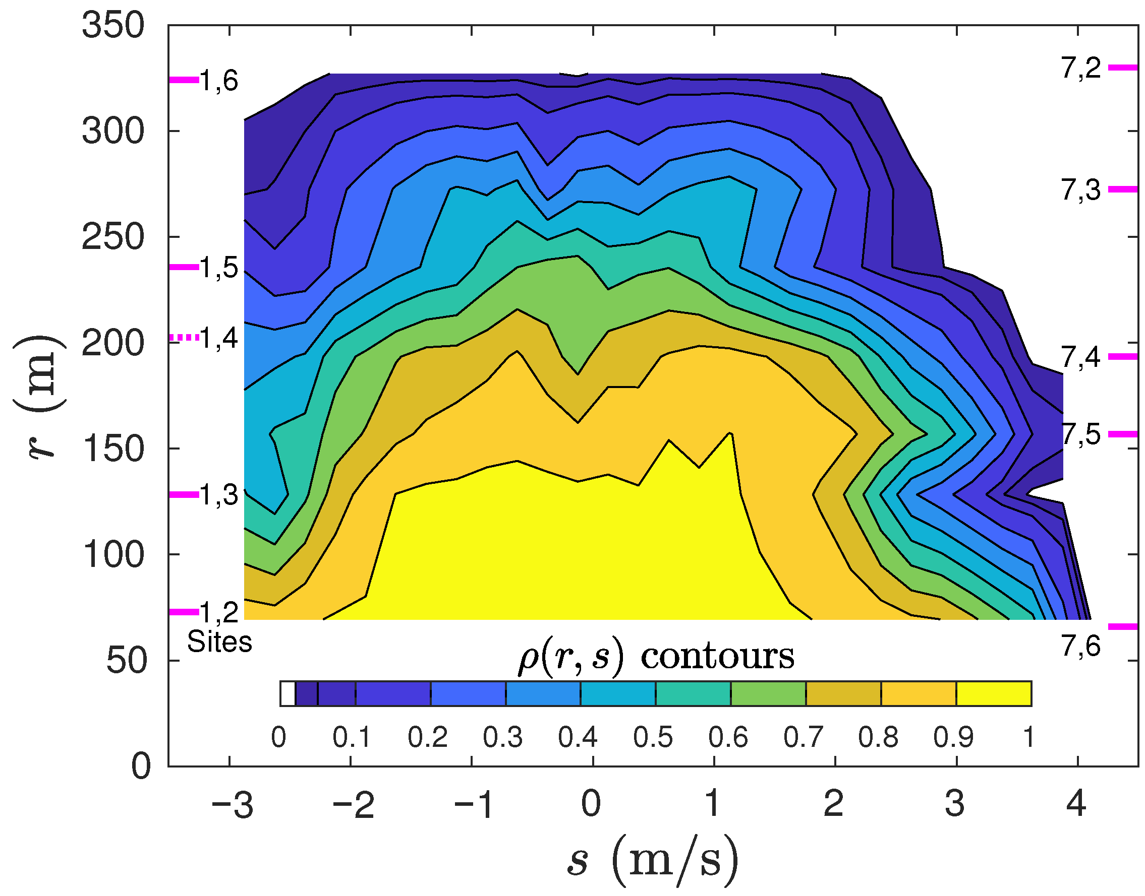
The receiver at site 4 detected the tag at site 1 poorly compared to the tag at site 7 (Figure 6), even though both transmission paths had very similar ranges. The poor reception of signals traveling the 1,4 path might result from the flood tide swinging the moorings so that the signal propagation path becomes blocked by a high spot in the bathymetry. High-resolution bathymetry is available for the study area but although ranges between sites are accurately determined, the positions of the moorings are not. It was not possible, therefore, to test whether or not a particularly high spot existed on or near the 1,4 path. Given that the ultimate goal of such receiver arrays is to detect tagged fish that are usually well clear of the bottom, it was deemed appropriate to neglect results from the 1,4 path.

With two tags each detected by five receivers, there are 10 transmitter–receiver pairs at ranges marked by magenta line ticks on the range axis of Figure 7. Ignoring the 1,4 path, Figure 7 shows contours of detection efficiency $\rho (r,s)$. It appears that the 1,5 and 1,3 paths might also have suffered some diminution of signal detection on the flood tide, less than that seen for the 1,4 path, but similar in form. Detection efficiency drops off rapidly when $\left|s\right|>2$ ms${}^{-1}$. Currents are faster on the flood tide, so estimates of detection efficiency are available for currents in the range $-3\le s\le 4$ ms${}^{-1}$.

3.6. Detection Efficiency: HR2 to HR2

HR2 moorings afford five receivers and five transmitters that transmit and receive HR signals throughout the study. The experiment was designed to measure two-way signal propagation along 10 transmission paths for a month. Figure 8 shows a time series of detection efficiency ${\rho }_{10}$ (calculated for 10-minute intervals) for HR signals transmitted between sites 4 and 5. Even for fast currents, ${\rho }_{10}>0.38$, while the range is ≈40 m. The mooring movement subsequently increases the range to >80 m, and similarly, fast currents cause a substantial reduction in ${\rho }_{10}$, although it always remains above 0. Results shown in Figure 8 contribute information near two ranges, and that is how they are used for the calculation of $\rho (r,s)$.

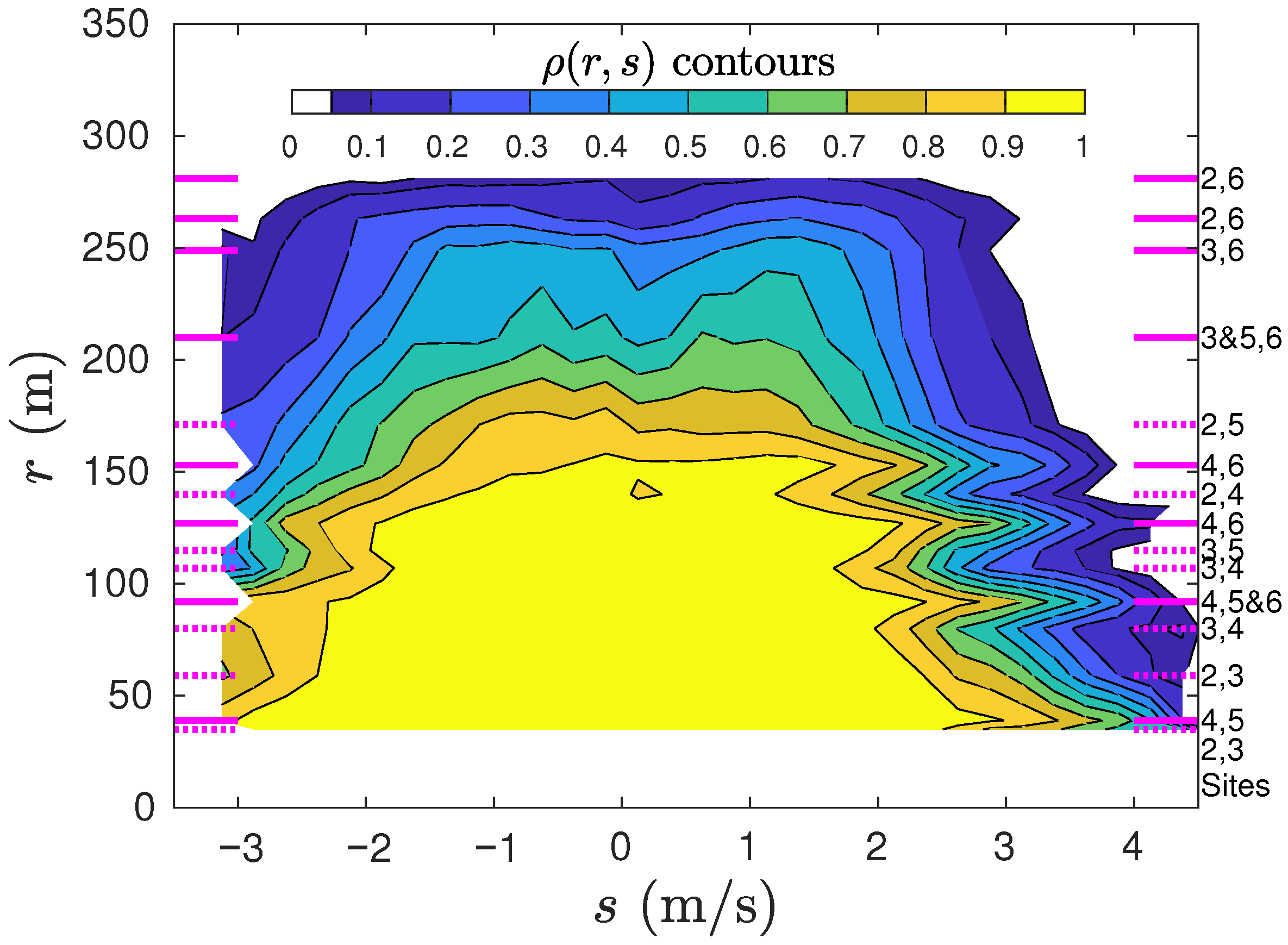
Figure 4 shows separation for four pairs of sites, one of which is largely stable while the others are quite variable. Considering the time series of separations between all HR2 sites, we identified 15 ranges that accommodated the majority of site-to-site separations to within a small uncertainty (

Table 4. Ranges used to calculate detection efficiency.

n	Separation (m)	Mooring Sites	Transmission Characteristic
1	$35\pm 2$	2,3	blocking
2	$39\pm 2$	4,5	no blocking
3	$59\pm 4$	2,3	blocking apparent
4	$80\pm 5$	3,4	blocking apparent
5	$92\pm 5$	4,5 & 5,6	no blocking
6	$107\pm 4$	3,5	blocking
7	$115\pm 4$	3,5	blocking
8	$127\pm 6$	4,5	no blocking
9	$140\pm 5$	2,4	blocking
10	$153\pm 5$	4,6	no blocking
11	$171\pm 5$	2,5	blocking
12	$210\pm 7$	3,6 & 5,6	no blocking
13	$249\pm 7$	3,6	no blocking
14	$263\pm 7$	2,6 & a few at 3,6	no blocking
14	$280\pm 7$	2,6	no blocking

). These ranges are marked with magenta on the vertical axis of Figure 9. Dotted magenta indicates ranges for which detection efficiency was poor compared with neighboring ranges. Poor detection efficiency may result from the signal path being blocked by bathymetry. Figure 3 shows that site 6 was the most elevated throughout the measurement period, and this corresponds to site 6 featuring in most ranges for which the detection efficiency was relatively high and the signal was deemed not to be blocked (Table 4).

It can be shown that poor performance at some ranges cannot be explained by statistical variability. Given the categorical nature of signal detection, the standard error of $\rho (r,s)$ is $\mathrm{s}.\mathrm{e}.\left(\rho \right)=\sqrt{\rho (1-\rho )/N}$, where N is the number of independent measurements used to calculate $\rho (r,s)$. Estimates of $\rho (r,s)$ are obtained from a great many instances and, except for the fastest flood/ebb currents, by averaging over many 10 min intervals. The standard error is too small to explain the variability of $\rho (r,s)$ that is seen in Figure 9. Rather, the variation in $\rho (r,s)$ is more likely associated with physical mechanisms (such as mooring tilt and bathymetric blocking) or errors made while modeling currents. Given this balance of probabilities, it seems that measurements in Figure 9 that are judged to suffer from blocking should be discarded when calculating values for $\rho (r,s)$ that are appropriate for detecting tagged fish that swim well clear of the seafloor.

Our experimental design did not adequately resolve how well signals are detected at ranges less than 40 m. Near the 40 m range, Figure 8 indicates that detection probabilities greater than 0.4 are achievable on the fast flood current during a spring tide. This raises the prospect that, to a reasonable approximation, results shown in Figure 7 and Figure 9 might be made complete if the detection efficiency can be estimated at a very small range.

3.7. Detection Efficiency at Very Small Range

The Innovasea HR2 receiver delivers very few (if any) false detections that correspond to a specified HR tag identity. For example, the tags (IDs 61676 and 61677) at sites 1 and 7 turned off 13.9 days into the present experiment. Before turning off, those tag IDs were detected a total of 2.6 million times by the five HR2 receivers but they were not detected during the subsequent 18.1 days of the experiment.

A different type of false signal was found. The HR2 receiver (serial number 461550) at site 3 transmitted a HR signal with ID 62554 every 25–35 s. That HR2 detected a HR${}_{\mathrm{FAKE}}$ signal with ID 25202 a total of 2444 times, and it was detected throughout the duration of the range test. (Innovasea confirmed that they had never manufactured a HR tag with that ID.) Analysis of times between consecutive HR${}_{\mathrm{FAKE}}$ transmissions corresponded to an underlying transmission interval in the range 25–35 s as though the time series was a gappy version of signals being transmitted by the HR2 at site 3.

Of the 2444 HR${}_{\mathrm{FAKE}}$ signals, 2433 were detected at site 3 with a lag of $(8.42\pm 0.12)\times {10}^{-4}$ s after the HR2 had transmitted its self-signal. That lag corresponds to a transmission distance of 1.250 m. Our physical interpretation is that the HR2 detected a reverberation of its self-signal that was caused by the two flotation spheres housed within the SUBS. The other 11 times that HR${}_{\mathrm{FAKE}}$ was detected at site 3, it lagged the self-signal by $0.0490\pm 0.0048$ s, which corresponded to detection after being reflected back from the sea surface.

For present purposes, regard the HR${}_{\mathrm{FAKE}}$ signal as having been transmitted 2444 times from site 3 and detected 2444 times at site 3. At greater range, HR${}_{\mathrm{FAKE}}$ was detected 503, 341, 267 and 27 times at sites 2, 4, 5 and 6, respectively. Blue bars in Figure 10 show the distribution of current when it is uniformly sampled though the experimental period. The current speed at the times when HR${}_{\mathrm{FAKE}}$ was detected at sites 2, 4, 5, and 6 had a different distribution (orange bars), which is consistent with the detection at long range being much less likely when the current speed is high. Current speeds at the times that HR${}_{\mathrm{FAKE}}$ was recorded at site 3 had a distribution (green bars) that was very similar to that for uniform sampling (blue). A fair interpretation is that, for current speeds in the TED area, very nearly all transmitted HR signals would be detected at the 1.25 m range.

3.8. Detection Efficiency and Detection-Positive Interval

The detection efficiency was modeled as a function $\rho (r,s)$. Temporal variation about this averaged formulation is expected because the ambient sound level influences signal detection, but ambient sound is only related to s in a statistically averaged sense. It is, therefore, important to assess how $\rho (r,s)$ might apply to the detection of the presence of a tagged fish during some interval $\Delta t$ that is sufficiently long so as to span many transmissions and sufficiently brief relative to tidal time scales so as to ensure that the same value of s applies.

Consider a tag that transmits every $\tau$ s that is present at a range r from an HR2 receiver when current is s. On average, the probability that a $\Delta t$ interval will be detection positive is

$$P_{\mathrm{pos}\Delta t}=1-{\left((1-\rho (r,s)\right)}^{\Delta t/\tau }.$$

(12)

$P_{\mathrm{pos}\Delta t}$ is thus obtained as 1 minus the probability that none of the $\Delta t/\tau$ transmissions are detected. The calculation depends upon an assumption that the detection of a transmitted signal does not influence the probability that the next transmission is detected.

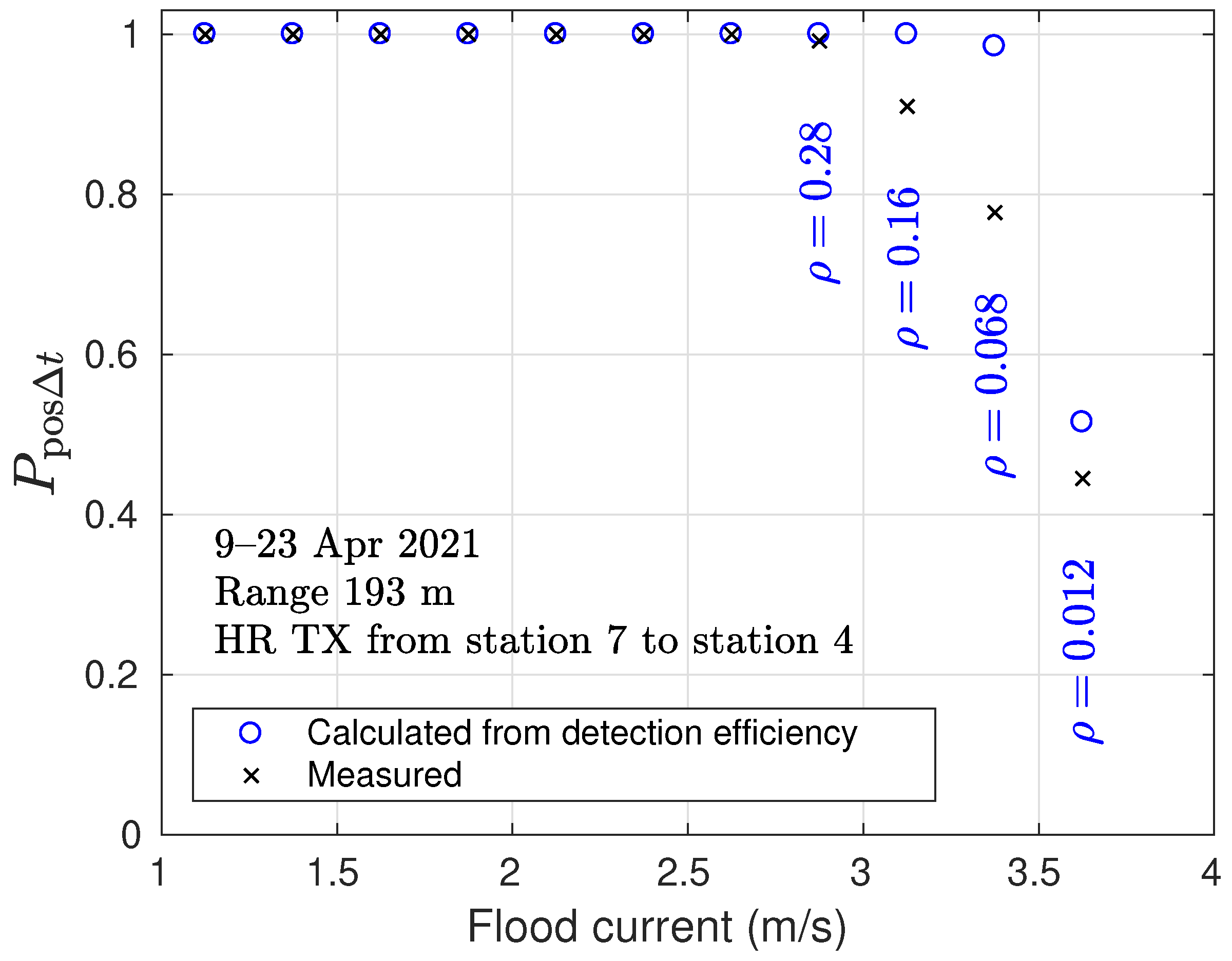
To test the applicability of (12), consider HR signals transmitted by the tag at site 7 and detected by the HR2 receiver at site 4 (Figure 6). The HR tag transmitted signals every $\tau =2$ s from a range of $r_{7,4}=193$ m for 13.86 days. Over that measurement period, each $\Delta t=120$ s interval was assessed to be detection positive if one or more signals were detected and otherwise detection negative. Black crosses in Figure 11 show the fraction of detection-positive intervals for each speed bin. Detection efficiency $\rho (r_{7,4},s)$ for HR signal propagation between these sites can be substituted into (12) to also estimate the fraction of detection-positive $\Delta t=120$ s intervals (blue circles).

At low current speeds, the detection efficiency is high and all intervals are detection positive, as expected. Lower detection efficiency at higher current speeds results in an appreciable fraction of the intervals being detection negative, and measurements show more detection-negative intervals than expected from (12). This demonstrates that the detection of a HR signal is not independent of whether the previous signal was detected. Obviously, if a given number of detected signals have a clumped distribution, then there will be more detection-negative intervals than for a random distribution.

3.9. Detection Efficiency and Area of Effective Detection

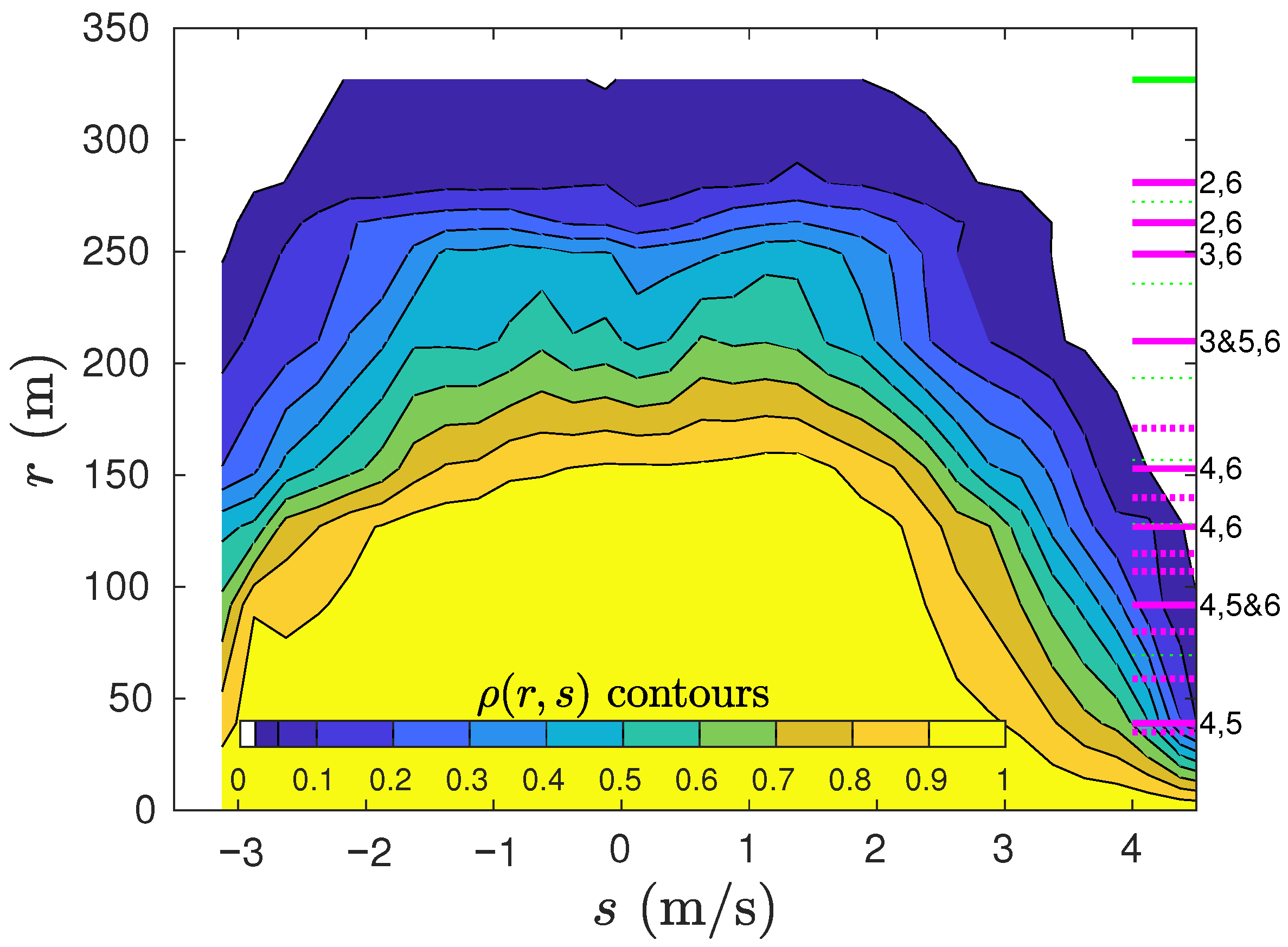
Our present interest is to use near-seafloor HR2 receivers to detect tagged fish that are sufficiently clear of the seafloor so that the signal path from fish to moored HR2 receiver is unlikely to be blocked by bathymetric features. Removing these blocked paths (Table 4), and extrapolating to all signals detected at near-zero range, gives the detection efficiency $\rho (r,s)$ as contoured in Figure 12.

If a tagged fish is detected by a HR2, then $\rho (r,s)$ provides a means to estimate the area within which the fish is expected to be located. Surrounding the position of the detecting HR2, an area of effective detection $A\left(s\right)$ can be calculated (13) by integrating over the horizontal plane:

$$A\left(s\right)=2\pi {\int }_0^{\infty }\rho (r,s)rdr$$

(13)

A is the area within which the tagged fish are effectively detected in a statistical sense. A might be conceptualized as an effective area within which the probability of detecting a tagged fish is 1 and outside of which the tagged fish would not be detected. Of course, no such sharp transitions exist, so sometimes a tagged fish within A will not be detected and sometimes a tagged fish outside A will be detected.

Given tag signals from $N_f$ tagged fish, where those signals are all detected throughout some time period T when the current is s, then an estimate of abundance $\mathcal{F}$ (number of tagged fish per unit area in the horizontal plane) can be obtained

$$\mathcal{F}=\frac{\tau N_f}{TA}$$

(14)

where $\tau$ is the tag transmission interval. This is the elemental concept that can be used to convert signals detected by a receiver to an estimate of fish abundance.

Corresponding to the idea of an effective area for detecting tags, the range of effective detection is defined by

$$\begin{array}{c}\hfill R\left(s\right)=\sqrt{\frac{A\left(s\right)}{\pi }}.\end{array}$$

(15)

If $\rho (r,s)$ is obtained from those transmission paths that do not appear to be blocked (Figure 12), then $R\left(s\right)$ is as plotted by the blue line in Figure 13. Including blocked transmission paths in $\rho (r,s)$ has the effect of diminishing R for fast flood currents (red line) but otherwise causes little change. Considering $\rho$ obtained from tag transmissions (Figure 9), and assuming that all signals are detected at a very close range gives a larger effective range in slow currents (yellow line in Figure 13) but underestimates the effective range in fast flood currents.

Having obtained the effective range, it is possible to describe the concept of the effective detection area $A\left(s\right)$ in a more quantitative way than above. Begin by calculating the inner area

$$A_{\mathrm{inner}}=2\pi {\int }_0^R\rho (r,s)rdr$$

(16)

by integrating only out to the effective radius R. The proportion of detected signals that originate within a physical space bounded by $r<R$ (within the effective area) is then given by the ratio $A_{\mathrm{inner}}/A$. For present measurements of detection efficiency, this ratio is about 0.8 when the current is slow. At higher current speeds, we might think of $\rho$ as being less step-like with respect to the range, which increases the likelihood that a detected fish may be outside the effective range.

3.10. Comparison of 170 kHz-HR and 180 kHz-PPM Signals

Tags at sites 1 and 7 transmit more frequently than the HR2 receivers and there was little mooring movement during the period for which tags transmitted. Thus, the detection of tag signals by the HR2 receivers provides the most reliable head-to-head comparison of detection efficiency for HR and PPM signals. Figure 7 shows the detection efficiency for tag HR signals, and the same procedure was used to obtain the detection efficiency for tag PPM signals. The ratio of detection efficiencies (Figure 14) shows that HR signals are better detected than PPM signals, particularly at large range and in fast currents.

4. Discussion

Using tidal MHK turbines [14,15] to harvest kinetic energy [16] may offset some carbon emissions caused by Earth’s large human population relying on fossil fuel [34]. To address concern about fish–turbine encounters, acoustically tagged fish were monitored in the Minas Passage since 2010. Most of that work used Innovasea 69 kHz PPM tags [2,4,6], but poor detection efficiency [12] hinders the reliable calculation of fish–turbine encounters when tidal currents are fast at the TED area in the Minas Passage [35].

The present results show that 170 kHz HR signals are better detected than 180 kHz PPM signals, and this is especially so as the range and current speeds increase. Additionally, the HR signals do not suffer from CPDI [11] and can be transmitted much more frequently than PPM signals. Considering all these factors, HR tags will be more effective than PPM tags for studying fish–turbine encounters in the Minas Passage. Recently, alewives with HR tags were measured making multiple passes through the Minas Passage TED area [3], so the presently obtained detection efficiency raises the prospect for the reliable calculation of the probability of alewife–turbine encounter.

Some illustrative progress on the MHK turbine encounter problem has been made using passive drifters [19]. While the collision probability of drifters with MHK turbines at the TED area is a matter of concern for engineers and scientists, it does not directly translate to the fish–turbine encounter probability because the drifters are usually deployed on quasi-stable tracks that pass through the Minas Passage, whereas fish might have quite different distributions depending on how they utilize their broader habitat [2,3,4,6]. Whereas a drifter track is well resolved in space and time, the position of an acoustically tagged fish is entirely unknown, except for those rare occasions when it is detected by a receiver. It is obvious when a tagged drifter passes by an array of receivers without being detected, but there is no way to know how many times a tagged fish passes by without being detected.

Detection efficiency measurements expand the utility of detected signals from tagged fish. Given accurate detection efficiency $\rho (r,s)$ and detected signals from tagged individuals belonging to a local population, Equation (14) provides an estimate for abundance, $\mathcal{F}$. If those signals were detected by HR2 receivers at the TED area in the Minas Passage, then $\mathcal{F}$ is an estimate of the number of tagged individuals per unit area. Fish in the water column are expected to approximately move with the water when the current speed is fast [19]. Given the vertical distributions of tagged fish [2,4], it is then straightforward to estimate the flux of tagged fish through a cross-current area that would, at some future time, be swept by the blades of a tidal MHK turbine. The probability that an individual belonging to a local population would encounter such a turbine can then be estimated by prorating according to the number of tagged individuals belonging to that population. Some fish might avoid the site when a MHK turbine is actually installed [36], while others may pass through a MHK turbine without being harmed [37], so the probability of encounter provides an upper limit on probability that an individual belonging to the population of interest may be harmed. Such metrics are directly relevant to population modeling [38], and thence to the objective regulation of MHK turbines and fisheries.

The ability of the HR2 receiver to identify and record HR signals in quick succession show that the probability was typically $P_d\approx 0.94$ that a received pulse followed a direct path as opposed to being reflected from the sea surface. The probability of detecting a PPM signal depends upon the reception of eight direct-path pulses without corruption by a reflected pulse. Making the physically plausible assumption that 69 kHz PPM pulses are reflected similarly to 170 kHz HR pulses, the probability of a PPM signal being corrupted by a reflected pulse is $1-P_d^8\approx 0.4$, which is consistent with CPDI [11,12] being caused by pulses reflected from the sea surface. This was not unexpected because seawater has much greater acoustic impedance than air [25], and non-breaking surface waves are characterized by broad troughs and crests with maximum steepness less than 1/7 [39]. Other high-frequency sound pulses were previously observed to reflect from the sea surface with relatively little distortion compared to the highly scattered signals that reflect off the seafloor [26]. Furthermore, the present work demonstrated that the probability of receiving a reflected signal decreases with increasing significant wave height, a result that mechanistically supports an observation by others of low CPDI for an experiment conducted in choppy waters [11].

Careful account must be taken of reflected HR signals in order to ensure that the same signal is not counted twice when measuring the detection efficiency. With respect to signals received from a tagged fish, there is no way to know whether an isolated signal traveled a direct or reflected path. Arguably, this does not matter for measuring detection efficiency because both instances represent a single detection for a single transmitted signal. While reflected signals may not warrant mention for acoustic localization in very shallow water [9], the present work demonstrates that they matter when the tag is at a greater depth because the source-to-receiver travel time of a reflected signal becomes quite different from that taking the direct path. Sometimes, that difference can be useful for localization [26], but it is usually a hindrance. The present work found that most reflected signals could be identified and removed because they closely followed a signal taking a direct path.

Provided that HR2 moorings are within range of one and other, it may be possible to calibrate $\rho$ for the times that tagged fish are detected. When tagged fish are detected, the concurrent measurement of $\rho$ might refine the estimate of the area of effective detection and thus abundance. Alternatively, when tagged fish are not detected, we can discern whether this might be due to a poorly performing HR2 receiver. A poorly performing HR2 receiver might also be indicated if it detects few reflections of its self signal compared to neighboring receivers. The separation of moorings can also be measured as a test that moorings have remained in place while fish are being monitored. Similarly, it is easy to monitor instrument depth when a HR2 receiver detects a reflection of its own HR${}_{\mathrm{SELF}}$ signal. Where bathymetry is highly variable—as it is south of the TED area—such depth monitoring might indicate a HR2 mooring has slipped into a crevasse. All these matters are of concern for the accurate interpretation of measurements made in the Minas Passage, where the available technology is pushed right to the edge of its capability.

Available mooring systems only enabled tags and receivers to be placed near the seafloor, whereas tagged fish that we study usually swim well clear of the seafloor when they are in the Minas Passage [2,4,40]. The range test could only measure signal paths that traveled from a near seafloor source to a near seafloor receiver. A 170 kHz sound wave has wavelength $\approx 8.7$ mm, and so, little energy can be expected to diffract around a much bigger object that obstructs the direct path from the transmitter to the receiver. Ray theory applies, and there is an acoustic shadow zone behind the object [41]. Such blocking is not representative for the detection of tagged fish that swim higher in the water column, so we presently consider it to be a source of error for the measurement of $\rho$. For that reason, measurements from some signal paths were discarded because comparison with other paths of similar length made it obvious that signals were blocked by obstacles on the seafloor (Table 4). This procedure can remove the most obvious errors, but it cannot ensure that those paths that remained do not, themselves, suffer from some degree of signal blocking, especially when fast currents tilt the mooring line [12]. Given that $\rho$ is of the most interest in fast currents, it is necessary to resolve the possibility of such systematic error in order to calculate probabilities of encounter with confidence.

To confirm that the present measurements of HR detection efficiency apply for a tagged fish, measurements can been made by suspending tags beneath a drifter that passes over a receiver array. It is logistically difficult to use drifting tags to measure $\rho$ for all current speeds and ranges, but quasi-stable trajectories [19] do pass through the Minas Passage when the current is fast and thereby provide a means to test the applicability of present measurements of $\rho$ under conditions of concern. Consider a tagged drifter (or tagged fish) that transmits with interval $\tau$ and moves at speed past a fixed HR2 mooring. The number of signals that are expected to be detected $E\left(N_{\det }\right)$ can be calculated by integrating $\rho$ over the path taken by the drifter and multiplying by the number of signals transmitted along the path. Whereas the path of a tagged fish is not known, GPS measurements can accurately give the path of a drifter that carries tags. If our estimates of $\rho$ are accurate, $E\left(N_{\det }\right)$ should be comparable with the number of detections that are observed $\mathrm{Obs}\left(N_{\det }\right)$ when the drifter passes by a receiver. Appropriate drifter measurements will be reported shortly [42].

5. Conclusions

• In fast tidal currents, it is most advantageous for an array of HR2 receivers to be spaced so that each HR2 can detect signals from its neighbors. This enables the time synchronization of receivers and mooring movement to be quantified. Additionally, it enables detection efficiency to be estimated concurrent with the time that a tagged fish is detected.
• Measurements of detection efficiency were variable over short intervals, and values were not independent from one interval to the next. Such correlation can influence the number of detection positive intervals. Further work is, therefore, necessary to verify that the present measurements of detection efficiency apply to the detection of tagged fish that quickly pass by receivers [42].
• Some of the present detection efficiency measurements were discarded because there were indications that bathymetry blocked the near seafloor signal paths. Further testing is required to confirm those indications and verify that the presently obtained detection efficiencies apply to signals from tags that are well clear of the seafloor [42].
• The concept of an effective detection area is introduced and can be calculated from detection efficiency. The effective detection area enables signals detected from tagged fish to be converted to an estimate of the abundance of tagged fish.
• Provided that drifter measurements [42] verify the utility of the present estimates of detection efficiency, there is every prospect of using detected signals from tagged fish to calculate fish–turbine encounter probability in the tidal energy demonstration area in the Minas Passage [43]. Encounter probability places an upper bound on the possibility of fish being harmed by MHK turbines and is, therefore, expected to be an important consideration for the regulation of MHK turbines under the Canadian Environmental Assessment Act, Fisheries Act, and Species at Risk Act.