Design and Analysis of a Decoupling Buoyancy Wave Energy Converter

Abstract

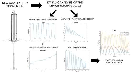
This study presents a new wave energy converter that operates in two phases. During the first phase, wave energy is stored, raising a mass up to a design height. During the second phase, the mass goes down. When going down, it compresses air that moves a turbine that drives an electrical generator. Because of this decoupling, generators that move much faster than seawater can be used. This allows using “off-the-shelf” electrical generators. The performance of the proposed design was evaluated via simulations. As the device operates in two phases, a different simulation model was built for each phase. The mass-rising simulation model assumes regular waves. The simulation results suggest that energy harvesting is near the theoretical maximum. Mass falling is braked by air compression. Simulations of this system showed oscillatory behavior. These oscillations are lightly damped by the drag against the walls and air. These oscillations translate into generated power. Therefore, smoothing is needed to avoid perturbing the grid. A possible solution, in the case of farms comprising dozens of these devices, is to delay the generation among individual devices. In this manner, the combined generation can be significantly smoothed.

1. Introduction

The United Nations has made one of its Sustainable Developments Goals (SDG) that, for 2030, “there will be affordable, reliable and clean universal energy access” [1]. Marine energies are among the clean energy resources available [2]. More specifically, wave energy is one of these sources that has been fully considered. In fact, 46 GW of wave generation is expected by 2050 [3]. Notwithstanding, these devices also have an environmental impact throughout their entire lives [4].

Wave energy resources are widely distributed. Particularly, the Atlantic Iberian nearshore is among the most promising European coastal environments for wave energy extraction [5]. However, wave energy has not yet been harvested as much as other renewables such as wind and solar [6]. Currently, research is focusing on power generation and operation [7] and on combining several sources, such as wind and wave in the same device [8].

Three operational principles were used for wave energy harvesting. These are the oscillating water column (OWC) [9], overtopping devices (OTD), and wave-activated bodies (WAB). The directional characteristics of wave energy converters (WEC) provide another classification. They can be point absorbers, terminators, or attenuators [10]. In addition, piezoelectric- [11] and triboelectric-based wave energy converters have been proposed. These types of energy converters are considered for powering sensor buoys. Other WECs have also been proposed to achieve this aim [12].

The performance of WECs has been analyzed numerically and is heavily dependent on their size. In fact, the annual absorbed energy per unit surface area was device-independent. The exception is a bottom-fixed oscillating flap which doubles the other devices analyzed [13].

The optimal buoy design should consider the sea conditions. Therefore, it can attenuate the ripple caused by short-period lippers and maximize the energy capture for long-period swells [14].

Several WECs were based on buoys. To enhance efficiency, they were tuned to resonate. However, most resonate at a single frequency. To widen their applicability, two-buoy WECs have three natural frequencies [15].

Two types of power take-off (PTO) systems have been proposed for buoys. Currently, the most commonly used system is based on a hydraulic transmission system and a conventional generator [16]. Another option is a direct drive linear generator [17]. In most cases, this linear generator has permanent magnets in its exciter [18].

Most of the WECs do not include energy storage. However, WECs generate energy through power surges. To smoothen this generation, energy storage is needed [19].

In this study, the design of a wave energy converter with decoupled buoyancy (WECDB) is presented. WECDB incorporates energy storage to decouple the wave motion and power generation [20]. The remainder of this paper is organized as follows: First, the WECDB design is explained in Section 2. Section 3 presents a dynamic analysis of this device. Section 4 presents a case study, followed by a discussion of the simulation results in Section 5. Finally, conclusions are presented in Section 6.

2. The Proposed WECDB Device

The components of the proposed WECDB, starting from the seabed, are shown in Figure 1. The device has a structure able to support the generating module elements. These are a base on the seabed (37) to which the WECDB is moored. From the mooring point (9), the link (10) ends in an inverted truncated cone surface. This surface guides waves to the float and is bonded to the WECDB base (11). A watertight chamber (5) is fixed on this base.

This chamber is cylindrical and is terminated by a conical cover. Inside the chamber, there is an inner pipe (2), also cylindrical. This inner pipe is mounted vertically on the lower base of the watertight chamber. Inside the inner pipe, there is an air turbine (4). The active mass (4) is mounted surrounding the inner pipe. This mass oscillates guided by the inner pipe and the watertight chamber walls. It has some anchoring points that bond it to the coupling–decoupling system.

The device includes a system for controlling its operation. This control system is composed of a computer (8) and its peripherals. These peripherals include position and speed sensors that should continuously measure the speed and position of both the float and the active mass. From this data, the computer will send commands to coordinate the performance of all the elements of the device.

A floating device (6) surrounds this enclosure. This float has a toroid shape and is connected to a coupling–decoupling system that connects it to the active mass. This system is composed of jaws (29) and cables (30).

Figure 2 shows the interior of the proposed WECDB. There is an active mass (3) inside the watertight chamber. This mass can move along an inner pipe (2). A turbine (4) is inside the inner pipe.

When the active mass descends, it behaves as a plunger on the air contained in the volume constrained by the inner pipe (2) walls, the watertight chamber (5) walls and base, and the lower surface of the active mass (3). The turbine (4), inside the inner pipe, is of axial flow and vertical shaft. It is located in the lower base of the watertight chamber. The turbine details are presented in Figure 3.

The WECDB has a coupling–decoupling system. This system, shown in Figure 4, is composed of several mechanical elements. The jaws (29) perform the coupling and decoupling of the float to the other module elements. When a wave rises, the jaws couple the float to a cable (30), decoupling it when a wave descends. At the active mass end, a ratchet (31) preserves the height of the active mass when a wave descends. In this way, the active mass accumulates with the rising of the wave’s height. The ratchet (31) liberates the descent of the active mass (3) once the design height is reached.

In addition, the coupling–decoupling system has brakes (41) joined to the ratchet. The brakes will stop the motion of the active mass when it approaches the lower base of the watertight chamber. The other mechanical elements of the system are the upper (40) and lower (39) pulleys of the cable (30), and several spools (32) where the cable is collected. The entire coupling–decoupling system is supported by a portal frame (38) fixed to the lower base of the watertight chamber.

The evolution of the device through a wave cycle starts from a valley. At this moment, the active mass rests over the base of the watertight chamber. As shown in Figure 5, when a wave starts rising, the control system couples, through a jaw (29), float, and cable (30).

With the float coupled to the cable, as a wave rises, the float thrust is transmitted through the cable to the active mass. Figure 6 shows the hydraulic thrust. When the thrust is larger than the active mass weight, the latter starts to rise.

When a wave descends, the float decouples from the cable, and the active mass is suspended in an elevated position through ratchets (31). The wave cycle repeats, and the active mass stores the potential energy up to the design height Hg. To generate energy, the active mass should descend from this height. The ratchets liberate the active mass, which descends under its own weight.

Simultaneously, the lower valves (48) are closed. Therefore, the active mass presses the fluid in the chamber between the active mass and the lower valves. At a certain pressure, the lower valves open and channel fluid flowing through the turbine. Figure 7 illustrates this process. The turbine moves the electric generator to generate electrical energy.

When the active mass reaches the base of the watertight chamber, the generation ends. Therefore, a new cycle can start when a new wave arrives at the WECDB.

The volume that surrounds the watertight chamber is in contact with the atmosphere, and thus it is always at atmospheric pressure. Notwithstanding, air moves in a closed circuit. After being turbined, the air exits through the upper part of the inner pipe (2). Then, it is recirculated inside the watertight chamber (5), crossing the upper valves (46). As the active mass rises, the lower valves (48) are open, so air can flow through them freely. In Figure 7 the symbols Δ and Δ’ refer to the plane of the valve. Δ’ shows its position in the main Figure 7 and Δ is a zenithal view of this plane. This airflow has low pressure and speed. It only occupies the volume freed by the rising of the active mass.

When dangerous conditions are detected (as during heavy storms), the computer stops the energy harvesting operation and puts the device in safe mode. In this mode, the active mass will be in its lowest possible position and the float will oscillate freely (decoupled from the cable).

3. Dynamic Analysis of the WECDB Device

In order to evaluate the performance of devices like the one previously described in Section 2, a model must be built. To this end, the equations that describe the physical response of the described device to some sea state must be determined. In order to obtain these equations, a dynamic analysis of the device is performed. This analysis is divided into two parts. The first one analyzes the active mass rise and the second analyzes the active mass descent.

3.1. Analysis of Active Mass Rising

As the horizontal movements of both the float and active mass were constrained, only vertical movements were considered (heave motion). To this end, a force analysis during the wave rising and descent was performed. Float movement is a consequence of the interaction of the buoyancy force F_BUOY, drag force, weight, cable tension T_CF, excitation force F_EX, and radiation force F_RAD.

The excitation force is caused by the incident waves on the float. The characteristics of these incident waves depend on the sea state that surrounds the device. Assuming regular (i.e., sinusoidal) waves, Equation (1) describes this force:

F_EX = f_e A cos (ωt + Φ)

(1)

where f_e, A, ω, and Φ are the force excitation coefficient, wave amplitude, wave frequency, and wave phase, respectively. The coefficient (f_e) was calculated using Equation (2):

$${\mathrm{f}}_{\mathrm{e}}=\sqrt{\frac{{8·\mathsf{\pi }·\mathsf{\rho }·{\mathrm{R}}_{\mathsf{\omega }}·\mathrm{g}}^3}{{\mathsf{\omega }}^3}}$$

(2)

where R_ω, ρ, and g are the radiation resistance, water density, and gravitational acceleration, respectively. The radiation force is given by Equation (3):

$${\mathrm{F}}_{{\mathrm{RAD}}_{ }}=-{\mathrm{m}}_{\mathsf{\omega }}\ddot{Z}-{\mathrm{R}}_{\mathsf{\omega }}\dot{Z}s$$

(3)

where m_ω, $\dot{Z}$, and$\ddot{ Z}$ denote the aggregated mass, float vertical speed, and acceleration, respectively. The aggregated mass and radiation resistance of a cylindrical body are [21]:

m_ω = 0.875·M

R_ω = ω·ρ·(2·π/3)·a³·ε·e^−2·k·l

(4)

where M, a, k, ε, and l denote the mass of the body, its radius, the angular wavenumber, a dimensionless coefficient, and half the cylinder height, respectively. The angular wave number is the inverse of the wavelength multiplied by 2·π. According to [21], ε is a function of the product of the angular wavenumber and the cylinder radius.

The buoyancy force depends on the float submerged volume (V_SUB) and the seawater density, as shown in Equation (5):

F_BUOY = ρ·g·V_SUB

(5)

The drag force depends on the seawater density and viscosity, float geometric characteristics, and relative speed between the float and water. Because of the usual values of these parameters, it is neglected in this analysis.

When a wave rises, the float is coupled to the tension cable. In addition, the submerged float volume changes. When the buoyancy force is greater than the other forces, the float rises. The buoyancy force depends on submerged float volume, as shown in Equation (6):

$$\mathsf{\Delta }{\mathrm{V}}_{\mathrm{SUB}}=\left\{\begin{array}{cc}0& \mathrm{i}\mathrm{f} {\mathrm{Z}}_{\mathrm{w}}-{\mathrm{Z}}_{\mathrm{F}\mathrm{L}}\le 0\\ {\mathrm{S}}_{\mathrm{fl}}·\left({\mathrm{Z}}_{\mathrm{w}} - {\mathrm{Z}}_{\mathrm{F}\mathrm{L}}\right)& \mathrm{i}\mathrm{f} 0<{\mathrm{Z}}_{\mathrm{w}}-{\mathrm{Z}}_{\mathrm{F}\mathrm{L}}\le {\mathrm{H}}_{\mathrm{fl}}\\ {\mathrm{V}}_{\mathrm{fl}}& \mathrm{i}\mathrm{f} {\mathrm{H}}_{\mathrm{fl}}\le {\mathrm{Z}}_{\mathrm{w}}-{\mathrm{Z}}_{\mathrm{F}\mathrm{L}}\end{array}\right.$$

(6)

where H_fl, Z_w, and Z_FL are the total float height, vertical displacement of the sea surface, and vertical displacement of the float. Figure 8 shows the displacements.

Equation (7) describes the float movement. This equation is Newton’s second law. This law states that the acceleration of a body is proportional to the summation of forces applied to it and inversely proportional to its own mass.

$$\begin{gathered} \mathrm{M}·\ddot{\mathrm{Z}}={\mathrm{F}}_{\mathrm{buoy}}+{\mathrm{F}}_{\mathrm{ex}}+{\mathrm{F}}_{\mathrm{rad}} -{\mathrm{T}}_{\mathrm{cf}} -{\mathrm{F}}_{\mathrm{grav}} \\ \mathrm{M}·\ddot{\mathrm{Z}}=\mathsf{\rho }·\mathrm{g}·∆{\mathrm{V}}_{\mathrm{sub}}+{\mathrm{f}}_{\mathrm{e}}·\mathrm{A}·\cos \left(\mathsf{\omega }·\mathrm{t}+\mathsf{\phi }\right)-{\mathrm{m}}_{\mathsf{\omega }}·\ddot{\mathrm{Z}} -{\mathrm{R}}_{\mathsf{\omega }}·\dot{\mathrm{Z}} -{\mathrm{T}}_{\mathrm{cf}} -{\mathrm{M}}_{\mathrm{fl}}·\mathrm{g} \end{gathered}$$

(7)

When a wave rises, the T_CF is equal to the weight of the active mass (M_ACT), but when a wave descends it is equal to zero. As previously explained, when a wave rises, the active mass is coupled to the float by the tension cable. As a consequence of this coupling, when a wave rises, the moving mass M is the mass of the float plus the mass of the active mass. However, when a wave descends, the active mass is decoupled from the float. Therefore, when a wave descends, the moving mass M is only the mass of the float.

3.2. Analysis of Active Mass Descent

After a sufficient number of wave cycles, the M_ACT reaches the design height. The gravitationally stored energy can then be transformed into electrical energy. To this end, the ratchets are liberated. Then, the M_ACT falls owing to gravitational force. As the mass moves inside a closed chamber, when the mass descends, the air pressure in the chamber increases. This increase in pressure, as well as the friction against the walls, reduces the M_ACT speed. The M_ACT movement is described by Equation (8), which, again, is Newton’s second law.

$$\begin{gathered} {\mathrm{M}}_{\mathrm{Act}}·\ddot{\mathrm{Z}}= \\ \frac{1}{2}·{\mathrm{c}}_{\mathrm{a}}·{\mathsf{\rho }}_{\mathrm{air}}·{\mathrm{S}}_{\mathrm{Ac}{\mathrm{t}}_{\mathrm{Mass}}}·\dot{\mathrm{Z}}·\left|\dot{\mathrm{Z}}\right|+\left({\mathrm{P}}_{\mathrm{int}} - {\mathrm{P}}_{\mathrm{ext}}\right)·{\mathrm{S}}_{\mathrm{Ac}{\mathrm{t}}_{\mathrm{Mass}}}-\left(1-\mathrm{sign}\left(\dot{\mathrm{Z}}\right)·\mathsf{\mu }\right)·{\mathrm{M}}_{\mathrm{Act}}·\mathrm{g} \end{gathered}$$

(8)

The first term of the second side of Equation (8) is the viscous drag force. The second term is the consequence of pressure variation inside the chamber when the active mass moves. Moreover, the third term represents the weight and the drag against the walls. This last drag has a sign that is always opposite of the active mass speed sign. Assuming adiabatic compression, the interior pressure can be expressed as Equation (9):

$${\mathrm{P}}_{\mathrm{int}}·{\mathrm{V}}_{\mathrm{int}}^{\mathsf{\kappa }}={\mathrm{P}}_0·{\mathrm{V}}_0^{\mathsf{\kappa }}={\mathrm{P}}_{\mathrm{int}}·{\left({\mathrm{S}}_{\mathrm{Ac}{\mathrm{t}}_{\mathrm{Mass}}}·\mathrm{Z}\right)}^{\mathsf{\kappa }}$$

(9)

where κ is the ratio of the specific heats. An additional consequence of this compression is a change in air temperature. This temperature change can be calculated assuming that the air is a perfect gas. Obviously, the air density varies according to all these changes. When the chamber is closed, the change in air density is inversely proportional to the change in interior volume.

To generate energy, compressed air should be allowed to flow through an air turbine. To this end, a valve is opened when sufficient pressure in the closed chamber is reached. Once the valve is opened, the airflow exits the closed chamber, modifying the air mass in the chamber. This modification of the air mass modifies both the interior air density and interior air pressure.

Assuming isentropic flow, air mass flow is calculated using Equation (10). According to this equation, the mass flow will vary, mainly due to changes in the interior pressure. The effect of interior temperature changes is lower on mass flow.

$$\dot{m}=\frac{P_{int}}{\sqrt{R·T_{int}}}·S_{turb}·\sqrt{\frac{2·\kappa }{\kappa -1}·{\left(\frac{P_{ext}}{P_{int}}\right)}^{\raisebox{1ex}{$2$}\!\left/ \!\raisebox{-1ex}{$\kappa $}\right.}·\left[1-{\left(\frac{P_{ext}}{P_{int}}\right)}^{\raisebox{1ex}{$\left(\kappa -1\right)$}\!\left/ \!\raisebox{-1ex}{$\kappa $}\right.}\right]}$$

(10)

4. Case Study

A device with the dimensions shown in Figure 9, Figure 10 and Figure 11 was considered. As the active mass rise is decoupled from its descent, two models were developed. The first model integrates Equation (7) taking into account Equation (6). The second model integrates Equation (8) taking into account Equations (9) and (10).

The dimensions of this device have been carefully chosen to maximize energy harvesting without violating the maximum point absorber restrictions, i.e., its diameter is sufficiently lower than the design wavelength. The float has an inner and outer radius of 6.3 m and 11.7 m, respectively. Its volume is 1590.16 m³. The active mass has a volume of 188 m³ and a mass of 776,000 kg.

The watertight chamber is inside the float. Its outer radius is 5.46 m. Concentric to the watertight chamber, the inner pipe has a radius of 1.11 m. The total height of the watertight chamber is 70 m, up to the vertex of the conical rooftop. Inside this chamber, under the active mass in its upper position, there are 4510 m³ of air.

Figure 12 shows the Simulink model that simulates active mass rising. This model sends to the workspace the variables whose evolution will be plotted.

Table 1. Main dimensions of the proposed device.

Symbol	Quantity	Value
A	Wave amplitude	3 m
T	Wave period	8 s
ρ	Seawater density	1026.7 kg/m3
g	Gravity acceleration	9.807 m/s2
ω	Angular frequency	0.7854 rad/s
a	Float outer radius	11.70 m
Sfl	Float cross-section	305.8 m2
Hfl	Float height	5.2 m
Mfl	Float mass	4.893 × 104 kg
MAct	Active mass	7.666 × 105 kg
ε	Coefficient	0.04 (dimensionless)

lists the values used in the model shown in Figure 12, Figure 13 and Figure 14 showing the evolution of the M_ACT height and water level, respectively.

As the system input is a regular wave, the system output is also regular. This means that every cycle is similar to the previous one. As Figure 13 shows, the device “rectifies” the oscillatory movement of the float. For this reason, the active mass rises steadily up to the design height.

Once stationary behavior has been reached, the M_ACT rises 3.3 m per cycle. This implies a stored energy of 24.8 MJ per cycle. Therefore, an average power of 3.1 MW is stored. The average incident power per unit width is [22]:

P_I = (1/2)·ρ·g·v_g·A² = 282.86 kW/m

(11)

where v_g denotes the group velocity. When the float diameter was 22.26 m and the wave period was 8 s, the incident energy was 50.4 MJ. The maximum extracted power for an axisymmetric device was [23]:

P_I/k = 4.5 MW

(12)

As it is well known, real sea states are not composed of regular waves. So, the performance of the designed device will be checked against more realistic waves. To this end, the well-known Pierson and Moskowitz spectrum will be used [24]:

$$S\left(\omega \right)=\frac{\alpha ·g^2}{{\omega }^5}·e^{-\left[\beta ·{\left(\frac{{\omega }_0}{\omega }\right)}^4\right]}$$

(13)

The total energy of the spectrum is proportional to the integral of the above spectrum for every value of ω:

$$A^2={\int }_0^{\infty }S\left(\omega \right)·d\omega =\frac{\alpha ·g^2}{4·\beta ·{\omega }_0^4}$$

(14)

The aforementioned reference [24] provides values for the parameters α = 8.1 × 10⁻³ and β = 0.74. In order to make a fair comparison with the regular wave case previously studied, ω₀ will be chosen in such a way that both waves have the same energy:

$${\omega }_0=\sqrt[4]{\frac{\alpha ·g^2}{4·\beta ·A^2}}=0.4135 \raisebox{1ex}{$rad$}\!\left/ \!\raisebox{-1ex}{$s$}\right.$$

In order to perform simulations, the spectrum defined by Equation (13) should be discretized [25]. Therefore, it can be simulated as a Fourier series instead of a single regular wave. Figure 15 shows the evolution of the active mass rising. As expected, the rising of the active mass is now irregular. Also, it takes more time for the mass to rise to the design height.

After the M_ACT reaches the design height (50 m in the case study), the gravitationally stored energy can be transformed into electrical energy. In this case, Equation (8) applies. To simulate the evolution of the system, another Simulink model was developed. This is illustrated in Figure 16. This model also sends to the workspace the variables whose evolution will be plotted.

The remaining parameters of the system are provided in

Table 2. Main dimensions of the power extraction device.

Symbol	Quantity	Value
ca	Viscous drag coefficient	0.4 (dimensionless)
SActMass	Surface of the active mass	77.98 m2
PExt	Atmospheric air pressure (at sea level)	101.325 kPa
µ	Sliding friction factor	0.04 (dimensionless)
κ	Ratio of specific heats (air)	1.4 (dimensionless)
R	Perfect gas constant	287.1 m2/(s2·K)
	Reference temperature at sea level	288.15 K
	Air density at reference conditions	1.225 kg/m3
Sturb	Cross-sectional area of the turbine	0.2619 m2

:

The simulation starts with the active mass suspended at the design height. Then, it is allowed to fall freely. The active mass falling is braked by drag and by the increase in interior pressure. Once an interior pressure larger than two times the exterior pressure is reached, the valve that allows compressed air to enter the turbine is open. Then, the air turbine accelerates, and an electric generator coupled to it starts generating electrical power.

Figure 17, Figure 18 and Figure 19 show the results of the simulations. As can be seen in Figure 17, the descent of the M_ACT is oscillatory, corresponding to a classic mass-spring system. In this case, the spring behavior corresponds to air compression in the chamber.

These oscillations are reproduced in the interior pressure, as shown in Figure 18. Consequently, the power available to the air turbine exhibits these oscillations. Figure 19 shows the evolution of air turbine power.

5. Discussion

A force analysis of the wave float interaction was performed. The previously described differential equations were integrated using the well-known and widely tested Dormand–Prince integration scheme. According to simulations, the raising of the M_ACT results in good performance. The hydrodynamic efficiency of this device for regular waves is 49.2% (24.8/50.4). This efficiency compares favorably with other heaving WEC systems [26]. Their hydrodynamic efficiencies (obtained by simulation) are mostly lower, varying between the 16% of a “single cylindrical body” and the 30% of the Danish Wave Energy Program System (30%). Only the Wavebob provides efficiencies similar to the device proposed here (between 40 and 51%) [27].

According to the results shown in Figure 13, an electrical generation cycle could be obtained after two minutes (120 s) of wave energy harvesting. As this generation cycle lasts one minute (approximately), a minimum of three devices are needed to obtain continuous power generation. However, this time is obviously dependent on the sea state. For example, when irregular waves were considered, this time was longer.

When the M_ACT was unlocked, its height oscillated, as shown in Figure 17. This was due to the spring effect caused by the compression of air in the watertight chamber. This oscillation is dampened by the air and wall drag, and the energy generation in the turbine. All of these components are very small. The wall drag is small due to the low sliding friction factor. The air drag is low due to the relatively low mass speed (maximum value near 15 m/s). Regarding energy generation, during its first cycle, the average power was (a little lower than) 4 MW and the average power of the descending mass during its first cycle was 48 MW. This explains why the damping of the oscillation is very low. This oscillation was also reproduced in the watertight chamber air pressure, as shown in Figure 18.

The available power in the air turbine depends on the air pressure in the watertight chamber. Therefore, it oscillated, as shown in Figure 19. This power fluctuation can be reduced by combining several devices in a wave farm. Thus, some smoothing is achieved due to the delay in the power generation start time between different devices. In order to explore this possibility, several simulations were performed using two and four devices. In the case of two devices, a delay between them of 3 s (half of the fluctuating power period) was assumed. In the other case (four devices) a delay among them of 1.5 s (one-fourth of the fluctuating power period) was considered. Figure 20 shows the resulting combined power.

In order to quantify the smoothing, the average and standard deviation power were calculated. For one device, the average power was 2.7 MW and the standard deviation was 2.33 MW. For two devices, the values were 4.9 MW and 2.33 MW, respectively. And for four devices, they were 12.4 MW and 2.33 MW, respectively. Therefore, average power increases with the number of devices but the standard deviation is constant. Consequently, the power fluctuation reduces when the number of devices increases. So, using a large enough number of devices, a smooth enough generated power is achievable.

Another way to reduce power fluctuations is proper rotor inertia [28]. However, this option will not be considered here. Notwithstanding, the purpose of this device is not to be the only, nor the main, generator of any grid. Its purpose is to contribute to energy generation in a grid. Every grid can absorb some power fluctuations, so, the proposed device should be connected to a large enough grid. This requirement may be a limiting factor on islands (especially small islands) but not in larger power systems.

6. Conclusions

The performance of a new wave energy converter was analyzed. This analysis assumed regular waves. The device operates in two phases. During the first phase, a mass is raised to a design height by seawater movement using a mechanical rectifier. Under the case study hypotheses, with a 3 m wave amplitude and 8 s wave period, the device needs two minutes to raise the active mass up to the design head of 50 m. During the second phase, the mass falls, compressing air. This air moves a turbine that drives a generator. Therefore, the electrical generation is decoupled from waves. This allows the use of faster-moving generators which are more mainstream (“off-the-shelf”). Under the case study hypotheses, the second phase takes one minute. Therefore, the whole cycle for one device takes three minutes under the case study hypotheses.

The first phase simulation results exhibited a good energy harvesting capability, near the theoretical maximum of 50% of the incident energy. This result compares favorably with other existing heaving WEC systems. However, this performance is, obviously, dependent on the sea state. A more realistic simulation using a well-known wave spectrum provides worse results. In this case, it takes more time (approximately 50% more time) to raise the active mass to the design height.

The simulations of the second phase showed large oscillations in the air turbine, near the air turbine’s average power. These oscillations must be damped before the generated energy is introduced into the electrical grid.

As these devices will be used on farms composed of dozens of them, from a grid point of view, farm generation is what really matters. As these devices’ generation can be delayed from one to the next, their combined power generation can be greatly smoothed. The benefit of this combination was checked using two and four devices, with a delay among them of half and a fourth, respectively, of the power oscillation period. Simulations showed a reduction in power fluctuations, relative to average power, increasing linearly with the number of generating devices. Therefore, in a farm with a large enough number of devices, the combined power of the farm will have small enough fluctuations. As every grid can absorb low enough fluctuations, this drawback will only be a problem in the case of weak power systems, i.e., on small islands.

References

- Vela-Cobos, F.J.; Cavero, R.; Platero, C.A.; Sánchez-Fernández, J.A. Luces Nuevas Experience Lighting Rural Bolivia: A Way to Reach SDG 7. Sustainability 2021, 13, 10041. [Google Scholar] [CrossRef]
- Bastianoni, S.; Praticò, C.; Damasiotis, M.; Pulselli, R.M. Editorial: Perspectives for Marine Energy in the Mediterranean Area. Front. Energy Res. 2020, 8, 209. [Google Scholar] [CrossRef]
- Zhang, X.P.; Zeng, P. Marine Energy Technology. Proc. IEEE 2013, 101, 862–864. [Google Scholar] [CrossRef]
- Paredes, M.G.; Padilla-Rivera, A.; Güereca, L.P. Life Cycle Assessment of Ocean Energy Technologies: A Systematic Review. J. Mar. Sci. Eng. 2019, 7, 322. [Google Scholar] [CrossRef] [Green Version]
- Rusu, L. The near future expected wave power in the coastal environment of the Iberian Peninsula. Renew. Energy 2022, 195, 657–669. [Google Scholar] [CrossRef]
- Terrero-González, A.; Dunning, P.; Howard, I.; McKee, K.; Wiercigroch, M. Is Wave Energy Untapped Potential? Int. J. Mech. Sci. 2021, 205, 106544. [Google Scholar] [CrossRef]
- Portillo-Juan, N.; Negro-Valdecantos, V.; Esteban, M.D.; López-Gutierrez, J.S. Review of the Influence of Oceanographic and Geometric Parameters on Oscillating Water Columns. J. Mar. Sci. Eng. 2022, 10, 226. [Google Scholar] [CrossRef]
- Cao, F.; Yu, M.; Liu, B.; Wei, Z.; Xue, L.; Han, M.; Shi, H. Progress of Combined Wind and Wave Energy Harvesting Devices and Related Coupling Simulation Techniques. J. Mar. Sci. Eng. 2023, 11, 212. [Google Scholar] [CrossRef]
- Falçao, A.F.O.; Henriques, J.C.C. Oscillating-water-column wave energy converters and air turbines: A review. Renew. Energy 2015, 85, 1391–1424. [Google Scholar] [CrossRef]
- Czech, B.; Bauer, P. Wave energy converter concepts. IEEE Ind. Electron. Mag. 2012, 6, 4–16. [Google Scholar] [CrossRef]
- Xu, R.; Wang, H.; Xi, Z.; Wang, W.; Xu, M. Recent Progress on Wave Energy Marine Buoys. J. Mar. Sci. Eng. 2022, 10, 566. [Google Scholar] [CrossRef]
- Henriques, J.C.C.; Portillo, J.C.C.; Gato, L.M.C.; Gomes, R.P.F.; Ferreira, D.N.; Falçao, A.F.O. Design of oscillating-water-column wave energy converters with an application to self-powered sensor buoys. Energy 2016, 112, 852–867. [Google Scholar] [CrossRef] [Green Version]
- Babarit, A.; Hals, J.; Muliawan, M.J.; Kurniawan, A.; Moan, T.; Krokstad, J. Numerical benchmarking study of a selection of wave energy converters. Renew. Energy 2012, 41, 44–63. [Google Scholar] [CrossRef]
- Wang, Y.L. Design of a cylindrical buoy for a wave energy converter. Ocean Eng. 2015, 108, 350–355. [Google Scholar] [CrossRef]
- Kim, J.; Koh, H.J.; Cho, I.H.; Kim, M.H.; Kweon, H.M. Experimental study of wave energy extraction by a dual-buoy heaving system. Int. J. Nav. Archit. Ocean Eng. 2017, 9, 25–34. [Google Scholar] [CrossRef] [Green Version]
- Guo, B.; Wang, T.; Jin, S.; Duan, S.; Yang, K.; Zhao, Y. A Review of Point Absorber Wave Energy Converters. J. Mar. Sci. Eng. 2022, 10, 1534. [Google Scholar] [CrossRef]
- Rahman, A.; Farrok, O.; Islam, M.D.R.; Xu, W. Recent Progress in Electrical Generators for Oceanic Wave Energy Conversion. IEEE Access 2020, 8, 138595–138615. [Google Scholar] [CrossRef]
- Liu, C.; Rui, D.; Zhu, H.; Fu, W. Multi-Physical Coupling Field of a Permanent Magnet Linear Synchronous Generator for Wave Energy Conversion. IEEE Access 2021, 9, 85738–85747. [Google Scholar] [CrossRef]
- Fan, Y.; Mub, A.; Ma, T. Design and control of a point absorber wave energy converter with an open loop hydraulic transmission. Energy Convers. Manag. 2016, 121, 13–21. [Google Scholar] [CrossRef]
- Torres-Blanco, P. Módulo Convertidor de Energía Undimotriz, de Flotabilidad Desacoplable. Oficina Española de Patentes y Marcas ES2630735, 6 April 2018. [Google Scholar]
- Falnes, J. Ocean Waves and Oscillating Systems: Linear Interactions Including Wave-Energy Extraction; Cambridge University Press: Cambridge, UK, 2002. [Google Scholar]
- Falnes, J.; Kurniawan, A. Fundamental formulae for wave-energy conversion. R. Soc. Open Sci. 2015, 2, 140305. [Google Scholar] [CrossRef] [PubMed] [Green Version]
- Gallutia, D.; Fard, M.T.; Soto, M.G.; He, J.B. Recent advances in wave energy conversion systems: From wave theory to devices and control strategies. Ocean Eng. 2022, 252, 111105. [Google Scholar] [CrossRef]
- Pierson, W.J.; Moskowitz, L. A proposed spectral form for fully developed wind seas based on the similarity theory of S.A. Kitaigordskii. J. Geophys. Res. 1964, 69, 5181–5190. [Google Scholar] [CrossRef]
- Bosma, B.; Brekken, T.K.A. Wave Energy Converter Modeling in the Time Domain: A Design Guide. In Proceedings of the 2013 1st IEEE Conference on Technologies for Sustainability (SusTech), Portland, OR, USA, 1–2 August 2013. [Google Scholar]
- Ergul, E.U.; Ozbek, T. Wave-energy plant site and converter type selection using multi-criteria decision making. Energy 2022, 175, 49–63. [Google Scholar] [CrossRef]
- Aderinto, T.; Li, H. Review on Power Performance and Efficiency of Wave Energy Converters. Energies 2019, 12, 4329. [Google Scholar] [CrossRef] [Green Version]
- Zhao, X.; Yan, Z.; Zhang, X.-P. A Wind-Wave Farm System with Self-Energy Storage and Smoothed Power Output. IEEE Access 2016, 4, 8634–8642. [Google Scholar] [CrossRef]
Figure 1.
Main elements of a WECDB.
Figure 2.
Main elements of a WECDB: vertical section.
Figure 3.
Turbine.
Figure 4.
Coupling–decoupling system.
Figure 5.
Coupling operation.
Figure 6.
Hydraulic thrust on the float.
Figure 7.
Scheme of fluid flowing through the turbine.
Figure 8.
Float vertical movement.
Figure 9.
Wave energy conversion device horizontal layout.
Figure 10.
Wave energy conversion device vertical layout. Bottom detail.
Figure 11.
Watertight chamber.
Figure 12.
Simulink model of active mass rising.
Figure 13.
Height of the active mass.
Figure 14.
The water level at the float.
Figure 15.
Height of the active mass under irregular waves.
Figure 16.
Simulink model of the adiabatic descent of the MACT.
Figure 17.
Active mass descent.
Figure 18.
Evolution of the interior pressure while the active mass descends.
Figure 19.
Evolution of the available power during the active mass descent.
Figure 20.
Evolution of the available power during the active mass descent combining several devices.