
Real-Time Instance Segmentation for Detection of Underwater Litter as a Plastic Source


1
Engineering Cluster, Singapore Institute of Technology, 10 Dover Drive, Singapore 138683, Singapore
2
Department of Naval Architecture, Ocean and Marine Engineering, University of Strathclyde, 100 Montrose St., Glasgow G4 0LZ, UK
*
Author to whom correspondence should be addressed.
J. Mar. Sci. Eng. 2023, 11(8), 1532; https://doi.org/10.3390/jmse11081532
Submission received: 22 June 2023
/
Revised: 27 July 2023
/
Accepted: 28 July 2023
/
Published: 31 July 2023
(This article belongs to the Special Issue Marine Litter and Sustainability of Ocean Ecosystems)
Abstract
:Thousands of tonnes of litter enter the ocean every day, posing a significant threat to marine life and ecosystems. While floating and beach litter are often in the spotlight, about 70% of marine litter eventually sinks to the seafloor, making underwater litter the largest accumulation of marine litter that often goes undetected. Plastic debris makes up the majority of ocean litter and is a known source of microplastics in the ocean. This paper focuses on the detection of ocean plastic using neural network models. Two neural network models will be trained, i.e., YOLACT and the Mask R-CNN, for the instance segmentation of underwater litter in images. The models are trained on the TrashCAN dataset, using pre-trained model weights trained using COCO. The trained neural network could achieve a mean average precision () of 0.377 and 0.365 for the Mask R-CNN and YOLACT, respectively. The lightweight nature of YOLACT allows it to detect images at up to six times the speed of the Mask R-CNN, while only making a comparatively smaller trade-off in terms of performance. This allows for two separate applications: YOLACT for the collection of litter using autonomous underwater vehicles (AUVs) and the Mask R-CNN for surveying litter distribution.
1. Introduction
The ocean is a crucial resource for our planet, covering about 71% of Earth’s surface and containing over 97% of the planet’s water. However, unsustainable practices such as overfishing, pollution, and climate change have put the ocean and its essential resources at risk [1]. One of the biggest threats that the ocean is facing is plastic pollution. Every day, vast amounts of litter enter the ocean, posing a significant threat to marine life and ecosystems. The numbers are staggering: there are over 5.25 trillion pieces of plastic debris in the ocean, with 269,000 tonnes floating on the surface and four billion plastic microfibres per square kilometre littering the deep sea [2]. In 2021, a study estimated that more than 17 million metric tonnes of plastic entered the ocean, making up 85% of marine litter, and this volume is expected to double or triple by 2040 [3]. Plastic waste degrades over time into micro- ( mm) and nano- ( μm) plastics through several pathways such as photodegradation and weathering effects [4]. As plastics are high-molecular-weight organic polymers made from fossil fuels, they contain some of the most hazardous chemicals such as heavy metals, flame retardants, phthalates, bisphenols, and fluorinated compounds [5]. Therefore, when plastic waste breaks down and releases these additives into the surrounding environment, it constitutes a major threat to the health of marine biota and potentially human beings. Some of these additives are endocrine disruptors to humans even at very low concentrations, and may accumulate within the food chain [4,6]. Therefore, marine debris presents a huge risk to the livelihoods of millions of people who gain economic value from the ocean [7]. To date, human consumption of microplastics has yet-known effects; therefore, locating and removing the source of plastics are the essential steps to combat them [8].
Marine litter finds its way to the sea and ocean and accumulates in three key major locations, i.e., on beaches, on the ocean surface, and on the seafloor [9,10,11]. Most studies on the accumulation of marine litter focus on the beach or floating litter, as these locations are relatively easier to detect from aerial surveys as compared to submerged marine litter in the ocean [12]. As a result, comparatively little research has been conducted on submerged and seafloor litter due to its inherent inaccessibility and tough conditions [13]. With up to 70% of marine litter eventually ending up on the seafloor, making it the largest accumulation of marine litter, any efforts to clean up the ocean of litter should not ignore this critical area [14,15]. To facilitate the removal of seafloor litter, the first step is to detect where it is.
1.1. Detection of Marine Plastic
The majority of marine debris is often located at great depths, which undoubtedly poses significant challenges for marine litter detection. The average depth of the ocean is 3700 m, with a pressure of roughly 370 bar. The harsh conditions associated with the survey and collection of seafloor litter present a major challenge for clean-up. Therefore, it is common to utilise remotely operated vehicles (ROVs) or automated underwater vehicles (AUVs) to perform marine debris clean-up operations on the seafloor, as they can be fully automated, requiring no human intervention until they have completed their tasks [13,14]. To allow these AUVs to conduct clean-up operations, be it during surveyance or the collection of litter, there needs to be a way for them to detect marine litter. Most ROVs or AUVs use optical or acoustic technology to detect underwater objects. The optical method uses light emitted from a light source to view the objects, similar to how a human does with their eyes [14]. This can be achieved with optical sensors and cameras in identifying different types of plastic based on absorption spectra. Simple optical sensors can be constructed using LEDs and photodetectors. On the other hand, the acoustic method detects objects by relying on sound navigation and ranging (SONAR)-based technology by emitting sound waves, or pulses, into the water and analysing the echoes that bounce back from objects in the surrounding environment [14].
Acoustic methods have an advantage over optical methods as sound waves do not attenuate as much as light does in the underwater environment, thereby allowing for a longer range of detection [16]. However, the key drawback is that acoustic methods can only report the shape of the object in question, and therefore they may be inaccurate with small objects [14]. Optical methods can discern both colour and shape, allowing for much more information to be used to determine the object [17]. Recently, object recognition technology has been implemented for real-time plastic waste detection and classification through the use of machine learning techniques [18]. The use of deep neural networks through deep learning (DL) to detect and classify underwater litter has gained traction due to their ability to recognise and classify the various types of marine debris, and continuously learn and improve over time [19]. In object identification, a neural network is trained on a large dataset of labelled images, where it learns to identify the unique features that distinguish different objects from each other. Object identification typically involves two stages: object detection and object classification. Object detection involves identifying the location of the object in an image, while object classification involves assigning a label to the object. Popular algorithms used to perform object detection include Region-based Convolutional Neural Networks (R-CNNs), Fast R-CNN, and You Only Look Once (YOLO). These algorithms typically use a combination of CNNs and other neural network architectures to perform both object detection and classification [16].
With the many benefits of machine learning, this paper aims to enhance the current methods of underwater litter detection. The neural network models are then used to automatically detect underwater marine litter from images. The focus will be on evaluating DL model candidates to detect and classify underwater litter using instance segmentation. Two neural network models will be trained, i.e., YOLACT (You Only Look at CoefficienTs) and the Mask R-CNN, for the instance segmentation of underwater litter in images [20].
It should be noted that following the detection and location of underwater litter, clean-up methods can be carried out using trawling or removal during diving surveys, where the latter can be conducted by divers or with ROVs/AUVs. Clean-up using trawling is a non-discriminatory process; hence, the environmental benefits of litter removal must outweigh the unavoidable damage or disturbance to the underwater environment. On the other hand, removal with ROVs/AUVs or divers can be a highly discriminatory process, thereby ensuring minimal damage to the underwater environment [14].
1.2. Computer Vision: Instance Segmentation
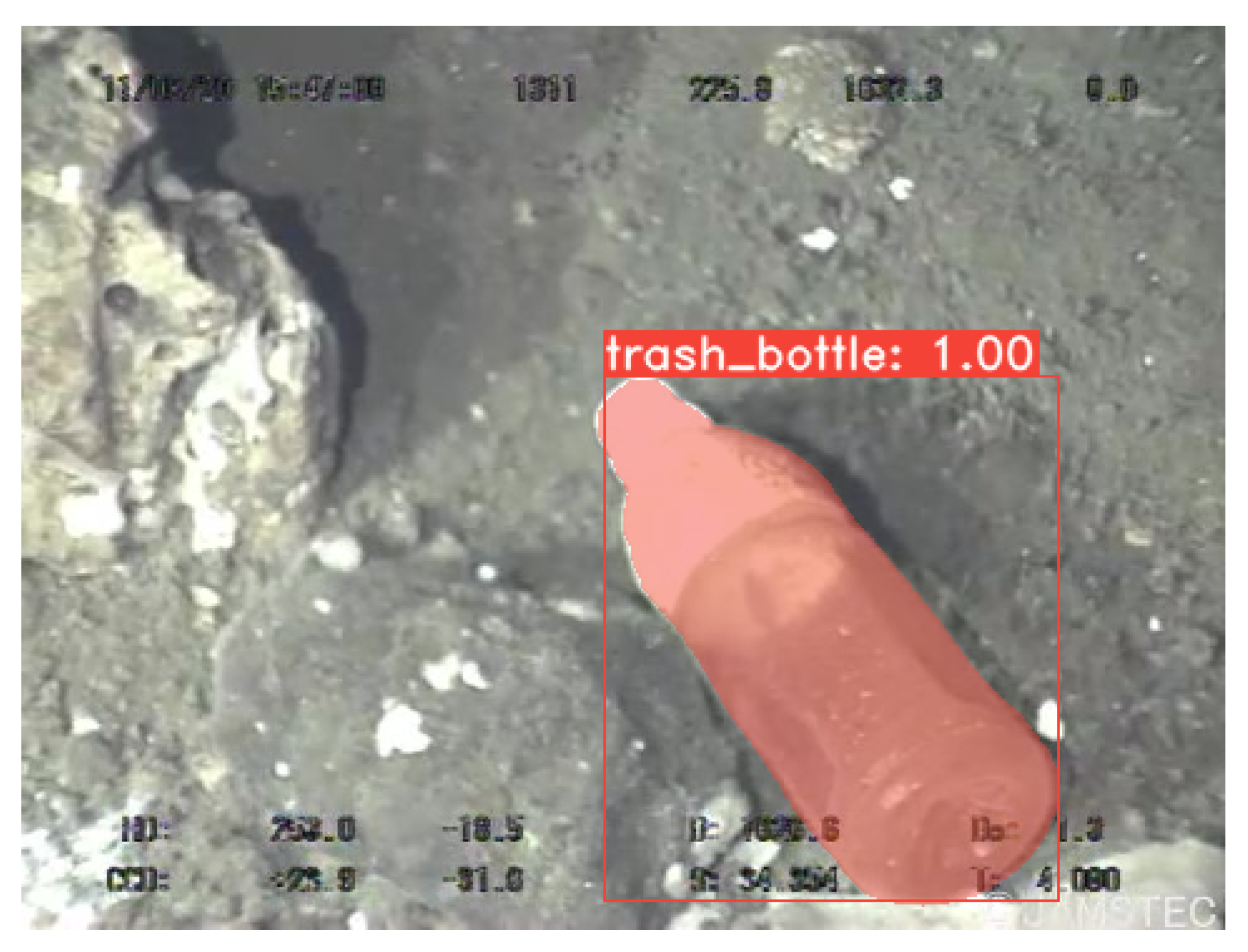
Instance segmentation is a challenging task in computer vision that not only involves detecting objects but also precisely delineating their boundaries at the pixel level, an example of instance segmentation is depicted in Figure 1. Neural-network-based methods have revolutionised instance segmentation, enabling the accurate and efficient segmentation of individual objects within an image.
Several other state-of-the-art techniques have emerged in the field of instance segmentation, each with its unique strengths. One such method is Panoptic FPN, as published in [21], which extends the Mask R-CNN to provide both instance-level and semantic segmentation in a unified framework. By combining instance and semantic segmentation, Panoptic FPN enables a comprehensive understanding of the visual scene. Another noteworthy technique is BlendMask [22], which introduces a new paradigm called BlenderNet for instance segmentation. BlendMask achieves instance segmentation by blending predictions from various feature levels, resulting in highly accurate and detailed segmentations. Furthermore, Segmenting Objects by Locations (SOLO), published in [23], presents an alternative approach to instance segmentation by adopting a fully convolutional framework. SOLO provides the outputs of object masks directly by assigning each pixel to a specific object instance, eliminating the need for a separate post-processing step. This design results in efficient inference and high-quality instance segmentations.
Among the state-of-the-art approaches for instance segmentation, two prominent methods chosen for this paper are YOLACT and the Mask R-CNN. YOLACT, as described in [20], is a real-time instance segmentation method that combines object detection and semantic segmentation. While its primary focus is object detection, YOLACT introduces a novel branch for generating instance-level masks. By leveraging a set of learned coefficients, YOLACT predicts object masks efficiently. This simultaneous detection and segmentation approach makes YOLACT highly efficient and suitable for real-time applications. With its impressive speed and accuracy, YOLACT has established itself as a leading method in instance segmentation. On the other hand, the Mask R-CNN, as described in [24], is another state-of-the-art method, for instance, segmentation that extends the popular Faster R-CNN framework. It combines object detection with pixel-level segmentation, enabling accurate localisation and segmentation of individual objects. The Mask R-CNN employs a backbone network to the R-CNN, typically based on a CNN such as ResNet or VGG, and incorporates two additional subnetworks: a region proposal network (RPN) for generating object proposals and a mask prediction network for generating precise object masks. This multi-stage architecture allows the Mask R-CNN to achieve state-of-the-art performance in instance segmentation. These advancements in instance segmentation will allow for AUVs designed for underwater litter collection to achieve a better sense of the location of the object, thereby allowing for better-automated control of robotic arms in litter collection.
2. Material and Methods
To achieve the goal of detecting marine litter, the overarching procedure involves identifying a suitable dataset, selecting and training an appropriate machine learning model, and then using the trained model to perform image analysis. The quality of the dataset, the capabilities of the model, and the training strategy are crucial factors to consider in this procedure. The details of the computer vision (CV), dataset, and machine learning models will be described in the subsequent sections [25].
2.1. Dataset
Creating a useful trained model requires an adequately diverse dataset that fully represents all of the classes to be analysed [25]. In view of this, the TrashCAN dataset published in [26] was used to train the model, whereby this dataset contains 7212 annotated images that depict underwater trash, ROVs, and undersea flora and fauna. The images are annotated with bitmaps for instance segmentation and contain bounding boxes that surround the instance segments, as shown in Figure 2. The images in the TrashCAN dataset are primarily sourced from the JAMSTEC E-Library of Deep Sea Images (J-EDI) dataset curated by the Japan Agency of Marine Earth Science and Technology (JAMSTEC). The images are extracted from videos taken by ROVs operated by JAMSTEC over the years in the Sea of Japan.
The dataset contains two versions, i.e., instance and material versions, where both use the same set of images, but with different sets of annotations. The instance version focuses on the exact objects depicted in the image, containing classes that include plastic bags, cans, bottles, nets, clothing, and other commonly found trash items. The material version focuses on the material of the trash depicted, with classes for plastic, metal, wood, fabric, and rubber. In both versions of the dataset, the classes for non-trash items such as ROV, flora, and fauna remain the same.
For this study, the instance version of the dataset was chosen to train the models because the intra-class differences in the material version are far too wide to accurately train a useful model. To give an example of the trash classified as plastic, plastic can take on many forms, i.e., plastic bags, six-pack rings, sheets of cling wrap, and plastic household items such as toothbrushes, to name a few. Each of these examples within a single class has vastly different shapes and colours. From the perspective of a model trying to identify plastic, this is a large hurdle to overcome, as the usefulness of the model is highly dependent on the different forms of plastic waste that it will encounter in the dataset. On the other hand, the instance version has a much lower intra-class difference, as the objects described by any given class are restricted to a much more limited set of shapes, with an example being cans or bottles where even if the trash has been damaged or crushed, the object can still be identifiable. Furthermore, if material differentiation is required for application purposes, the instance classes can simply be ascribed to a material type during post-image analysis data processing.
Samples of the images in the TrashCAN dataset, shown in Figure 3, demonstrate some of the difficulties with the image analysis of underwater images. The challenges are mainly attributed to the images with low visibility, visual noise, and the presence of objects of various forms, as described in the following sections.
2.1.1. Low Visibility
The most prominent challenge in image analysis is the low visibility range. As can be seen from the top left image in Figure 3, the depth displayed by the ROV’s video capture system is 2737 m. At this depth, the environment is in a dark condition due to depths below 1000 m receiving no light from the surface (all light seen in the images must be provided by the ROV itself). The range of visibility can be seen in the top right image, i.e., a range of only a few metres. As the ROV gets closer to the object, the range of visibility decreases with the light source nearing the target. This creates a light gradient across the object, as can be seen in the top left image. The suboptimal lighting of underwater imagery primarily affects two factors, i.e., dataset quality and model training time. The dataset must contain the objects in multiple lighting situations to prevent any bias in the results, and by extension, the dataset must be larger as a consequence due to the increased number of lighting scenarios per object. Secondly, it will typically require a larger number of iterations to successfully train the model because of the diverse lighting presentations of any image [26].
2.1.2. Visual Noise
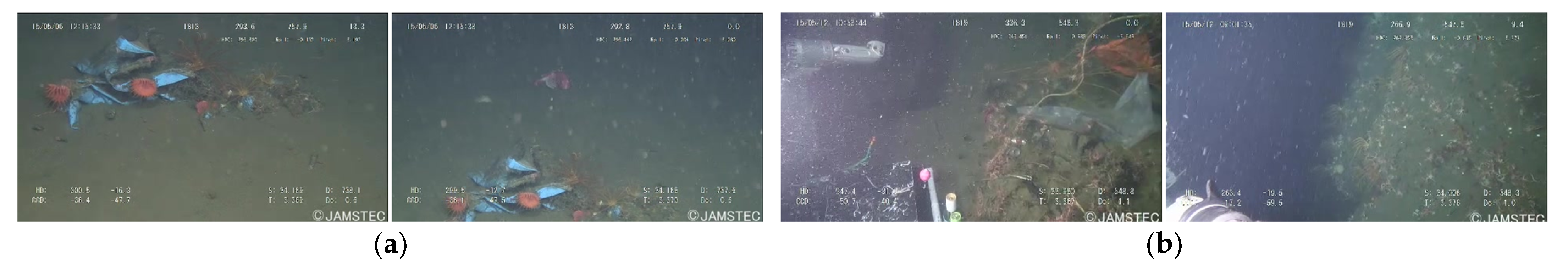
The visual noise caused by floating particles in the water in front of the camera, as shown in Figure 4, may also affect the dataset size and accuracy of the trained model. The noise can mislead or obscure key parts of the object, thereby reducing the accuracy of the model [26]. Figure 4a shows the same object observed in both clear and noisy situations. Figure 4b demonstrates how the strong lighting source aboard an ROV can illuminate suspended particles in the water to create a noisy image.
2.1.3. Objects of Different Forms
Lastly, most objects visible underwater will come in many forms but may be damaged, partially buried, or biofouled. Figure 5a shows cans in different situations, presenting possible distinct designs; they are partially buried and show signs of biofouling. Figure 5b shows three possible forms of plastic bags where their malleable and light nature allows many possible shapes and presentations of the item. With certain shapes, a different angle can show vastly different types of plastics. Figure 5c shows two views of the same object taken several seconds apart as it floats past the stationary ROV. In the left image of Figure 5c, it is viewed with a flat face perpendicular to the camera. In the second image, it is rotated such that its flat face is directly pointing at the camera and presents a distinctly different shape.
Considering the variation in marine litter images, it is key that any dataset used to train the models contains images with a wide array of combinations of the aforementioned situations for similar-looking objects. The TrashCAN dataset contains depictions of objects in the described situations. For model training preparation, the dataset is split into two subsets, i.e., training and validation subsets, using a script provided by [26] in the Microsoft common objects in context (COCO) format. The script randomly distributes the images between the two subsets with an 80–20% split between training and validation. The script also seeks to maintain this ratio as close as possible for all of the classes in the dataset. The split between the different classes can be seen in Table 1.
2.2. Machine Learning Models
To detect marine litter submerged or sunk in the seabed, two models were chosen for training, i.e., the Mask R-CNN and YOLACT. These models use neural networks to parse images and identify objects in them. However, they take different approaches, where these approaches affect their computational requirements and their accuracy. Two metrics were used in evaluating the accuracy of the models, i.e., the mean average precision () and intersection over union (IoU). The details of the Mask R-CNN and YOLACT will be described in the subsequent subsections.
2.2.1. The Mask R-CNN
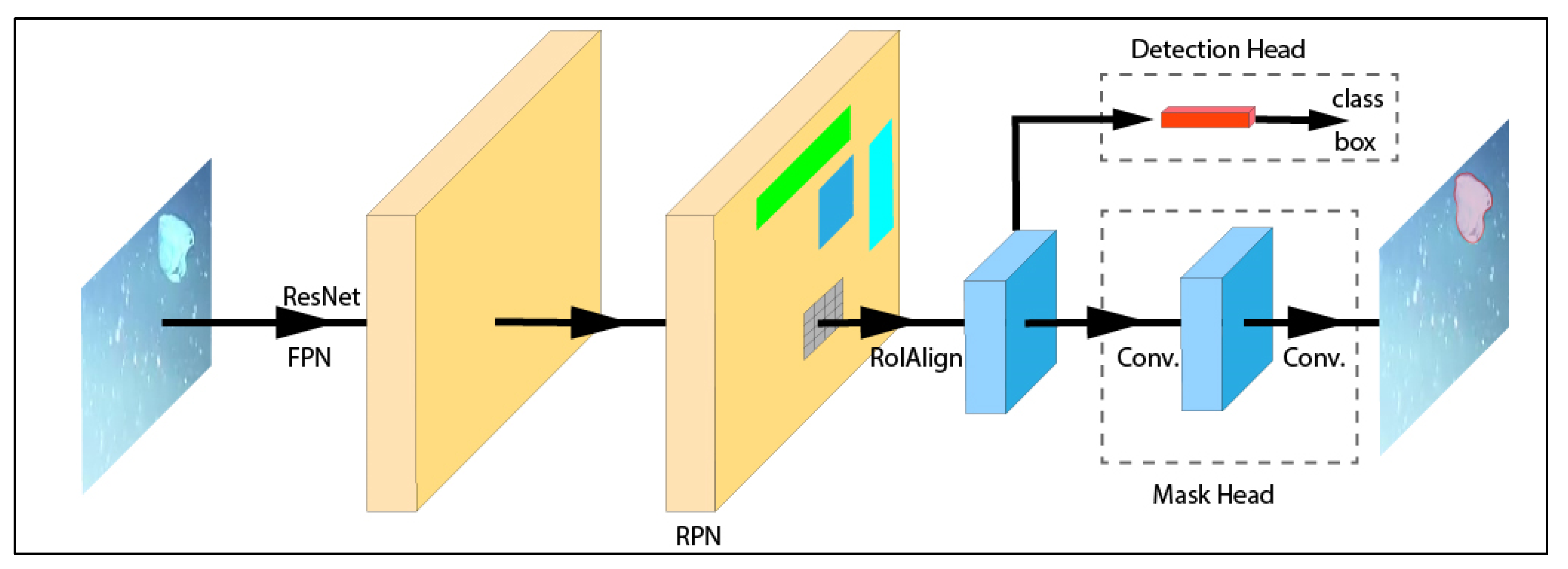
The Mask R-CNN is a neural-network-based object instance segmentation framework extended from the Faster R-CNN [26]. It was first published in [24] and has the capability to predict object masks (i.e., detection and segmentation) in parallel to the classification capabilities of the Faster R-CNN. The detection and segmentation tasks by the Mask R-CNN framework are carried out in the mask head, whereas the classification task by the original Faster R-CNN is executed in the detection head, as shown in Figure 6.
The Mask R-CNN uses the RolAlign operation in extracting a small feature map from each RoI in the detection and segmentation tasks. The Mask R-CNN executes a parallel mask branch (mask head), which is a small fully convolutional network (FCN), for predicting segmentation masks in each region of interest (RoI) through pixel-wise segmentation mask prediction. It allows for pixel-to-pixel alignment and the preservation of spatial location by foregoing quantisation during the RoI detection step. On the other hand, the original Faster R-CNN (denoted as the detection head in Figure 6) performs the bounding box and classification regression. After both branches were complete, the data from the classification branch were combined with the main segmentation branch to assign a class to the object mask. The additional mask branch presents a small computational overhead to the Faster R-CNN. However, it is noted that the Mask R-CNN is still limited by the speed of the first FCN in the model [24].
When this research was conducted, the Mask R-CNN outperformed all of the other single-model instance segmentation solutions trained on Microsoft’s COCO dataset, as reported in [23]. It serves as a benchmark for instance segmentation models and, for this paper, served as a baseline to YOLACT. The primary benefit of using the Mask R-CNN is its accuracy. However, this accuracy comes at a price, i.e., the Mask R-CNN is a very heavyweight model that uses a large amount of memory during both training and usage. It processes images at a rate of 5 frames per second (fps), even though it was run on a Nvidia Tesla M40 GPU, a high-performance GPU [24]. It is noted that 5 fps is too slow for real-time applications, as real-time image analysis is generally considered to be at speeds of 30 fps or greater [20]. The slow speed of the Mask R-CNN, therefore, limits it to the post-capture analysis of videos and images with the advantage of higher accuracy.
2.2.2. YOLACT
YOLACT is an architecture that can perform real-time instance segmentation. YOLACT takes inspiration from models such as YOLO and Single-Shot Detectors (SSD) that use single-stage bounding box object detection to give them advantages over the Mask R-CNN’s two-stage architecture [20]. Furthermore, instance segmentation used in the Mask R-CNN is a much more complex task than bounding box detection used in YOLACT. As shown in Figure 6, the Mask R-CNN is an inherently sequential task as it uses a two-stage instance segmentation model. Thus, it depends on feature localisation to produce object masks by repooling bounding box features to feed them into a mask detection layer; see Figure 6.
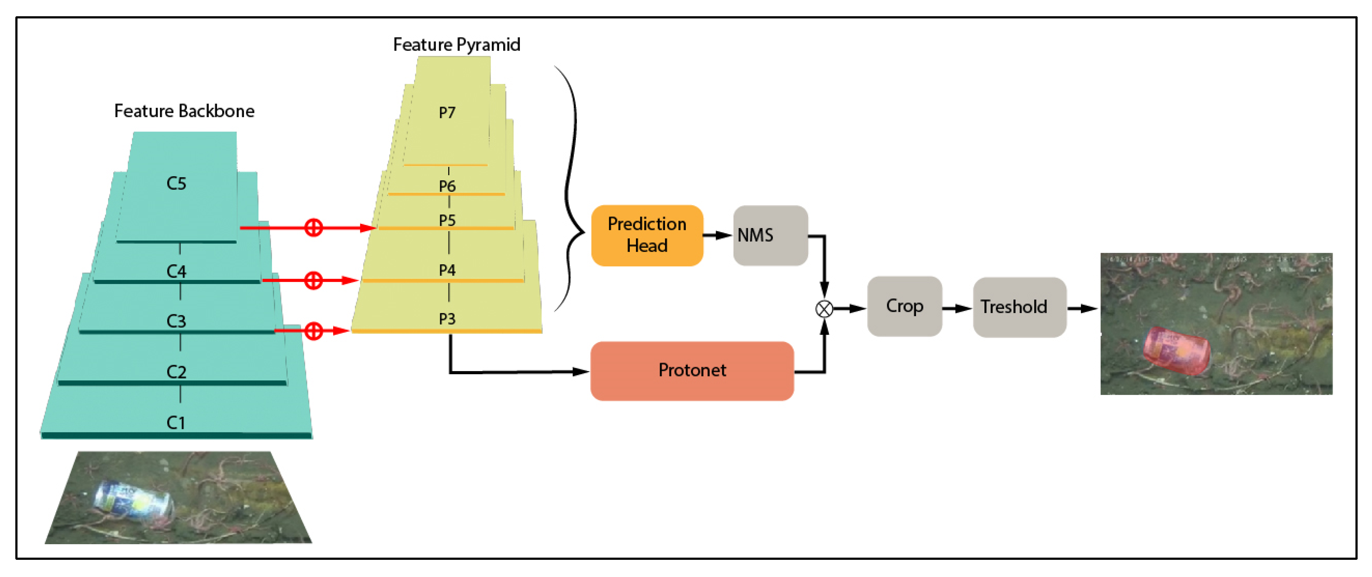
To circumvent the inherent difficulty of optimisation, YOLACT removes an explicit localisation step using two parallel tasks to perform instance segmentation, as shown in Figure 7. The first task is to generate a set of non-local prototype masks in the Protonet step over the entire image, whereas the second task is to predict a set of linear combination coefficients per instance. Instance segmentation is then performed by linearly combining the prototype masks with the predicted coefficients in each instance. Through this process, the neural network can localise the masks instead of using an explicit step to do so, as in the Mask R-CNN.
The parallel stages allow for greatly increased speed over traditional two-step approaches, with capabilities of processing images at an fps greater than 30. This does come with a minor drop in accuracy, but it is still capable of producing competitive results [20].
2.3. Training
One key aspect of instance segmentation training is that it requires an extremely large dataset to train on, i.e., greater than 100k images. However, the TrashCAN dataset is not large enough to fully train a model from scratch. The common solution to this problem is to take advantage of transfer learning, as shown in Figure 8. Transfer learning makes use of a pre-trained model that has already been fully trained on a general dataset. This pre-trained model contains the weights to differentiate objects from the background, distinguish one object from another, and identify individual overlapping objects. To train on a smaller dataset, the bottom layers of the pre-trained model are locked while keeping the top few layers unlocked. The top layers are then trained on the dataset, refining the pre-trained model to the dataset as desired [28].
In this paper, both the Mask R-CNN and YOLACT models were trained on dual Nvidia RTX A4000 GPUs. It is important to note that the optimal iterations and learning rate for YOLACT were calculated differently to the Mask R-CNN and that both models were trained to completion while avoiding overfitting.
2.3.1. Mask R-CNN
The implementation used to train the Mask R-CNN in this paper followed the method given by Ahmed Gad [29]. It replicates the Mask R-CNN architecture in [24] but is implemented in Google’s Tensorflow 2.2. The implementation by Ahmed Gad [29] is an adaptation of the implementation created by Matterport for Tensorflow 1.0 [30]. The model is trained from model weights that are pre-trained on the COCO2017 dataset using a ResNet101 backbone. When training the model, the bottom four ResNet stages are locked, except when fine-tuning the model. The model is trained at a learning rate of 0.001 and is reduced by a factor of 10 when fine-tuning. The Mask R-CNN model resizes images to 1024 × 1024 pixels and images that are not square are padded with black bars. The training runs for 40,000 iterations but begins to overfit at 30,000 iterations. So, the model version at 30,000 iterations was used for evaluation.
2.3.2. YOLACT
The implementation used to train the YOLACT model in this paper followed the technique given in [20]. Like the Mask R-CNN, it is also trained from model weights that are pre-trained on the COCO2017 dataset. A ResNet101 backbone is also used for this model. During training, the bottom layer of the prototype mask generator is locked. The model is trained with a learning rate of 0.001, with the learning rate being reduced by a factor of 10 at 280,000, 360,000, and 400,000 iterations, respectively. Images are resized to 550 × 550 pixels for training without maintaining the aspect ratio. During the evaluation, the images are resized to 550 × 550 pixels, and then the generated masks are upscaled to match the full-size image. The training is stopped at 452,000 iterations when the model begins to overfit.
2.4. Evaluation
Both the Mask R-CNN and YOLACT models were trained and evaluated on the same training and validation set. The evaluation was conducted using the standard COCO style metrics of average precision () at different intersections over union (IoU) thresholds. The incorporates three key values, i.e., IoU, precision and recall, as described in the following sections.
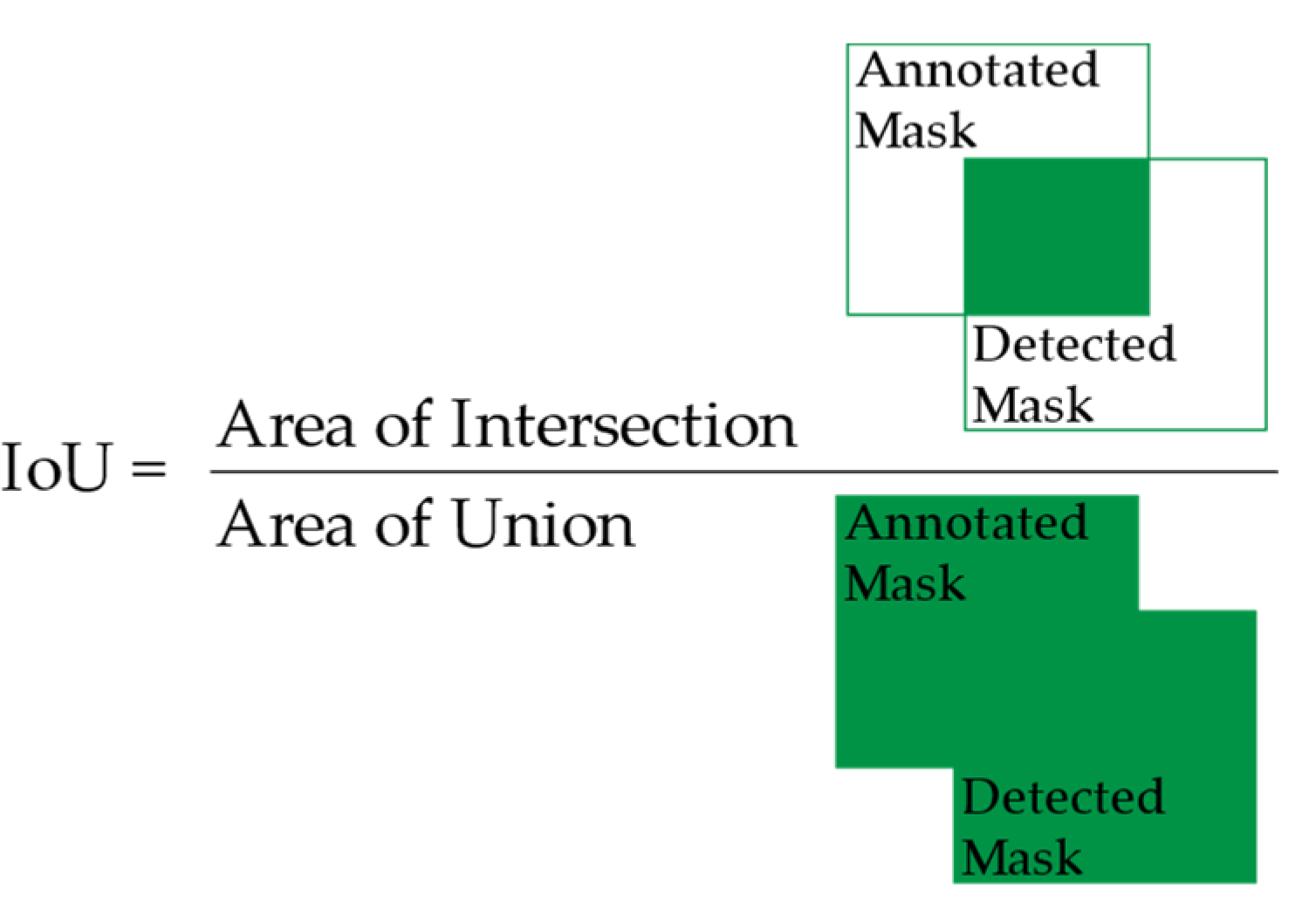
2.4.1. Intersection over Union (IoU)
The calculation for IoU is shown in Figure 9 for the case of instance segmentation. The IoU is obtained by dividing the area of intersection by the area of union, as shown where the area of intersection is the intersection between the pixels bounded by the annotated mask and detected mask, whereas the area of union is the union between the pixels of both aforementioned masks. A high IoU (close to 1.0) indicates a predicted mask closely resembling the annotated mask. Using the IoU metric allows evaluators to distinguish between four types of results, i.e., true positives, true negatives, false positives, and false negatives. A predicted mask with a different class to the annotated mask would have an IoU of 0.0, as there would be no overlapping.
2.4.2. Precision (P)
The precision is calculated as follows,
where denotes precision, denotes the true positives, and denotes the false positives. Precision is calculated with an IoU threshold. For example, with an IoU threshold of 0.5, a predicted mask with an IoU of 0.8 would be considered as a true positive, while a mask with an IoU of 0.4 will be considered as a false positive. It is to be noted that AP does not equate to the mean of precisions. The calculation for AP involves an additional metric, i.e., recall.
2.4.3. Recall (R)
Recall is a metric that describes the ratio between and all predictions, given as
where denotes recall, denotes the true positives, and denotes the false negatives. Precision and recall are then plotted on a curve using each IoU threshold ranging from 0.0 to 1.0, as shown in Figure 10.
2.4.4. Accuracy Metrics—Average Precision () and Mean Average Precision ()
To calculate average precision for a given IoU threshold, the area under the curve in Figure 10, up to the desired threshold, is calculated as
where is the IoU threshold and is the upper limit of the IoU threshold. Equation (3) shows that a high IoU threshold will result in a lower score as it will take a smaller area under the curve.
Once the has been obtained, the is calculated. The is a metric proposed in the COCO2017 Evaluation Challenge which has ten IoU thresholds ranging from 0.50 to 0.95, with a step size of 0.05. To calculate , the must first be calculated for each class, at each IoU threshold, and then the average of all classes at all thresholds is taken. This typically results in an of approximately 0.30 for a model well-trained on the COCO dataset. The reason it seems so low is that the COCO dataset is a complex dataset with over 80 classes [27].
When evaluating the model in this paper, the evaluation was run on two differently performing GPUs, i.e., the higher-performing Nvidia Quadro A4000 and the lower-performing Nvidia GTX 1050 Ti, for a comparison between a machine-learning-optimised GPU and a lower-power GPU. Both evaluations arrived at similar results, as they used the same model weights and the same validation set. The only difference between the two evaluations was the computational time taken. This shows that a lower-power and less-costly GPU could be placed on board an ROV for image detection without much loss in accuracy.
3. Results
3.1. Qualitive Analysis
The sample results comparing both the Mask R-CNN and YOLACT models are presented in Figure 11. The predicted masks are denoted by the rectangular bounding boxes in each image. The images in Figure 11 show that the masks and classification are similar, but with some key differences. The masks generated by the Mask R-CNN are more irregular (denoted by the uneven borders in Figure 11a,b) when compared to the counterparts generated by YOLACT, and do not necessarily cover the entire object; hence, they show a slightly lower IoU. This can be tied back to the pre-trained model and how it interacts with transfer learning. The pre-trained models for both the Mask R-CNN and YOLACT were trained on COCO2017, which has many classes. However, most of the images in the COCO2017 dataset show relatively good lighting and were taken during the daytime. In the present case, the worst lighting conditions of the TrashCAN dataset present a challenge for the sequential architecture of the Mask R-CNN.
The lack of clarity around the edges of the mask generated by lower light levels is likely caused by the RoIAlign layer not being able to accurately localise RoIs. This is because the RoIAlign layer is locked during training, which results in the mask layer ‘looking in the wrong place’ by the time it gets to the mask generation step. On the other hand, YOLACT, which lacks an explicit feature localisation step, can circumvent this issue, as any errors in the prototype mask generator due to the lower light levels can be lightly corrected when combined with the linear combination coefficients in the last step, as shown in Figure 7 [20]. To improve the mask accuracy of the Mask R-CNN with the existing pre-trained weights, it is likely that it would require modification to the architecture of the RoIAlign step for it to account for softer edges on objects caused by low light levels. An alternative solution to this issue is to make use of a pre-trained model that has been trained on lower-light-level images. The optimal solution would be to have a model trained exclusively on underwater images.
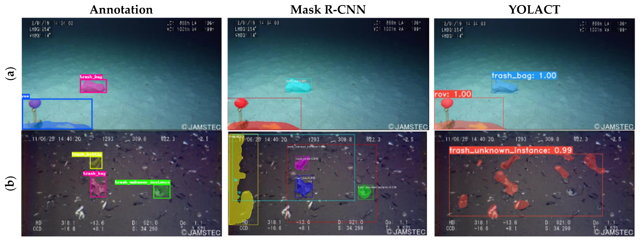
Figure 12 demonstrates the differences in classification between YOLACT and the Mask R-CNN. The Mask R-CNN can detect the individual instances and label them correctly, whereas YOLACT classifies all objects as large unknown instances. Another thing to note is that in the Mask R-CNN’s detection, there is an additional instance (highlighted in yellow in Figure 12b) that is detected but not included in the annotations. When detecting across the dataset, this type of ‘phantom’ detection around the border of the image is occasional and typically occurs in images with darker borders, such as the one found in Figure 12. The likely cause of this is the large number of images in the dataset with portions of the ROV visible, or cases where the ROV parts are partially obscured by the low light level. This can be mitigated by enriching the dataset using image augmentation of the original images by reducing the proportion of images containing the ROV.
3.2. Quantitative Analysis
3.2.1. Comparison between Mask R-CNN and YOLACT
The performance of the Mask R-CNN and YOLACT in accurately classifying marine underwater litter from the TrashCAN dataset is summarised in Table 2.
The metric was used to evaluate the performance of the models. The results show that the Mask R-CNN outperforms YOLACT in the accuracy metrics, as the Mask R-CNN is a much more computationally expensive model. YOLACT’s lightweight structure using the parallel stages of mask prototypes and coefficients is more limited by the implied nature of its calculation. However, it is interesting to note that both models outperformed their pre-trained models’ performance on the COCO dataset. The of the original pre-trained model weights on the COCO dataset is widely considered to be the most cutting-edge in general-use instance segmentation [20]. Achieving metrics that exceed those of the pre-trained weights in a specialised dataset can be explained by the fact that the TrashCAN dataset has considerably fewer classes than the COCO dataset. Therefore, the model has fewer possibilities of incorrectly classifying an object as the wrong class, thus improving its .
The difference in the speed of the models is also clearly seen in Table 3. With YOLACT taking advantage of its parallel stages, it is capable of being over three times faster on the lower-end GPU and six times faster on a machine-learning-optimised GPU, while only trading off a comparatively smaller amount of accuracy. The difference in the increased speed of YOLACT between the two GPUs is likely a result of differing bottlenecks between the two GPUs.
3.2.2. Comparison to Other Models
The two models studied in this paper were compared to other published results of models trained on the TrashCAN dataset as shown in Table 4. The accuracy results of the present method are in line with previously published results, particularly in terms of the metric. These publications did not publish data about the speed of the trained models, but it can be inferred that they would have similar speeds to the Mask R-CNN results of this paper.
It is worth noting that there are limited published results that meet the requirements for a fair comparison to the results published in this paper. The majority of existing publications study the object detection of many types of marine litter, i.e., shore and floating, and only a handful are related to instance segmentation models on underwater litter [19].
4. Conclusions
This paper presented two different instance segmentation methodologies for the detection of marine underwater litter, i.e., YOLACT and the Mask R-CNN. YOLACT, being a lightweight model that can run quickly on lower-end hardware, has the potential to be deployed in a fleet of smart AUVs for the automated collection of marine litter. The low computational power requirement in YOLACT requires less costly hardware and a lower energy requirement, thereby prolonging the battery life and allowing longer litter detection duration in real-time. On the other hand, the study from the Mask R-CNN showed a higher , thus indicating higher accuracy in marine litter detection. The Mask R-CNN is more suitable to be used in surveying. The high computational requirements of the Mask R-CNN can be overcome by processing the imagery on a land-based data centre, where parallel computing can be used to increase the effective frame rate. The Mask R-CNN has an advantage over YOLACT as it allows for trawling, which is an indiscriminate process to detect marine flora and fauna. With the detection of marine flora and fauna, these populations can be protected during the clean-up process. The instance segmentation techniques presented in this paper served as an important step in cleaning up the ocean, as the results shown by YOLACT and the Mask R-CNN are promising and can be used in marine litter clean-up. Future research with larger datasets and better-optimised models will be able to achieve more accurate results.
Author Contributions
Conceptualisation, B.C.C.; methodology, B.C.C.; validation, B.C.C.; writing—original draft preparation, B.C.C.; data collection: B.C.C.; writing—review and editing, Z.Y.T.; visualisation, B.C.C. and Z.Y.T.; supervision, Z.Y.T. and D.K.; project administration, Z.Y.T.; funding acquisition, Z.Y.T. and D.K. All authors have read and agreed to the published version of the manuscript.
Funding
This research was funded by MOE, grant number R-MOE-E103-F010.
Data Availability Statement
The dataset analysed in this study is openly available at https://doi.org/10.13020/g1gx-y834 (accessed on 29 May 2023).
Conflicts of Interest
The funders had no role in the design of the study; in the collection, analyses, or interpretation of data; in the writing of the manuscript; or in the decision to publish the results.
References
- National Geographic Society. Why the Ocean Matters. 2023. Available online: https://education.nationalgeographic.org/resource/why-ocean-matters/ (accessed on 9 June 2023).
- National Geographic Society. Ocean Trash: 5.25 Trillion Pieces and Counting, but Big Questions Remain. 2022. Available online: https://education.nationalgeographic.org/resource/ocean-trash-525-trillion-pieces-and-counting-big-questions-remain/ (accessed on 9 June 2023).
- United Nations Statistics Division. Conserve and Sustainably Use the Oceans, Sea and Marine Resources for Sustainable Development. 2022. Available online: https://unstats.un.org/sdgs/report/2022/Goal-14/ (accessed on 9 June 2023).
- Sharma, S.; Sharma, V.; Chatterjee, S. Microplastics in the Mediterranean Sea: Sources, Pollution Intensity, Sea Health, and Regulatory Policies. Front. Mar. Sci. 2021, 8, 494. [Google Scholar] [CrossRef]
- Alabi, O.A.; Ologbonjaye, K.I.; Awosolu, O.; Alalade, O.E. Public and Environmental Health Effects of Plastic Wastes Disposal: A Review. J. Toxicol. Risk Assess. 2019, 5, 1–13. [Google Scholar] [CrossRef]
- Gallo, F.; Fossi, C.; Weber, R.; Santillo, D.; Sousa, J.; Ingram, I.; Nadal, A.; Romano, D. Marine litter plastics and microplastics and their toxic chemicals components: The need for urgent preventive measures. Environ. Sci. Eur. 2018, 30, 13. [Google Scholar] [CrossRef] [PubMed]
- Newman, S.; Watkins, E.; Farmer, A.; Brink, P.T.; Schweitzer, J.P. The economics of marine litter. Mar. Anthropog. Litter 2015, 367–394. [Google Scholar] [CrossRef] [Green Version]
- Pabortsava, K.; Lampitt, R.S. High concentrations of plastic hidden beneath the surface of the Atlantic Ocean. Nat. Commun. 2020, 11, 4073. [Google Scholar] [CrossRef] [PubMed]
- Voyer, M.; Schofield, C.; Azmi, K.; Warner, R.; McIlgorm, A.; Quirk, G. Maritime security and the Blue Economy: Intersections and interdependencies in the Indian Ocean. J. Indian Ocean Reg. 2017, 14, 28–48. [Google Scholar] [CrossRef] [Green Version]
- Maes, T.; Barry, J.; Leslie, H.A.; Vethaak, A.D.; Nicolaus, E.E.M.; Law, R.; Lyons, B.P.; Martinez, R.; Harley, B.; Thain, J.E. Below the surface: Twenty-five years of seafloor litter monitoring in coastal seas of North West Europe (1992–2017). Sci. Total Environ. 2018, 630, 790–798. [Google Scholar] [CrossRef] [PubMed]
- Pham, C.K.; Ramirez-Llodra, E.; Alt, C.H.S.; Amaro, T.; Bergmann, M.; Canals, M.; Company, J.B.; Davies, J.; Duineveld, G.; Galgani, F.; et al. Marine Litter Distribution and Density in European Seas, from the Shelves to Deep Basins. PLoS ONE 2014, 9, e95839. [Google Scholar] [CrossRef] [PubMed] [Green Version]
- Schwarz, A.; Ligthart, T.; Boukris, E.; van Harmelen, T. Sources, transport, and accumulation of different types of plastic litter in aquatic environments: A review study. Mar. Pollut. Bull. 2019, 143, 92–100. [Google Scholar] [CrossRef] [PubMed]
- Valdenegro-Toro, M. Submerged marine debris detection with autonomous underwater vehicles. In Proceedings of the 2016 International Conference on Robotics and Automation for Humanitarian Applications (RAHA), Kollam, India, 18–20 December 2016; pp. 1–7. [Google Scholar] [CrossRef]
- Madricardo, F.; Ghezzo, M.; Nesto, N.; Mc Kiver, W.J.; Faussone, G.C.; Fiorin, R.; Riccato, F.; Mackelworth, P.C.; Basta, J.; De Pascalis, F.; et al. How to Deal with Seafloor Marine Litter: An Overview of the State-of-the-Art and Future Perspectives. Front. Mar. Sci. 2020, 7, 830. [Google Scholar] [CrossRef]
- Tudor, D.T.; Williams, A.T. Marine Debris-Onshore, Offshore, and Seafloor Litter. In Encyclopedia of Coastal Science; Springer: Amsterdam, The Netherlands, 2019; pp. 1125–1129. [Google Scholar] [CrossRef]
- Erbe, C.; Duncan, A.; Vigness-Raposa, K.J. Introduction to Sound Propagation Under Water. In Exploring Animal Behavior Through Sound; Springer: Berlin/Heidelberg, Germany, 2022; Volume 1, pp. 185–216. [Google Scholar]
- Spengler, A.; Costa, M.F. Methods applied in studies of benthic marine debris. Mar. Pollut. Bull. 2008, 56, 226–230. [Google Scholar] [CrossRef] [PubMed]
- Ardana, I.W.R.; Purnama, I.B.I.; Yasa, I.M.S. Application of Object Recognition for Plastic Waste Detection and Classification Using YOLOv3. In Proceedings of the 3rd International Conference on Applied Science and Technology, iCAST 2020, Padang, Indonesia, 24–25 October 2020; pp. 652–656. [Google Scholar] [CrossRef]
- Jia, T.; Kapelan, Z.; de Vries, R.; Vriend, P.; Peereboom, E.C.; Okkerman, I.; Taormina, R. Deep learning for detecting macroplastic litter in water bodies: A review. Water Res. 2023, 231, 119632. [Google Scholar] [CrossRef] [PubMed]
- Bolya, D.; Fanyi, C.Z.; Yong, X.; Lee, J. YOLACT Real-Time Instance Segmentation. 2019. Available online: https://github.com/dbolya/yolact (accessed on 16 July 2022).
- Kirillov, A.; Girshick, R.; He, K.; Dollár, P. Panoptic feature pyramid networks. In Proceedings of the IEEE/CVF Conference on Computer Vision and Pattern Recognition, Long Beach, CA, USA, 15–20 June 2019; pp. 6399–6408. [Google Scholar] [CrossRef] [Green Version]
- Chen, H.; Sun, K.; Tian, Z.; Shen, C.; Huang, Y.; Yan, Y. BlendMask: Top-Down Meets Bottom-Up for Instance Segmentation. In Proceedings of the IEEE Computer Society Conference on Computer Vision and Pattern Recognition, Seattle, WA, USA, 13–19 June 2020; pp. 8570–8578. [Google Scholar] [CrossRef]
- Wang, X.; Zhang, R.; Shen, C.; Kong, T.; Li, L. SOLO: A Simple Framework for Instance Segmentation. IEEE Trans. Pattern Anal. Mach. Intell. 2021, 44, 8587–8601. [Google Scholar] [CrossRef] [PubMed]
- He, K.; Gkioxari, G.; Dollár, P.; Girshick, R. Mask R-CNN. IEEE Trans. Pattern Anal. Mach. Intell. 2017, 42, 386–397. [Google Scholar] [CrossRef] [PubMed]
- Gong, Z.; Zhong, P.; Hu, W. Diversity in Machine Learning. IEEE Access 2019, 7, 64323–64350. [Google Scholar] [CrossRef]
- Hong, J.; Fulton, M.; Sattar, J. TrashCan: A Semantically-Segmented Dataset towards Visual Detection of Marine Debris (Preprint). 2020. Available online: https://www.researchgate.net/publication/343005360_TrashCan_A_Semantically-Segmented_Dataset_towards_Visual_Detection_of_Marine_Debris (accessed on 22 June 2023).
- Deng, H.; Ergu, D.; Liu, F.; Ma, B.; Cai, Y. An Embeddable Algorithm for Automatic Garbage Detection Based on Complex Marine Environment. Sensors 2021, 21, 6391. [Google Scholar] [CrossRef] [PubMed]
- Weiss, K.; Khoshgoftaar, T.M.; Wang, D.D. A survey of transfer learning. J. Big Data 2016, 3, 1345–1459. [Google Scholar] [CrossRef] [Green Version]
- GitHub—Ahmedfgad/Mask-RCNN-TF2: Mask R-CNN for Object Detection and Instance Segmentation on Keras and TensorFlow 2.0. Available online: https://github.com/ahmedfgad/Mask-RCNN-TF2 (accessed on 17 July 2022).
- GitHub—Matterport/Mask_RCNN: Mask R-CNN for Object Detection and Instance Segmentation on Keras and TensorFlow. Available online: https://github.com/matterport/Mask_RCNN (accessed on 17 July 2022).
- Kurbiel, T. Gaining an Intuitive Understanding of Precision, Recall and Area Under Curve|by Thomas Kurbiel|Towards Data Science. 2020. Available online: https://towardsdatascience.com/gaining-an-intuitive-understanding-of-precision-and-recall-3b9df37804a7 (accessed on 18 July 2022).
Figure 1.
Instance segmentation example using YOLACT with the IoU metric.

Figure 2.
Example of TrashCAN dataset showing bounding boxes and mask annotations.

Figure 3.
Sample of images from TrashCAN [26].
Figure 3.
Sample of images from TrashCAN [26].

Figure 4.
Images with visual noise. (a) The same object in a clear and noisy observation. (b) Example of the strong light source aboard the ROV creating noise from suspended particles.
Figure 4.
Images with visual noise. (a) The same object in a clear and noisy observation. (b) Example of the strong light source aboard the ROV creating noise from suspended particles.

Figure 5.
Objects in different situations. (a) Three different variations of a can. (b) Different shapes of plastic bags. (c) The same object is from two angles with a vastly different apparent shape.
Figure 5.
Objects in different situations. (a) Three different variations of a can. (b) Different shapes of plastic bags. (c) The same object is from two angles with a vastly different apparent shape.

Figure 6.
The Mask R-CNN framework showing the parallel second stage [27].
Figure 6.
The Mask R-CNN framework showing the parallel second stage [27].

Figure 7.
YOLACT architecture [20].
Figure 7.
YOLACT architecture [20].

Figure 8.
Transfer learning.

Figure 9.
Graphic depicting IoU.

Figure 10.
Precision–recall curve [31].
Figure 10.
Precision–recall curve [31].

Figure 11.
Sampled results comparing both models displaying the class and IoU of the predicted mask (Mask R-CNN labels have been overlayed for better viewing (a–c), YOLACT models: (d–f)).
Figure 11.
Sampled results comparing both models displaying the class and IoU of the predicted mask (Mask R-CNN labels have been overlayed for better viewing (a–c), YOLACT models: (d–f)).

Figure 12.
Comparison between the annotated mask and the detected mask for selected images. (a) Example image of a singular plastic bag in the image. (b) Example image with multiple objects.
Figure 12.
Comparison between the annotated mask and the detected mask for selected images. (a) Example image of a singular plastic bag in the image. (b) Example image with multiple objects.


Table 1.
Split of training (Train) and validation (Val) subsets.
| Class Name | Train Instances | Validation Instances | Total Instances | Ratio (Train–Val) |
|---|---|---|---|---|
| animal_crab | 246 | 63 | 309 | 0.80–0.20 |
| animal_eel | 259 | 84 | 343 | 0.76–0.24 |
| animal_etc | 170 | 65 | 235 | 0.72–0.28 |
| animal_fish | 611 | 153 | 764 | 0.80–0.20 |
| animal_shells | 188 | 61 | 249 | 0.76–0.24 |
| animal_starfish | 262 | 136 | 398 | 0.66–0.34 |
| plant | 405 | 102 | 507 | 0.80–0.20 |
| rov | 2633 | 684 | 3447 | 0.76–0.20 |
| trash_bag | 727 | 181 | 910 | 0.80–0.20 |
| trash_bottle | 100 | 26 | 126 | 0.79–0.21 |
| trash_branch | 268 | 68 | 336 | 0.80–0.20 |
| trash_can | 366 | 93 | 461 | 0.79–0.20 |
| trash_clothing | 65 | 17 | 82 | 0.79–0.21 |
| trash_container | 407 | 103 | 510 | 0.80–0.20 |
| trash_cup | 47 | 12 | 59 | 0.80–0.20 |
| trash_net | 94 | 33 | 130 | 0.72–0.25 |
| trash_pipe | 114 | 42 | 156 | 0.73–0.27 |
| trash_rope | 88 | 29 | 117 | 0.75–0.25 |
| trash_snack_wrapper | 67 | 17 | 84 | 0.80–0.20 |
| trash_tarp | 90 | 31 | 122 | 0.74–0.25 |
| trash_unknown_instance | 2203 | 553 | 2761 | 0.80–0.20 |
| trash_wreckage | 130 | 35 | 165 | 0.79–0.21 |
Table 2.
Instance segmentation evaluation results.
| Property | Mask R-CNN | YOLACT |
|---|---|---|
| Backbone | ResNet-101 | Resnet-101 |
| 𝒎𝑨𝑷 | 0.377 | 0.365 |
| 0.588 | 0.563 | |
| 0.425 | 0.413 | |
| 0.103 | 0.096 | |
| of pre-trained weights on COCO2017 evaluation | 0.361 | 0.298 |
Table 3.
Speed comparison of both models on two graphic cards.
| GPU | Mask R–CNN | YOLACT |
|---|---|---|
| Nvidia GTX 1050 Ti (lower-end GPU) | 1.6 FPS | 5.1 FPS |
| Nvidia Quadro P4000 (higher-end GPU) | 6.1 FPS | 41.2 FPS |
Disclaimer/Publisher’s Note: The statements, opinions and data contained in all publications are solely those of the individual author(s) and contributor(s) and not of MDPI and/or the editor(s). MDPI and/or the editor(s) disclaim responsibility for any injury to people or property resulting from any ideas, methods, instructions or products referred to in the content. |
© 2023 by the authors. Licensee MDPI, Basel, Switzerland. This article is an open access article distributed under the terms and conditions of the Creative Commons Attribution (CC BY) license (https://creativecommons.org/licenses/by/4.0/).
Share and Cite
MDPI and ACS Style
Corrigan, B.C.; Tay, Z.Y.; Konovessis, D. Real-Time Instance Segmentation for Detection of Underwater Litter as a Plastic Source. J. Mar. Sci. Eng. 2023, 11, 1532. https://doi.org/10.3390/jmse11081532
AMA Style
Corrigan BC, Tay ZY, Konovessis D. Real-Time Instance Segmentation for Detection of Underwater Litter as a Plastic Source. Journal of Marine Science and Engineering. 2023; 11(8):1532. https://doi.org/10.3390/jmse11081532
Chicago/Turabian StyleCorrigan, Brendan Chongzhi, Zhi Yung Tay, and Dimitrios Konovessis. 2023. "Real-Time Instance Segmentation for Detection of Underwater Litter as a Plastic Source" Journal of Marine Science and Engineering 11, no. 8: 1532. https://doi.org/10.3390/jmse11081532
Note that from the first issue of 2016, this journal uses article numbers instead of page numbers. See further details here.