A Numerical Study on the Hydrodynamic Performance of a Tanker in Bow Sea Conditions Depending on Restraint Conditions

Abstract

The importance of accurate ship performance estimation is increasing for efficient ship operation. Ship performance has been evaluated through model tests in the past, but there are limitations in terms of facilities and costs. With the spread of high-performance computers, the method of evaluating the performance of a ship by numerical analysis, especially computational fluid dynamics (CFD), has become common. There have been many numerical studies on added resistance under various wave conditions for many years, showing a high reliability. Meanwhile, most of the studies were conducted under conditions where the degree of freedom (DOF) of the ship was limited due to computational complexity. In this study, we tried to compare the added resistance performance and fluid dynamics of S-VLCC with 6 DOFs in the regular wave conditions. One of the methods for utilizing the 6 DOFs is the soft-mooring system, which allows springs to be attached to the bow and stern to recover the non-restoring force of the hull. The second method considers the free-running condition. The virtual disk is used for the self-propulsion of the ship, and the rudder can be rotated to maintain its course. The propeller rotation speed and rudder angle are controlled through PID control. The bow wave (ψ = 180°) and oblique wave (ψ = 150°, 120°) conditions were considered, and various regular wave conditions from short to long wavelengths were regarded. The effects of restraint conditions on the added resistance and motion response amplitude operator (RAO), according to each wave condition, were compared. As a result, there was a difference in the roll motion for each restraint condition, and the y-direction force and yaw moment generated on the hull were compared to analyze the cause. In addition, we observed the change in flow characteristics by comparing the streamlines around the hull and the nominal wake on the propeller plane.

1. Introduction

Efforts to enhance ship performance are intensifying as environmental regulations for ships become more stringent. To estimate ship performance in general, the resistance required for a ship to advance at a constant speed is measured, and the effective horsepower (EHP) is calculated in the calm water condition. On the other hand, Vinayak et al. [1] showed that there are various sea conditions by a real seaway through worldwide oceanic wind and wave data on the ECMWF website. It was pointed out that a large difference occurred by comparing the travel time and fuel consumption according to sea conditions in the same vessel.

Real-world maritime operations contend with unpredictable environmental conditions like waves and wind, with waves having the most pronounced impact, particularly due to the dense seawater in which ships operate. Studies on estimating the added resistance caused by waves have been conducted for a long time. In particular, added resistance has been estimated through empirical formulae [2,3,4,5], model experiments [6,7,8,9,10,11,12,13], and numerical analysis [14,15,16,17,18,19,20] so far.

Experimental methods for estimating added resistance can be divided according to the degrees of freedom (DOFs). The DOFs are limited by the experimental facilities and the complexity of the data obtained. Most captive models are rail-type models with a long test tank called a towing tank, and the ship advances without a heading angle. A 2-DOFs experiment is generally performed with the heave and pitch movements as the DOFs.

Sadat-Hosseini et al. [10] compared the resistance performance obtained when the DOF for the surge is given at different experimental institutions. The effect of the surge was insignificant, and the effect of the heave and pitch on the change in resistance was considered large. Hino et al. [21] compared the resistance and motion with a fixed surge and free surge at various experimental institutions. The effect of the surge was insignificant, and the damping effect of the spring installed to consider the surge could affect the resistance results.

Recent studies have considered the conditions of having a heading angle, such as in bow-quartering or beam sea conditions. Islam et al. [17] compared the heave and pitch RAOs according to the DOFs under oblique regular wave conditions using a KVLCC2 hull. Through a computational fluid dynamics (CFD) computation, 2 DOFs (with free heave and pitch), 3 DOFs with added roll, and 5 DOFs with only sway restraints were considered. As the DOFs increased, the effect of the roll increased, and the heave and pitch RAOs were relatively low.

Mousavi et al. [19] estimated the added resistance performance in irregular oblique waves through CFD for a DTMB 5415. Using the STAR-CCM+ DFBI model, the 4-DOFs conditions of free surge, roll, pitch, and heave were considered. As the heading angle became farther from head sea conditions, the roll motion results of strip theory and CFD showed a difference. Mikkelsen et al. [20] applied 4 DOFs to the KCS hull, which was the same as in the study by Mousavi et al. [19]. Using CFD, the added resistance and motion RAOs were systematically compared for waves entering at an angle of 45 degrees from head sea conditions to following sea conditions. In addition, each result was compared, considering various wavelength ratio conditions. They pointed out discrepancies from the experimental results under the same conditions due to experimental uncertainty.

When considering the oblique waves, the difference in the motion RAOs by DOF was confirmed through prior studies. Otherwise, it is relatively easy to constrain the DOFs in numerical analysis, but it is difficult to constrain the DOFs selectively in experiments. Therefore, experimental studies considering 6-DOF conditions have been conducted. One method is applying a soft-mooring system such as a spring to tow the hull. The spring restores the surge, sway, and yaw motion, which are non-restoring motions. Seo et al. [13] applied a spring system to a KVLCC2 in the ocean engineering basin in the Korea Research Institute of Ships and Ocean Engineering (KRISO). Force was measured in the bow and stern with load cells, and tension was also measured as a force in a tension meter. When measuring added resistance, long-period resistance and motion occur from the spring, which means the post-processing of the result is necessary. As a result, a polar diagram of added resistance according to the wave directions is created by comparing potential method results. Similarly, as a numerical study, Cho et al. [22] estimated the added resistance performance in bow-quartering sea conditions using the soft-mooring system. The artificial spring was implemented as an external force on the hull dynamic fluid body interaction (DFBI), which restore the non-restoring forces. The 6-DOF results are compared with those of the 2-DOF and show the difference in the roll RAOs.

In addition to the added resistance, Dai et al. [23] compared the self-propulsion factors in oblique waves using the added resistance results for the KVLCC2 hull. The propeller revolution, thrust, and torque at the self-propulsion point were determined by calculating the towing force in the oblique wave. Overall, the self-propulsion factor in waves tended to be lower than that in calm water.

Uharek and Hochbaum [16] conducted an experiment in oblique wave conditions with a twin-screw passenger ship for Meyer Werft. The test site was the Technische Universitat Berlin (TUB) and Hamburg Ship Model Basin (HSVA). The surge and sway forces and yaw moment were compared between cases in which all movements were fixed and spring systems in which all movements were free. In addition, the experimental results were compared with computation results from the in-house CFD code (Neptuno).

Another method is a free-running test that maintains a self-propulsion state through propellers and rudder control. The model ship maintains directional stability through the rudder, and the propeller’s rotation rate is adjusted to maintain the desired speed. Since the free-running test causes changes in the stern pressure and flow due to the propeller rotation, the added resistance should be calculated while considering the propeller’s suction effect [11]. Similarly, Yoo et al. [12] conducted experiments through free running on an LNG carrier with twin skegs, and the resistance and motion were compared with 3-DOF CFD. The wave conditions considered were irregular wave conditions. Overall, the experiment and CFD showed similar tendencies, and it was pointed out that the added resistance estimated using the spectral method was relatively low. In the case of motion, the surge wave slightly drifted due to the difference in the thrust system.

In this study, the three methods described above were implemented by CFD computation. First, with the captive model, the 2- and 3-DOF computations were performed with the heave, pitch, and roll (for the 3-DOF) free. For the soft-mooring system, the 6-DOF calculation was performed by numerically modeling a spring on the bow and stern, similar to Seo et al. [13]. A free-running model was then implemented using a virtual disk for the propeller performance. By implementing proportional integral derivative (PID) control in CFD, the propeller rotation speed and rudder angle were controlled.

Using these three methods, the added resistance coefficient and motion RAOs were compared with the three different heading angles (i.e., 180, 150, and 120 degrees). In the case of 6 DOFs, the y-direction force and yaw moment of the hull were compared. To compare the flow characteristics around the hull according to the wave direction, the streamlines passing around the hull and nominal wake were compared using the condition of $\lambda /L_{PP}=1.0$. The streamlines were compared in the flow close to the propeller hub and the flow far away. In the case of the nominal wake, the change according to the time-series average and the encounter period was compared.

2. Numerical Conditions

2.1. Governing Equations and Numerical Schemes

For the CFD computation, the governing equations were the unsteady Reynolds-averaged Navier–Stokes (URANS) equations, which model the Reynolds stress term in the Navier–Stokes (N–S) equation with the assumption of incompressible inviscid flow except near walls. Commercial CFD software, STAR-CCM+ 15.06 version, was used to solve the URANS equations.

The URANS equation can be written in tensor form in Cartesian co-ordinates as shown in Equation (1). It includes the Reynolds stress term ($\rho \overline{u_i^{\prime }{u}_j^{\prime }}$), which is a nonlinear term and required to determine. One way to round this out is to use turbulence models, which obtain the unknown values by assuming or implementing the empirical equations. In this study, the realizable k–ϵ (RKE) model has been chosen as the turbulence model; this model can construct a relatively coarse grid near a wall, and the wall Y+ was distributed between 30 and 60. The RKE turbulence tends to be stable in the residual of the calculation and results in a fast convergence. Moreover, wave dissipation can be minimized in the calculation domain by using $1^{-4} {\mathrm{m}}^2/{\mathrm{s}}^3$ and $1^{-5} \mathrm{J}/\mathrm{k}\mathrm{g}$ for the turbulent dissipation rate (k) value and turbulent kinetic energy ($ϵ$), respectively.

$$\frac{\partial {\overline{u}}_i}{\partial t}+{\overline{u}}_j\frac{\partial {\overline{u}}_i}{\partial x_j}=-\frac{1}{\rho }\frac{\partial \overline{p}}{\partial x_i}+\frac{1}{\rho }\frac{{\partial }^2}{\partial x_j}\left(\mu \frac{\partial {\overline{u}}_i}{\partial x_j}-\rho \overline{u_i^{\prime }{u}_j^{\prime }}\right)$$

(1)

where $u_i$ is the three-dimensional velocity vector ($i, j$ = 1,2) in the x and y directions. The flow variables are decomposed into the mean component ($\overline{u}$) and the fluctuating component ($u\prime$). $p$, $t$, $\rho$, and $\mu$ are the static pressure, time, density, and kinematic viscosity, respectively. To track the movement of the vessel, a dynamic fluid body interaction (DFBI) model was used.

A pressure-based segregated algorithm was used to solve the pressure or pressure correction equation derived by the continuity and motion equations. The pressure-based segregated algorithm converges to a numerical solution through iterative calculations. This algorithm stores the discretized equation over time and applies it to the properties of the fluid. The discretized governing equation is applied to each control volume as Equation (2):

$$\underset{V}{\overset{}{{\displaystyle \int }}}\frac{\partial \rho \varphi }{\partial t}dV+\oint \rho \varphi \overrightarrow{v}·d\overrightarrow{A}=\oint {\mathsf{\Gamma }}_{\varphi }\nabla \varphi ·d\overrightarrow{A}+\underset{V}{\overset{}{{\displaystyle \int }}}{S}_{\varphi }dV$$

(2)

$$\frac{\partial \rho \varphi }{\partial t}V+{\displaystyle \sum }_f^{N_{faces}}{\rho }_f{\overrightarrow{v}}_f{\varphi }_f·{\overrightarrow{A}}_f+{\displaystyle \sum }_f^{N_{faces}}{\mathsf{\Gamma }}_{\varphi }\nabla \varphi ·{\overrightarrow{A}}_f+S_{\varphi }V$$

(3)

where $V$ is the control volume, $\rho$ is the density, t is the time, $\varphi$ represents the transport of a scalar property, v is velocity, $A$ is the surface area of the control volume, $\mathsf{\Gamma }$ is the diffusion coefficient, and $S_{\varphi }$ is the source terms, special forms of the partial differential equations for mass, momentum, energy, and species.

The above equation converges as in Equation (3), and it is necessary to determine the convex term ${\varphi }_f$. Since the convex term affects the stability and accuracy of the analysis, it is necessary to select an appropriate technique. In this study, the second-order upwind (SOU) technique was used as a convection term. In addition, the hybrid Gauss–least squares method was applied as a gradient method to determine the center and face center values of the grid. And the venkatakrishnan limiter was used to limit the inter-lattice interference. For the diffusion term, the central difference method was used, and the semi-implicit method (SIMPLE), which obtains the pressure field by mass conservation of the coupling between velocity and pressure, was used. In the analysis, the under-relaxation factors of velocity and pressure of 0.6 and 0.4, respectively, were used.

The volume of fluid (VOF) wave model was used to capture the free surface. The VOF method is a method of expressing the fraction value of the fluid phase to be implemented between 0 and 1 in a cell. Moreover, a VOF wave scheme following the fifth-order Stokes theory was used to generate regular and irregular waves. To reduce the dissipation of the generated waves, a second-order temporal discretization scheme was applied. A time step corresponding to 1/400 of the regular wave encounter period was used.

2.2. Geometry

In this study, the main ship was an S-VLCC tanker, which was designed by Samsung Heavy Industries, as shown in Figure 1. The details of the model ship and propeller are listed in

Table 1. Main particulars of objective ship and propeller.

Target ship	S-VLCC		Target propeller	KP458
Ship speed ($Fr$)	0.137		Full-scale diameter (m)	9.860
	Full-scale	CFD model	Model-scale diameter (m)	0.145
Scale ratio	1	68	Pitch ratio, $P/D_P \left(0.7R_P\right)$	0.7212
$\mathrm{Length} \mathrm{between} \mathrm{perpendiculars}, L_{PP}$ (m)	323.0	4.75	Thickness ratio, t$/\mathrm{c} \left(0.7R_P\right)$	0.0667
Breadth, BWL (m)	60.0	0.882	Chord ratio, c$/D_P \left(0.7R_P\right)$	0.2338
Draft, d (m)	21.0	0.309	Number of blades	4
Displacement, ∇ (m3)	338,154	1.075	Hub ratio	0.155
Vertical center of gravity, KG (m)	17.316	0.255
Moment of inertia, $I_{xx}/B,$ $I_{yy}/L_{PP}$, $I_{zz}/L_{PP}$	0.258, 0.239, 0.241

. A 1/68-scale model was chosen, which is the same scale as in the SSPA experiment [11].

As the target propeller, the KP458 KVLCC2 propeller was used. In the co-ordinate system for computation, the x-axis was positive from the stern to the bow, the y-axis goes in the positive direction to the port side, and the z-axis is the opposite direction of gravity. The origin of the co-ordinate system was set as the stern, and the free surface was realized at the point where the z-axis is 0. A wave travels in the negative x-direction.

2.3. Simulation Cases

The CFD cases are shown in

Table 2. Test cases of numerical simulation.

S-VLCC, Design Speed (15 knots, Fr = 0.137)
Wave Direction (deg)	Wavelength, $\mathit{\lambda }$$/{\mathit{L}}_{\mathit{P}\mathit{P}}$ (-)	Captive Model		6 DOFs, Soft-Mooring System	6 DOFs, Free Running	$\mathbf{Wave} \mathbf{Steepness} \mathit{H}/\mathit{\lambda }$ (-)
		2 DOFs (Heave, Pitch)	3 DOFs (Heave, Pitch, Roll)
180	0.5	O	-	-	O	0.02
	0.9	O	-	-	O
	1.0	O	-	-	O	0.01
	1.1	O	-	-	O
	1.4	O	-	-	O
150	0.5	-	O	O	O	0.02
	0.9	-	O	O	O
	1.0	-	O	O	O	0.01
	1.1	-	O	O	O
	1.4	-	O	O	O
120	0.5	-	-	O	O	0.02
	0.9	-	-	O	O
	1.0	-	-	O	O	0.01
	1.1	-	-	O	O
	1.4	-	-	O	O

. In the head sea conditions, 2 DOFs (with free heave and pitch) and the free-running method were considered. Under a heading angle of 150 degrees, all cases using 3 DOFs (with free heave, roll, and pitch), soft mooring, and free running were compared. Since the captive model is affected by waves coming from the side, the roll motion was also considered. Finally, in the case of a heading angle of 120 degrees, the captive model was excluded. A total of five conditions ($\lambda /L_{PP}=0.5, 0.9, 1.0, 1.1, 1.4$) were considered for wave conditions from short to long waves, and the wave steepness ($H/\lambda )$ was set to 0.02 for short waves and 0.01 for long waves.

2.4. Computational Domain and Boundary Conditions

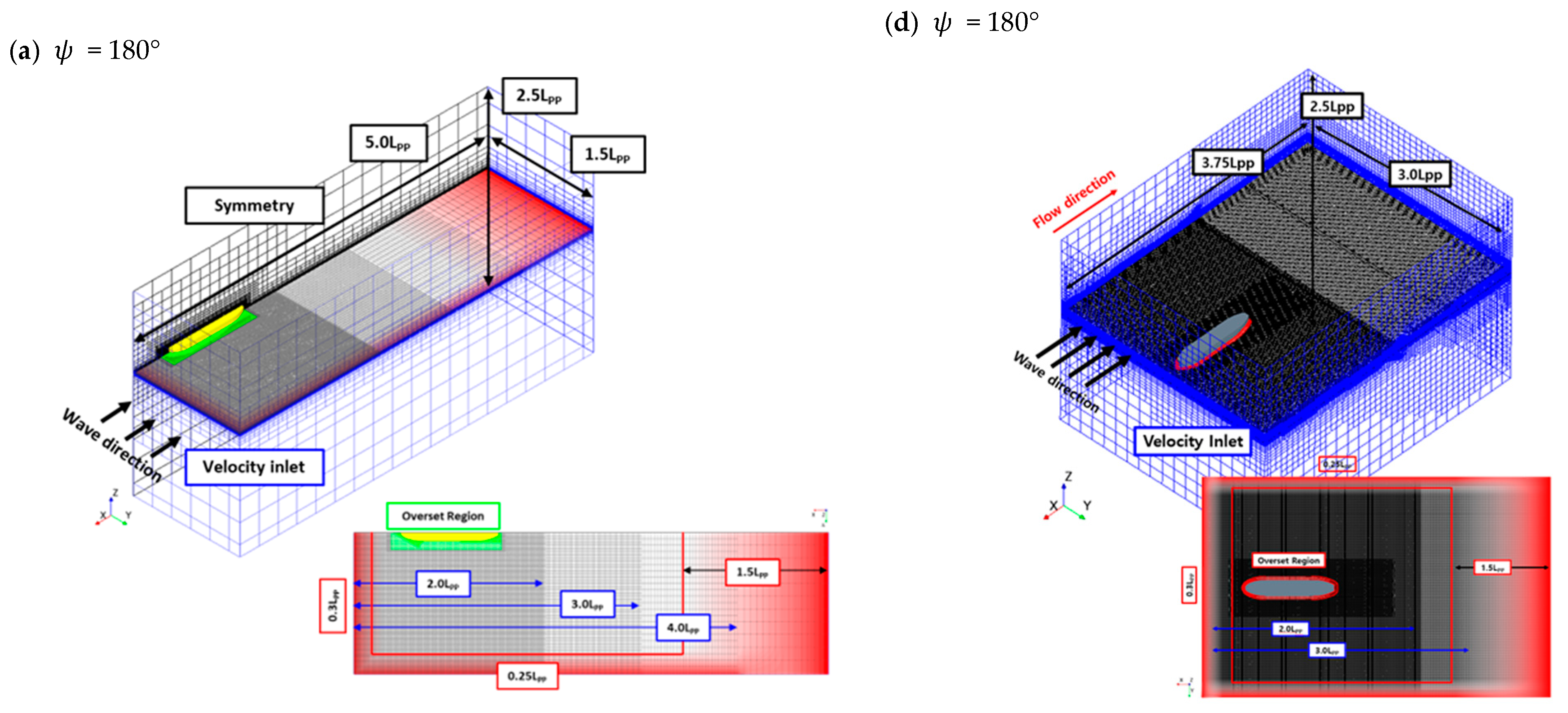
Three grid systems were used to evaluate the added resistance in oblique waves. First, in calm water and head sea ($\psi =180°$) conditions, calculations were performed using a captive model and soft-mooring system in half-breadth conditions, as shown in Figure 2a. The distance from the hull to the inflow boundary was 0.5$L_{PP}$, which is intended to minimize wave dissipation. A length of 3.5$L_{PP}$ was applied, including the grid damping area in the downstream area of the hull to prevent wave reflection. The length to the side and bottom boundary was 1.5$L_{PP}$, and the length to the top was 1$L_{PP}$.

To eliminate the effect of reflected waves in the numerical analysis domain, a wave-forcing condition was adopted at the inlet, outlet, and both sides, where the velocity inlet boundary conditions were applied. In the wave-forcing zone, we applied 0.3$L_{PP}$ to the inlet and both sides, and 1.5$L_{PP}$ to the outlet, to minimize the influence of waves reflected from the domain boundaries. For the boundary conditions, a velocity inlet condition was applied to the inlet, side (far from hull), outlet, and top and bottom. A symmetry condition was adopted on the side plane with the hull. A no-slip wall condition was applied to the hull.

In the case of the bow-quartering wave conditions ($\psi$ =150° and 120°), the full domain was applied with a symmetrical half-width domain, and a velocity inlet condition was applied as shown in Figure 2b,c. A trimmed mesh was used, which had the advantage in realizing the height of a wave. Approximately 2.6 million grid elements were used for the half domain, and approximately 6.2 million grid elements were used for the full domain. The numbers of grid elements in the overset region were 1.5 million and 3.1 million. To consider both the long- and short-wave regions, 120 grid elements per wavelength and 20 grid elements per wave height were applied at $\lambda /L_{PP}$ = 1.0 and $H/\lambda$ = 0.01.

The part marked with red is the wave-forcing area and was applied differently according to each boundary surface. The forcing boundary condition applies a theoretical wave to the boundary surface and minimizes the dissipation of the wave in the desired area by applying the transport equation in the input length. A forcing length of 0.3$L_{PP}$ was applied to the inlet, 0.25$L_{PP}$ applied to the side, and 1.5$L_{PP}$ applied to the outlet.

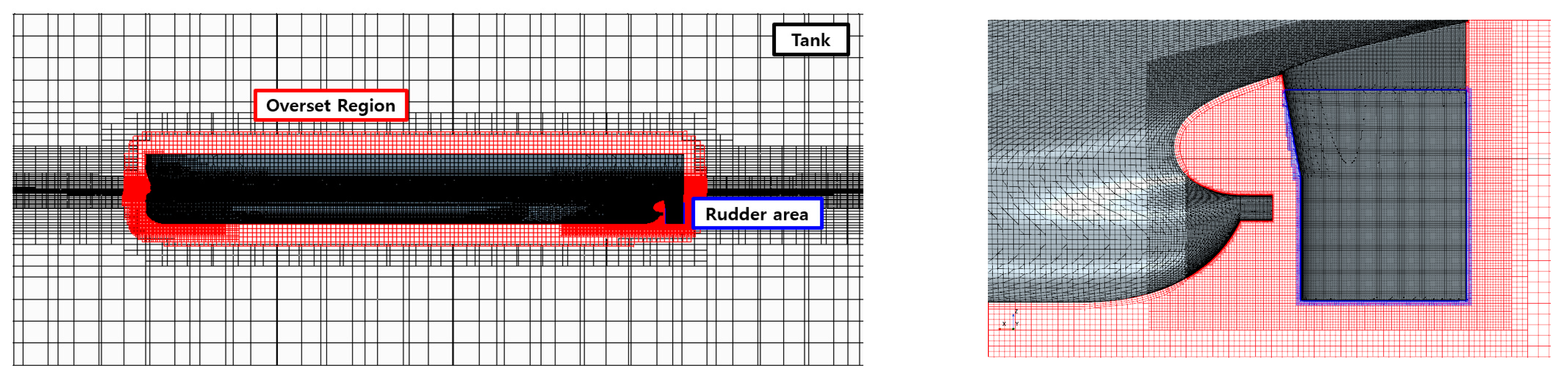
An adaptive mesh refinement (AMR) grid system was used for free-running calculations as shown in Figure 2d–f. The AMR grid can be adjusted so that the cell size becomes fine along the free surface based on the VOF, and the generated waves are accurately implemented without modifying the grid according to the wave conditions. Through a series of tests, the optimal parameters used for the AMR grid were determined as a transition width of 10 and a free-surface maximum refinement level of 4.

When using the AMR grid system, it is recommended to select an overset area that is a specific length away from the hull surface as shown in Figure 3, and the rudder area is applied as another overset grid system within the overset area to enable rotation. An oblique wave was considered as a method of rotating the ship for each heading angle in the same size domain. The domain was reduced by 0.75$L_{PP}$ in the longitudinal direction and 0.3$L_{PP}$ in the side direction compared to the fixed grid described above. Similarly, the wave-forcing area was set in the same way as in the fixed grid.

2.5. Soft Spring System

To apply the 6 DOFs without steering gear, the ship needs a means to regain non-restoring motions such as surge, sway, and yaw. In this study, a soft-mooring system was used, and a method of attaching two springs each to the bow and stern according to the height of the KG was chosen [13]. A spring can be implemented by defining a spring constant and location in STAR-CCM+. The force by the spring acts as an external force on the hull defined in DFBI. According to ITTC [24], when selecting the spring constant, it is recommended that the natural period of the spring be more than six times the wave generation period of the longest wave condition to be considered.

The spring’s natural period can be calculated by Equation (4):

$$T_s=2\pi \sqrt{\frac{m+m_a}{k_s} }$$

(4)

where $T_s$ is the natural period of the spring, $m$ is the mass of the ship, $m_a$ is the added mass of the ship, and $k_s$ is the spring constant [25]. In this study, a spring constant of 100 N/m with a sufficiently long natural period was selected. Figure 4 shows the soft spring system attached to the vessel and structure of springs in the numerical simulation.

2.6. Free-Running Model Test

A free-running model was adopted to implement 6 DOFs. For free running, the rudder and propeller rotation rate should be controlled to keep the same heading angle and self-propulsion state, respectively. A virtual disk was applied to mimic the propeller performance. The performance of the virtual disk of a KP458 propeller was verified through a POW test and showed similar results to the NMRI experimental results as shown in Figure 5 [26].

The target vessel of this study was an S-VLCC, but we tested whether free running can be implemented through STAR-CCM+ through a KVLCC2 hull. The type of rudder used was a horn-type rudder, as shown in Figure 6a. It was divided into a moving part (marked in red in Figure 6b) that can move to the port side and starboard side along the rudder axis, and a fixed part connected to the hull. The rotational speed of the rudder was limited to a maximum of 2.32 degrees/s on a full-scale basis, and the rudder can be rotated up to a maximum of 35 degrees.

PID control was used to adjust the aforementioned two variables. PID control was utilized in STAR-CCM+ by using the result for every iteration, which can be tracked using a field function, reported, and monitored. The PID gain value needed to be selected to adjust the propeller rotation rate and rudder angle. There are theoretical methods for selecting the PID gain value such as the Ziegler–Nichols method, but, in this study, the gain value was selected through a case study. As shown in

Table 3. Numerical analysis of test cases.

Case	${\mathit{K}}_{\mathit{P}}$	${\mathit{K}}_{\mathit{I}}$	${\mathit{K}}_{\mathit{D}}$	State
Propeller-V1	0.001	-	-	Long time to converge
Propeller-V2	0.05	-	-	Divergent
Propeller-V3	0.01	-	-	Long time to converge
Propeller-V4	0.01	0.05	-	Long time to converge
Propeller-V5	0.01	1		Converge high overshoot
Propeller-V6	0.01	1	1 × 10−5	Converge high overshoot
Propeller-V7	0.01	1	5 × 10−5	Converge
Rudder-V1	0.1	-	-	Divergent
Rudder-V2	0.01	-	-	Divergent
Rudder-V3	0.001	-	-	Divergent
Rudder-V4	0.001	0.1	-	Long time to converge
Rudder-V5	0.001	0.01	-	Long time to converge
Rudder-V6	0.001	0.1	0.1	Long time to converge
Rudder-V7	0.001	0.1	1.0	Long time to converge
Rudder-V8	0.02	0.1	1.0	Long time to converge
Rudder-V9	0.02	5.0	1.0	Fluctuation
Rudder-V10	0.02	5.0	5.0	Fluctuation
Rudder-V11	0.02	1.0	5.0	Convergence

, we tried to select a case with low vibration while converging quickly, which depends on the PID gain values. A total of seven propeller rotation rates were tested, from Propeller-V1 to V7, and a total of 11 cases were tested to adjust the rudder angle.

Figure 7a,b show the yaw angle and the rudder angle according to time, respectively, and the representative cases are plotted. As shown in Figure 7a, there is a difference in the yaw angle’s convergence time depending on the gain value. Through the case study, the most stable convergence case was selected and applied to subsequent calculations. The gain values applied to PID control were $K_P$ = 0.01, $K_I$ = 1.0, and $K_D$ = 5 × 10⁻⁵ for the propeller’s rotation speed, and $K_P$ = 0.02, $K_I$ = 1.0, and $K_D$ = 5.0 for the rudder angle.

2.7. Feasibility Test of Free Running Using KVLCC2

The feasibility of the added resistance computation in a wave was tested through the KVLCC2 at the design speed (Fr = 0.142) through the free-running state. The method for implementing the free-running technique was described in detail in Section 2.6. However, the propeller rotation speed should be adjusted to maintain the target ship speed during free running.

In this study, the point at which the average resistance and thrust are equal in waves was selected as the self-propulsion point. The resistance of the ship in the wave fluctuates with a large amplitude, as shown with the black solid line in Figure 8a. To maintain the self-propulsion point, the propeller rotation speed should oscillate, which is practically impossible. Therefore, by tracking the average values of resistance and thrust, the point where the two average values are equal was set as the self-propulsion point. The propeller rotation rate converges as shown in Figure 8b.

In the free-running state, the added resistance was estimated with Equation (5), which multiplies the difference between the average thrust value and the thrust in calm water by the thrust deduction factor.

$$\left(\overline{T_{Wave}}-T_{Calm}\right)\times \left(1-t\right)=R_{aw}$$

(5)

As a reference study, using the KCS hull, [27] Kim et al. (2021) compared the thrust deduction factor in calm water ($t_{Calm}$) and in wave conditions ($t_{Wave}$). Through CFD simulations, it was shown that the thrust deduction factor in waves tended to decrease. In particular, the decrease in the thrust deduction coefficient was the largest in the resonance region where the added resistance was the highest. Through this study, we compared the added resistance considering $t_{Wave}$.

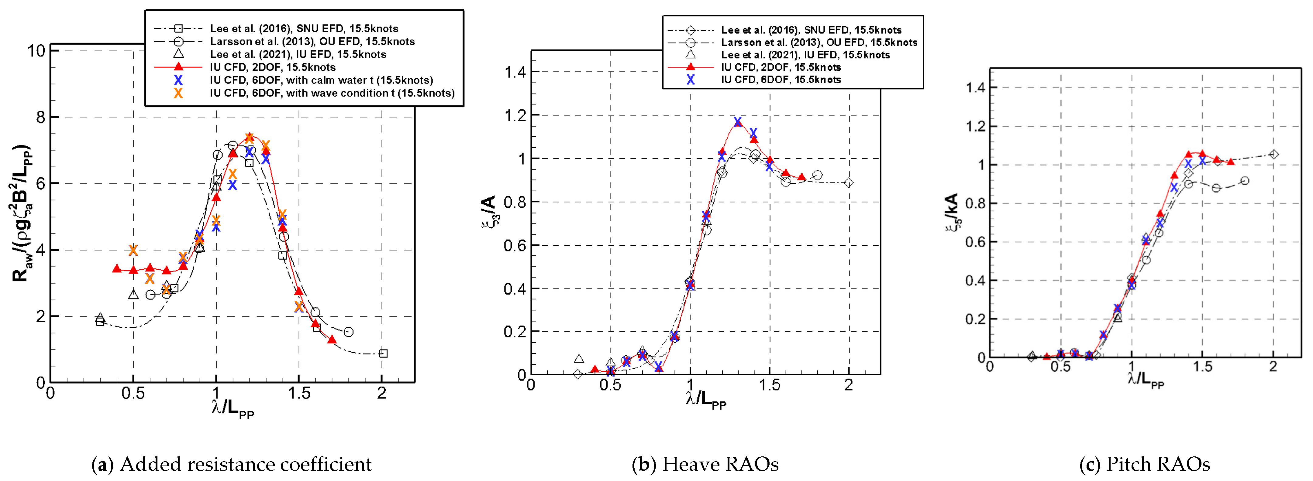
The added resistance coefficient in waves obtained through free running is shown in Figure 9, which was compared with the 2-DOF captive model results (with free heave and pitch). For the captive model, the results from Seoul National University (SNU) [28], Osaka University (OU) [29], and the Inha University Towing Tank (IUTT) [30] showed similar added resistance performance and motion RAOs. Therefore, the computation results are considered to follow the experimental results well. The added resistance coefficient in waves obtained in the free-running test showed similar results to the captive model, but, when $t_{Calm}$ was used, the measured added resistance coefficient was relatively low at the resonance frequency. To examine this, $t_{Wave}$ was compared as shown in Figure 10.

Lee et al. [30] compared the stern pressure in calm water and in a wave as a reason for the lower thrust deduction factor. They pointed out that the effect of the pressure change due to the suction of the propeller in the wave is reduced. They judged that the pressure of the stern part due to the movement of the hull during the wave changes regularly and is larger than the pressure changes due to the propeller.

Similarly, in this study, the change in the thrust deduction factor in free running was greatly reduced in the vicinity of the resonance frequency, where the propeller rotation rate is higher. The difference in the thrust deduction factor is not large compared to that in calm water at a short wavelength. As a result, it is reasonable to multiply the thrust difference by $t_{Wave}$ when calculating the added resistance coefficient in the wave with free-running conditions. In the case of using $t_{Calm}$, the added resistance near the resonant frequency of the ship was estimated to be relatively low.

2.8. Validation of Generated Regular Wave

A 3D wave test was performed to select CFD analysis conditions and parameters for the added resistance analysis. For the waves used for the 3D wave test, $H/\lambda =0.01$ and $\lambda /L_{PP}=1.0$ were applied to the S-VLCC with a scale ratio of 68. In the fixed grid system, 100 cells per wavelength and 20 cells per wave height were generated. The domain used in the computation is shown in Figure 11, and the area where the forcing conditions is applied is shown in Figure 11. The total number of grid elements was about 3 million, and the variables used in the wave test were reviewed by classifying the time discretization method and inner iterations as shown in

Table 4. Parametrically generated wave height verification.

Case		Fixed Grid				AMR
		D1I1	D2I1	D2I2	D1I2
Time step		$\mathsf{\Delta }T=T_{e=1.0}/400$
Time discretization		1st	2nd	2nd	1st	2nd
Inner iterations		8	8	10	10	10
Wave amplitude, error rate from theoretical value	at FP	−2.40%	−1.52%	−0.33%	−2.61%	−0.45%
	at Mid	−7.76%	−3.06%	−0.30%	−4.64%	−0.55%
	at AP	−12.1%	−5.98%	−2.03%	−8.73%	−2.30%

.

The generated waves, according to the parameters, were compared at the bow position (FP), the middle of the hull (Mid), and the stern position AP. When second-order time discretization was applied through D1I1 and D2I1, the wave dissipation was smaller than that of first-order discretization. Ten inner iterations showed better results compared with a theoretical wave than when eight iterations were applied. Therefore, in this study, D2I2 conditions were applied for the added resistance computations. In addition, the wave amplitude generated through the AMR method at the same domain size was compared, and it was confirmed that the reliability of the generated wave was sufficient when using the same conditions as D2I2.

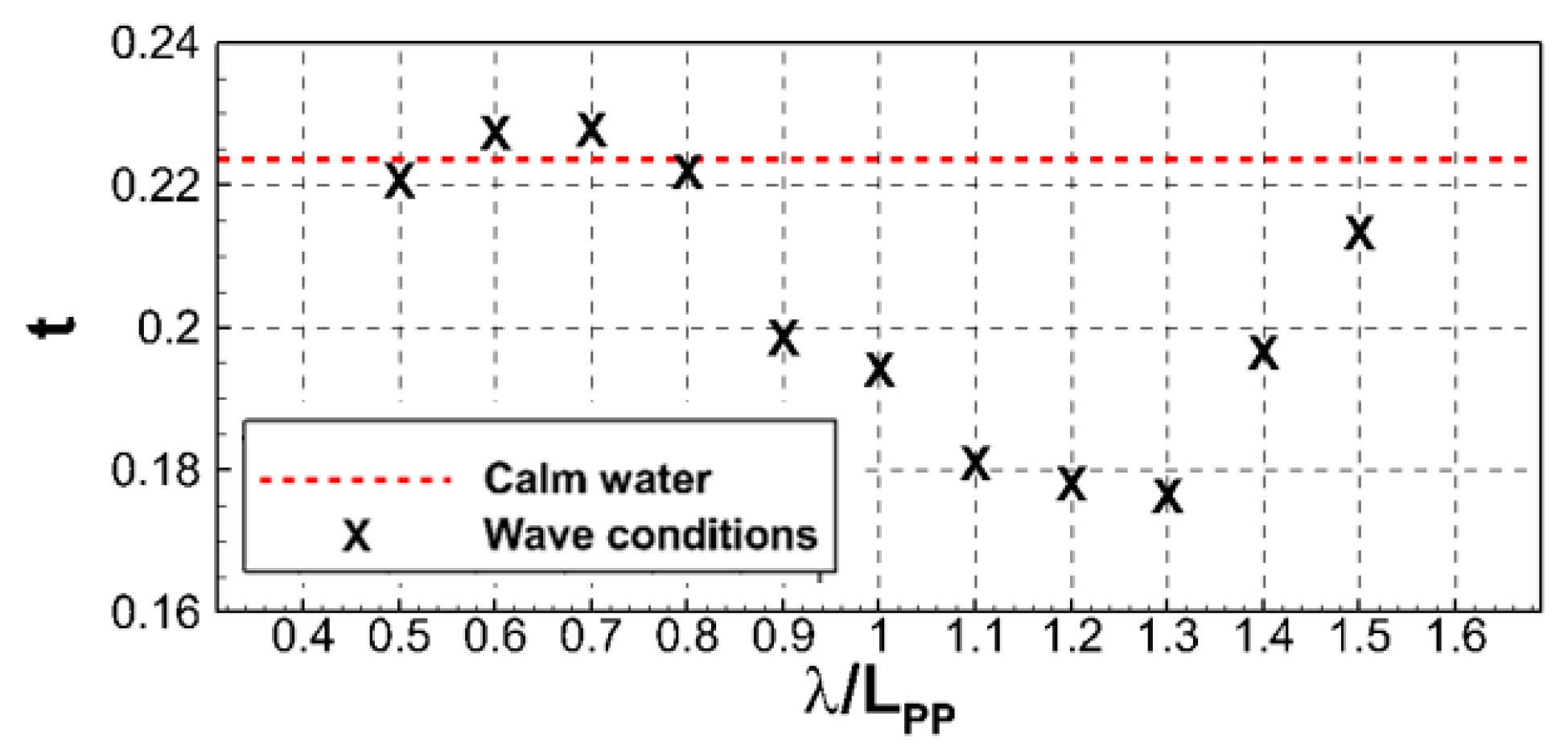
2.9. Convergence Test and Validation of S-VLCC Resistance Performance in Calm Water

A convergence test was conducted in calm water conditions to verify the calculations. Convergence was determined using the grid convergence index (GCI), which is based on the trend of outcomes from the refinement of the grid and time step [31]. The convergence parameters, time step, and grid density were evaluated in three stages.

Table 5. GCI of resistance coefficients and motion RAOs in regular wave ($Fr$ = 0.142).

Variables	Case No.	Number of Grid Elements	$\mathbf{\Delta }\mathit{t} \left(\mathit{s}\right)$	${\mathit{C}}_{\mathit{T}\mathit{M}}\times {10}^3$	GCI (%)	${\mathit{\zeta }}_3/\mathit{T}\times {10}^2$	GCI (%)	${\mathit{\zeta }}_5$ (deg)	GCI (%)
Time step	T1G2	2.4 million	0.04	4.615	2.17	3.886	4.07	0.143	0.87
	T2G2	2.4 million	0.02	4.463		3.902		0.145
	T3G2	2.4 million	0.01	4.387		3.918		0.146
Grid fineness	T2G1	0.5 million	0.01	4.984	0.000	3.853	0.004	0.143	0.524
	T2G2	1.5 million	0.01	4.773		3.918		0.145
	T2G3	2.4 million	0.01	4.386		3.918		0.146
	AMR-G1	1.1 million	0.01	4.705	0.024	3.844	0.000	0.142	0.021
	AMR-G2	1.4 million	0.01	4.768		3.832		0.144
	AMR-G3	1.6 million	0.01	4.975		3.970		0.151

shows the GCI of the resistance coefficients, sinkage, and trim.

First, computations were performed while changing the time step. The test was conducted by reducing the time step by 1/2 at 0.04 s, and the resistance, sinkage, and trim showed GCIs of 2.17, 4.07, and 0.87%, respectively. The computation results are sensitive to time step changes, and it was judged that the calculation sufficiently converged when the GCI value was less than 5%. The calculation was carried out based on the smallest time step of 0.01 s.

Next, a convergence test was conducted according to the density of the grid. The test was divided into a case using a fixed grid and a case using an AMR grid. Both grid systems showed a complete convergence of the calculations with a GCI index of less than 1%. In the finest condition, although the difference in the total number of grid elements of the two grids was about 0.8 million, the total computation time was similar. The AMR grid had a small number of grid elements, but it took more computation time until the grid converged, according to the free surface.

To validate the computation, the resistance performance in calm water was tested. The resistance coefficient, sinkage divided by the draft ($T$), and trim value were checked for differences from the experiment. As shown in

Table 6. Difference comparison with experiment.

		SNU EFD	INHA CFD, Fixed Grid	INHA CFD, AMR Grid
Scale ratio		100	68
ReM		2,489,775	4,433,761
Difference	$C_{TM}$ (Error rate)	-	4.96%	2.43%
	${\xi }_3/T\times {10}^2$	-	−1.06	−2.40
	${\xi }_5$ (deg)	-	0.044	0.032

, a total resistance coefficient with less than 5% difference from the experiment was obtained. There was a slight difference from the experiment in the sinkage and trim values. Although there was a difference in the exact value due to the scale difference from the experiment, it was judged that the CFD result was sufficient to express resistance and motion.

$$C_P=\frac{P-\left(\rho gh\right)}{1/2 V^2\rho }$$

(6)

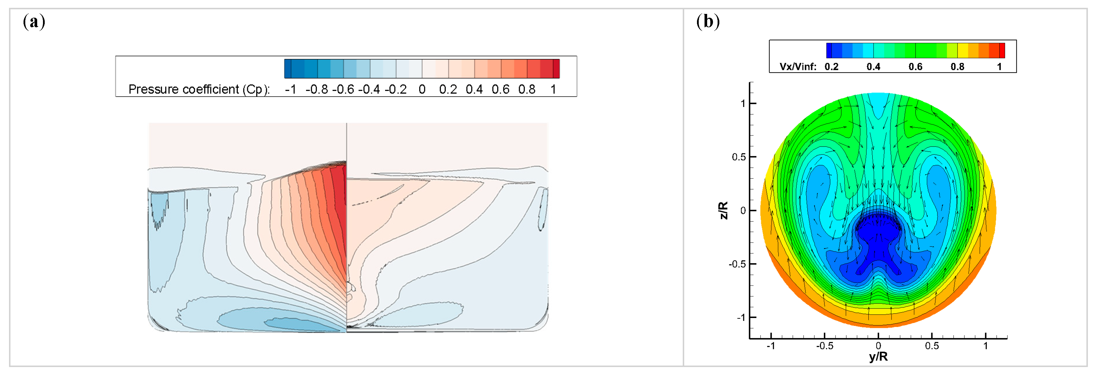
The dynamic pressure coefficient ($C_P$) and nominal wake in calm water are shown in Figure 12. The $C_P$ is calculated by Equation (6), where $P$ is a pressure, $\rho$ is a density, $h$ is a water depth from free surface, and $V$ is a velocity. High pressure was observed at the bow part, and, since there was no bulbous bow, the pressure tended to gradually decrease around the center of the hull. Pressure recovery was shown in the stern part and showed the pressure distribution of a general tanker. In the nominal wake distribution in the propeller plane, a distinct hook shape vortex was seen with a blunt stern shape, as shown in Figure 12b.

3. Results

3.1. Comparison of Added Resistance Performance of S-VLCC

The added resistance coefficient and the motion RAOs of the S-VLCC were studied at a speed of 15 knots in a head wave and bow-quartering wave ($\psi =150°, 120°)$. The numerical analysis results of this study were compared with two experiments (SNU and SSPA) and the Rankine panel method [11]. In the SNU experiment, a captive model test with 3 DOFs was applied, and the heave, pitch, and surge were free. The SSPA experiment was performed under free-running conditions.

The SNU model test was performed only in head wave conditions, and the SSPA model test was performed for all wave directions at 30° intervals from 180° to 0°. In this study, a 2-DOF (with free heave and pitch) computation was performed for head wave conditions. In the 150° bow-quartering wave condition, a computation of the captive model with 3 DOFs (with free heave, roll, and pitch) and 6 DOFs (soft mooring, free running) was conducted to compare the differences according to the DOFs. In the 120° bow-quartering wave condition, only the 6-DOF computations were performed.

Figure 13a–c show the added resistance coefficient under head and bow-quartering wave conditions. In the SNU model test, a general 2-DOF (heave and pitch) captive model test was performed to measure the added resistance and added resistance coefficient derived using the difference in resistance measured in a wave and calm water $\left(R_{AW}=R_{Wave}-R_{calm}\right)$. The SSPA test was a free-running test that measured the thrust in waves as $\left(R_{AW}=T_{Wave}-T_{Calm}\right)\left(1-t\right)$ and derived the added resistance coefficient in the wave using the thrust deduction factor ($t$). In general, the thrust deduction factor in calm water is used with the assumption that the difference in the thrust deduction factor should be small in wave conditions.

In head wave conditions, the added resistance coefficient showed a value similar to the results of the SNU model test and Rankine panel method. The tendency of the added resistance in the bow-quartering wave is similar to that in the SSPA model test results. On the other hand, similar to the KVLCC2 in Section 2.6, when using the thrust deduction factor in waves, the added resistance tended to appear relatively high. This is because the effect of propeller suction became stronger due to the increase in the number of rotations of the propeller due to the added resistance. This results in a difference in accuracy, but it is considered to be a small difference when considering the deviation of the experimental value itself.

Figure 13b shows the added resistance coefficient in the 150° bow-quartering wave conditions. The maximum value of the added resistance was similar to that at 180°; however, the position of the peak was shifted to a shorter wavelength. There was a minor difference in the results of the added resistance between the 3-DOF (with free heave, roll, and pitch) and 6-DOF computations when using the soft-mooring system. Moreover, the SSPA experiment showed a similar trend. However, in the case of free running, the added resistance was low around the resonant wavelength regardless of the thrust deduction factor used. The tendency appeared to be the same at 120°. Figure 13c shows the added resistance coefficient under the condition of a 120° bow-quartering wave.

In order to analyze the reason for the different added resistance in the case of soft mooring compared to the free-running result, the time-averaged sway and yaw motions of the soft-mooring case are shown in Figure 14 for each wavelength ratio. When using soft mooring, it was observed that the hull moved forward while maintaining a certain sway and yaw under the condition where the difference in the added resistance was large. This periodically recovered the non-restoring motion by the spring, but the ship advanced by a constant amount. The reason for having the largest motions under the condition of a wavelength ratio of 0.9 is that the energy of the wave is the highest because the wave height is the highest. On the other hand, in the case of free running, the average yaw motion does not happen because PID control is performed to maintain the yaw motion at 0. Moreover, a slight drift occurs in the sway direction during PID control, but the value is small and negligible.

With sway and yaw motions, the y-direction force and z-direction moment were compared. As shown in Figure 15, the force fluctuations that occurred in the time series appeared similar. However, when comparing the y-direction force and the z-moment coefficient obtained through the average value of the time series, a difference occurred as shown in Figure 16. This is because a restoring force was applied by the spring, and, in the case of free running, a relatively small y-force and z-moment were measured because propulsion occurs while maintaining a neutral angle using the rudder. The force and moment caused by the spring appeared larger at the heading angle of 120 degrees.

3.2. Comparison of Motion RAOs of S-VLCC according to Heading Angles

We compared the heave, pitch, and roll RAOs for each wave condition according to the heading angle. In Figure 13, the two model tests (SNU and SSPA) and the results of the Rankine panel method are compared with the captive model and the 6-DOF computation results of this study. First, as shown in Figure 17a–f, in the case of the heave and pitch RAOs, the motion response was similar regardless of the constraint conditions. As the heading angle increased, the encounter wave frequency decreased, and the resonant wavelength with the greatest motion RAO moved to a short wavelength. In the case of the pitch RAO, it tended to decrease as the heading angle increased, and, in the case of $\psi =120°$, it showed a hollow shape at $\lambda /L_{PP}=1.0$. As a result, the heave and pitch motions were judged to have little effect from the DOFs.

Figure 17g,h show the roll RAOs in bow-quartering wave conditions. The roll motion is greatly affected by the DOFs, and the difference is particularly large at the wavelength ratio corresponding to the roll natural frequency. At a heading angle of 150 degrees, the roll motion is the largest with 3 DOFs (with free heave, roll, and pitch), followed by soft mooring and free running. The heading angle of 120 degrees also had a large motion when soft mooring was used. With 3 DOFs, it is judged that the roll motion is large because the corresponding difference in the force acting on the hull is greater due to the restraints of the sway and yaw. In particular, the shape of a ship with a long slenderness ratio reacts sensitively to the roll motion and is greatly affected by external forces such as those from restraints in the DOFs or springs. In conclusion, the SSPA experiment and CFD results are most similar under the free-running test conditions.

3.3. Comparison of Flow Regime of S-VLCC at Stern according to Heading Angles

In order to compare the flow distribution around the hull according to the wave direction, streamlines passing around the hull were compared under the condition of $\lambda /L_{PP}=1.0$. The distribution of streamlines passing through $X/L_{PP}=0.03$ and $X/L_{PP}=0.1$ in the forward direction of the AP was compared, as shown in Figure 18 and Figure 19. Moreover, wall shear stress contours were shown on the hull surface. The corresponding streamlines and wall shear stress distributions are the results of time-series averaging.

First, as shown in Figure 18a–c, the flow passing the stern end is mainly affected by the flow rising up the hull. When the flow passes the center of the ship, the flow passing below rises along the skeg shape of the stern and then falls down, forming the flow on the upper part of the propeller surface. Figure 18d–f show the distribution of streamlines on the port side. In the oblique wave condition, the flow velocity is relatively high, and the frictional resistance at the top side is increased. In addition, the streamlines tended to spread widely to the bottom of the ship while flowing along the hull.

Conversely, Figure 18g–i show a distribution of streamlines on the starboard side. Unlike the port side, the flow speed slowed down, and the flow along the hull lasted for a long time, so, compared to the heading angle of 180 degrees, more streamlines were distributed above the hub. This is because the flow into the port side is blocked by the hull, and a low velocity section is formed above the hub.

In the same way, Figure 19 shows the streamline distribution that passes $X/L_{PP}=0.1$, which is the front part of the hull. The flow passing the bottom of the ship is predominant compared to $X/L_{PP}=0.03$. As shown in Figure 19a–c, the flow entering along the hull includes the flow rising from the ship bottom and the flow along the top of the skeg. Part of the flow past the bottom of the ship quickly passes the concave part of the stern and creates a swirling streamline. The rotational flow was asymmetrical in the oblique wave condition and appeared stronger on the port side facing the wave. The asymmetry is most evident in the 150-degree heading condition, and it is judged that the effect of the wave speed is relatively large in that condition.

When the port flow was compared using Figure 19d–f, the difference in streamline distribution was not large, but the shear stress at the bottom part was the largest at a heading angle of 120 degrees. Through this, it can be estimated that the flow velocity at the bottom part is fast under the most oblique wave condition. In Figure 19g–i, the flow velocity at the bottom of the ship in bow-quartering seas is faster on the starboard side compared to the bow wave condition. The streamlines near the hull are similar, and it is judged that the rotational strength was weakened due to the increase in flow speed, as shown in Figure 19a–c. To evaluate the trends of the previously compared flows with quantitative values, nominal wakes for each condition are compared in

Table 7. Comparison of nominal wake fraction, effective wake fraction, and propeller rotation rate.

Wave Condition	$1-{\mathit{w}}_{\mathit{n}}$	$1-{\mathit{w}}_{\mathit{t}}$	n (RPS)
Calm water	0.541	0.572	12.87
$\lambda /L_{PP}=1.0, \psi =180°$	0.546	0.625	14.55
$\lambda /L_{PP}=1.0, \psi =150°$	0.567	0.595	14.95
$\lambda /L_{PP}=1.0, \psi =120°$	0.560	0.602	14.05

. Moreover, Figure 20 shows the distribution of the averaged axial velocity entering the propeller plane in wave conditions compared to calm water conditions.

When comparing the nominal wake coefficient values, the flow rate increases in wave conditions compared to the calm water condition. In terms of the effective wake coefficients, different trends were shown for each condition. It is thought that the added resistance increases the number of rotations of the propeller in the wave, and, as a result, a difference in effective wake occurs due to the influence of the nominal velocity and the interaction velocity. In the wave condition, at the heading angle of 150 degrees, the propeller’s rotation rate was highest, and the effective wake fraction value was lowest (the heading angle of 180 degrees showed the highest value). Therefore, it is difficult to find the trend of the effective wave direction, because the effect of the inflow velocity and the increase in the propeller rotation speed are complex.

In the wake distribution in Figure 20, it is shown that the low-speed section of the hook shape is reduced in the wave conditions. The overall flow speed increased, and an asymmetrical nominal wake was observed in the bow-quartering sea condition. The low-speed section at the top of the shaft tended to be biased to the left, and the bias was greater at the heading angle of 150 degrees.

The wake distribution for each encounter period ($T_e)$ among waves is compared in Figure 21. The encounter period was divided into four parts with time ($t$), and the point where the wave crest crossed the bow was considered as 0. Figure 21a–d show a bow sea condition in which the wake swings up and down. At $t/T_e=1/4$, where the crest of the wave comes to the middle of the hull, the flow tended to rise upward, which seems to be caused by the rise of the stern. At this time, the high-speed region is widely distributed, and the inflow velocity increases. Conversely, the flow slowed down the most at $t/T_e=3/4$, where the stern descended.

Under the bow-quartering wave condition, the flow tended to come and go in a tilted line because the hull moved in an oblique direction. In Figure 21e–h, the wake change at $\psi =150°$ showed a wide high-speed region when the wave crest passed the bow, unlike at $\psi =180°$. Moreover, through the vector distribution, the overall flow velocity was fast, and a strong vortex occurred at $t/T_e=3/4$. Even during one cycle, the direction and speed of the flow changed drastically and asymmetrically.

In Figure 21i–l, the trend is the same under the heading angle condition of 120 degrees, and the bias of the flow was less than that at 150 degrees. It is judged that the movement of the hull is reduced when the wave direction is relatively large, so the flow change is also reduced. Due to the following wake changes, it is difficult to estimate the effective wake fraction value in oblique wave conditions. In addition, since the wake in calm water is taken into consideration when designing the propeller, it causes a change in the propeller efficiency in waves.

4. Conclusions

This study analyzed the added resistance performance of ships in various wave conditions according to constraint conditions through CFD. The target ship’s added resistance coefficient and motion RAOs were compared using a 2-DOF captive model (with free heave and pitch) and a 3-DOF model (with free heave, roll, and pitch). Moreover, a soft spring system and free-running model were applied to simulate 6-DOF conditions. A 6-DOF soft-mooring system was simulated through spring coupling in the DFBI body.

• When calculating the added resistance through the free-running model, it was verified through two hulls that the added resistance showed a similar trend compared to the experiment in head sea conditions. On the other hand, both hulls showed a difference in the value of added resistance according to the thrust deduction factor used. It was assumed that the thrust deduction in waves was similar to that of calm water, but, under the conditions of high wave height and high added resistance, a difference in the thrust deduction compared to calm water can be shown due to the increase in the number of propeller revolutions. The difference was relatively insignificant under the condition of a wave steepness of 0.01, but, when using a higher wave steepness, it is necessary to consider the change of the thrust deduction factor in wave conditions.
• In terms of the added resistance coefficient, the difference in estimated values was not large according to the DOFs. In a bow-quartering sea, as the heading angle of the ship decreased, the peak wavelength of the added resistance moved to a shorter wavelength, and the magnitude decreased. On the other hand, the added resistance in the free-running condition was lower than with the soft-mooring system. To analyze the cause of the difference, the y-force and z-moment on the hull were compared. The amplitude of fluctuations according to the time series was similar, but the time-averaged y-force and z-moment occurred when soft mooring was used. In addition, the yaw and sway occurred along with force, which is considered to be one of the causes of increased added resistance.
• The influence of the heave and pitch motions according to the DOFs (3 DOF and 6 DOF) with a 150-degree heading angle was insignificant. However, in the case of the roll motion, the 3-DOF (with free heave, roll, and pitch) model overestimated the roll motion more than the 6-DOF model. A corresponding trend was also found between the soft-mooring system and free running at the heading angle of 120 degrees. The roll motion is sensitive to the DOFs and depend on the case where the sway and yaw are constrained or interfered with by a spring. Therefore, to accurately estimate the motion response in the oblique waves, a computation should consider the 6-DOF motion of the ship.
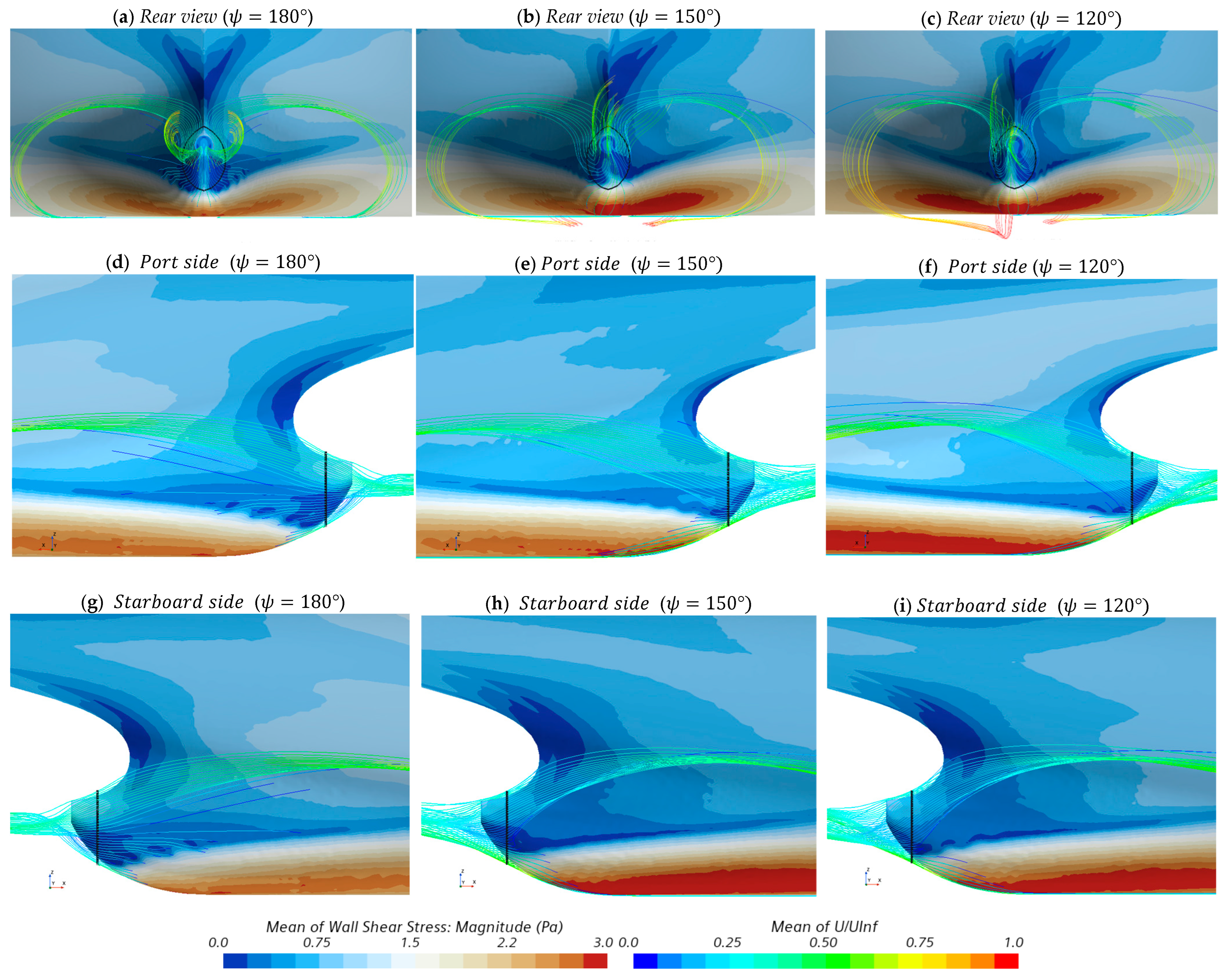
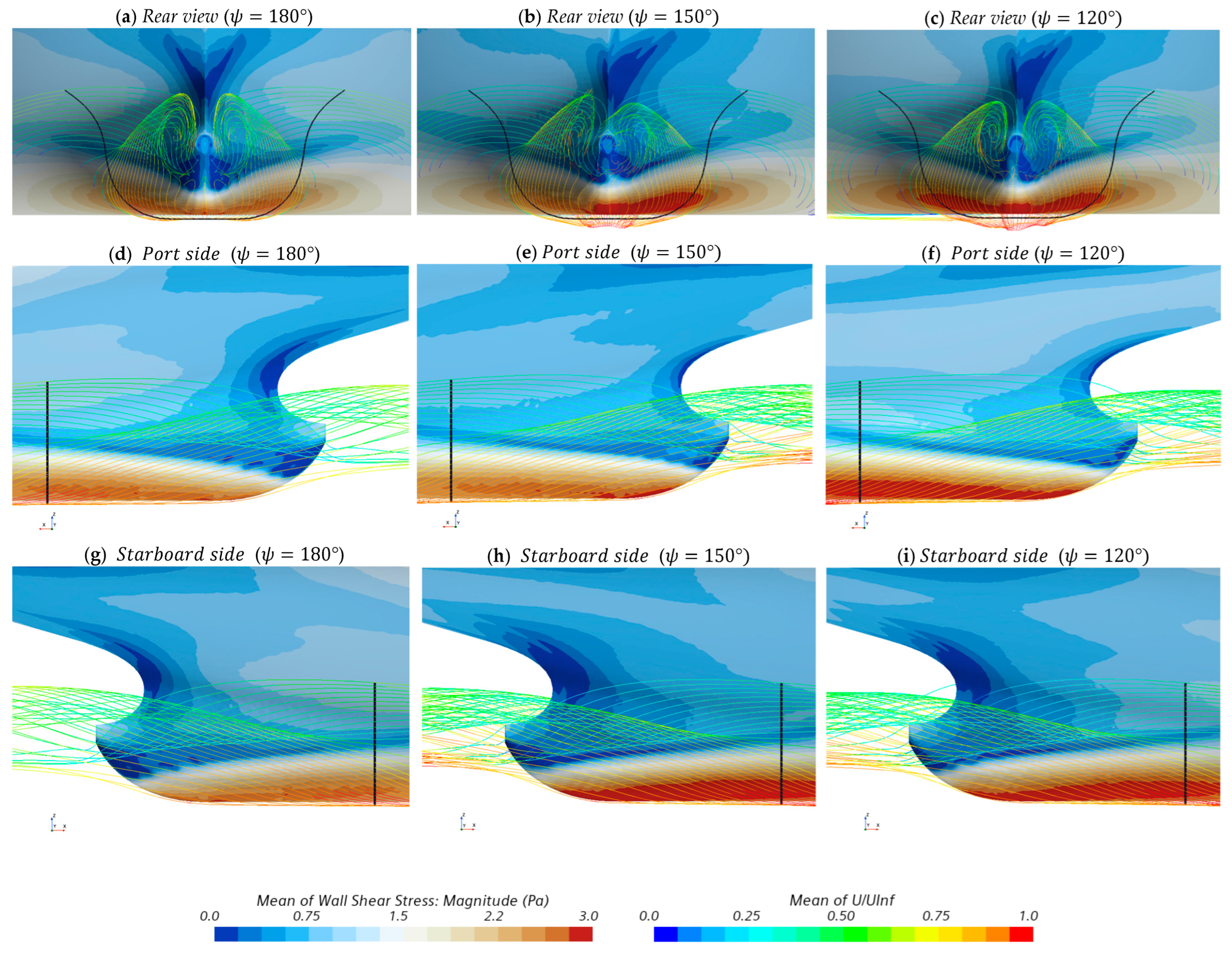
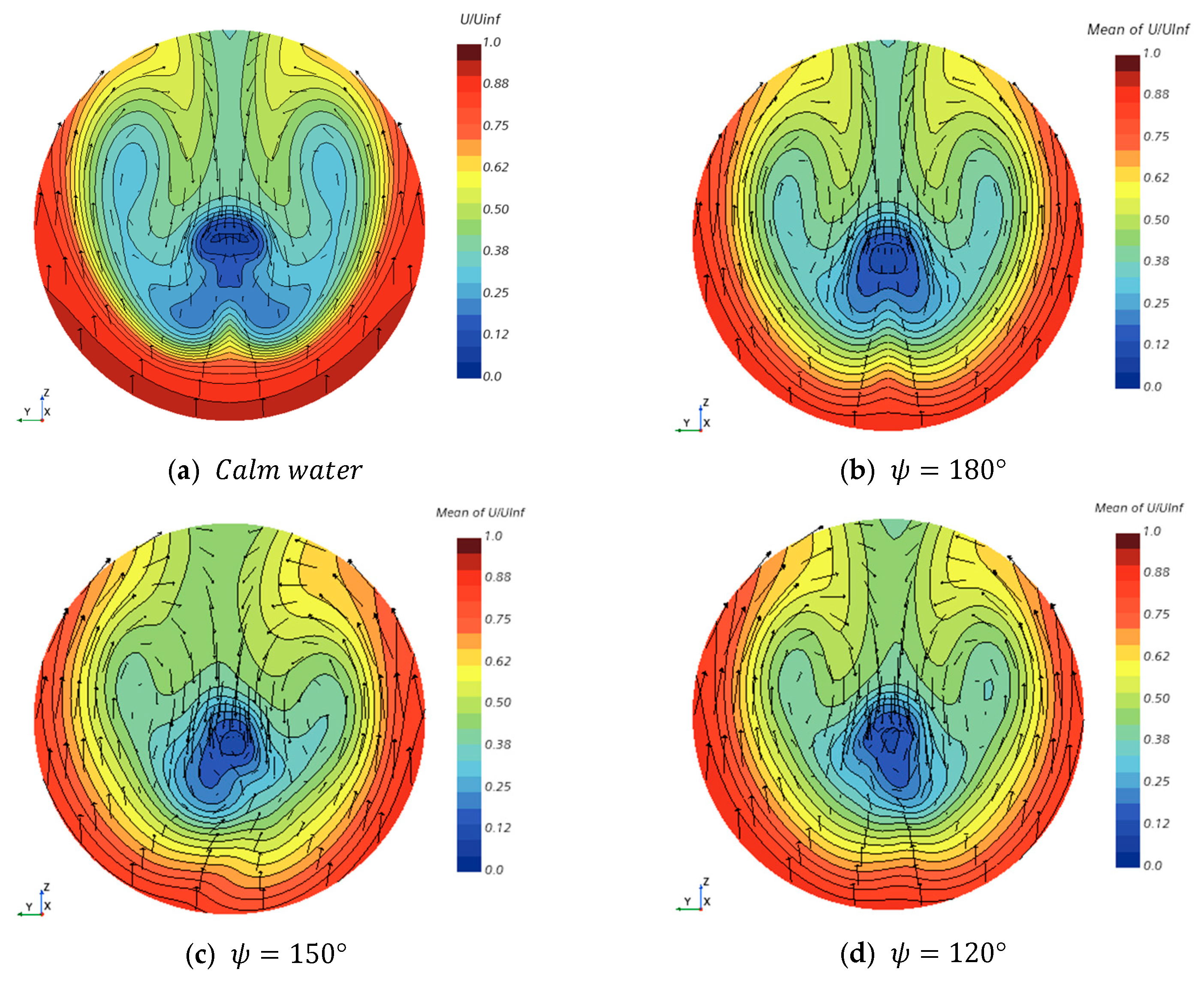
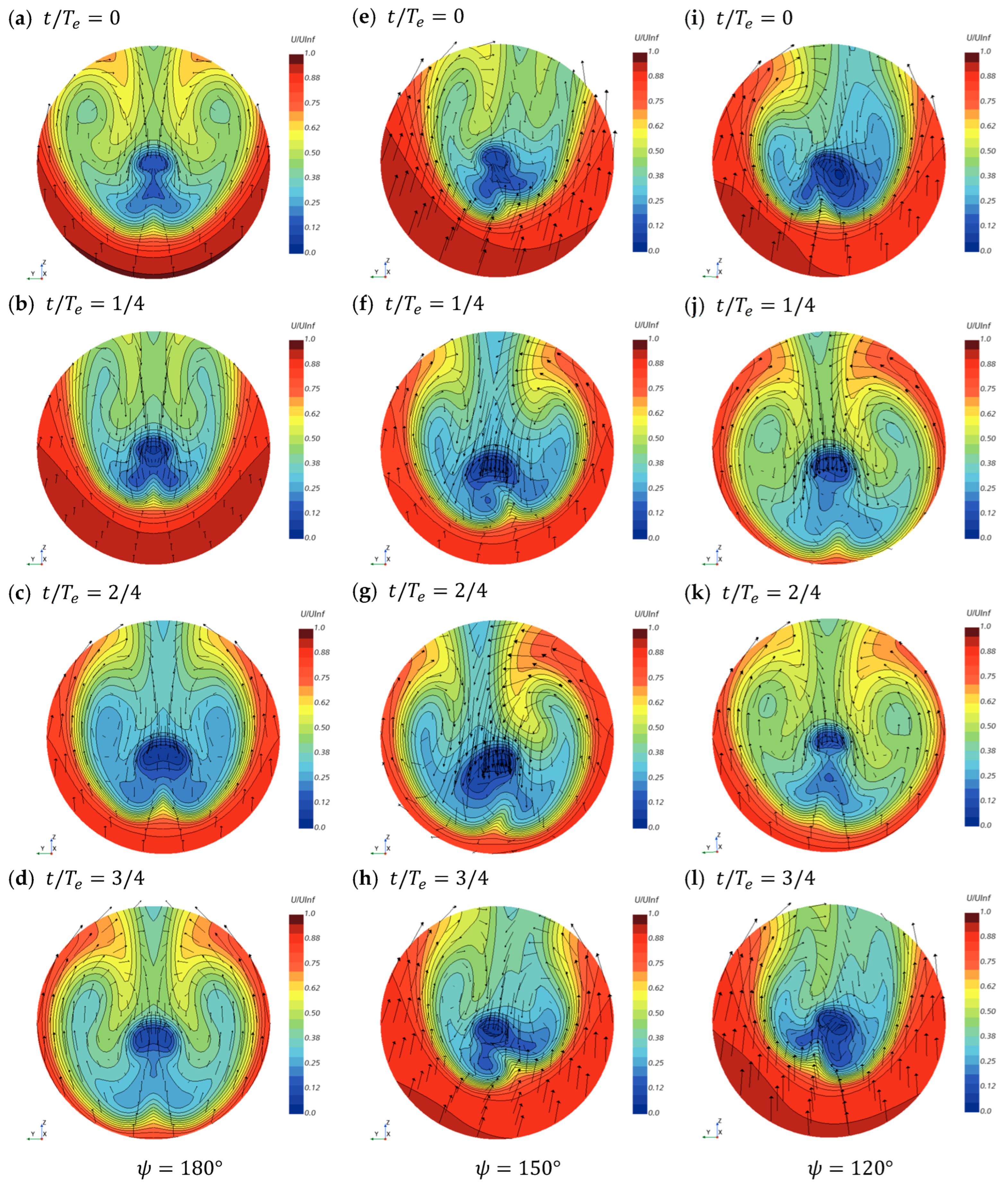
• When using the soft-mooring system, it is possible to observe the flow around the hull that occurs along the wave direction. In this study, the streamlines and nominal wake for each heading angle were compared under the condition of a wavelength ratio of 0.1. The streamline passing $X/L_{PP}=0.03$ from the AP position passes the upper part of the wake plane and flows past the hollow of the stern. In the bow-quartering sea condition, the distribution of streamlines on the left and right changes asymmetrically, and the flow on the port side becomes relatively fast, bringing the streamline distribution closer to the keel line. On the other hand, the streamline passing $X/L_{PP}=0.1$ was generally distributed in the wake plane, and the flow past the lower part of the hull was predominant. In particular, it was estimated that the flow was the fastest due to the high shear stress at the heading angle of 120 degrees.
• The mean nominal wake flow velocity increased in oblique wave conditions. The asymmetry of the nominal wake was greatest at a heading angle of 150 degrees. The effective wake was difficult to estimate due to the combined effects of the faster axial velocity and the increase in the propeller’s rotational speed. In addition, when comparing the nominal wake distribution for each wave cycle, the wake change for each encounter wave period was large. The main cause of the wake change was the movement of the ship, and the change was most rapid at the heading angle of 150 degrees, where the movement was the largest.

Through this study, it was confirmed that the 6-DOF implementation method used in the experiment can be reproduced through CFD. Through the simulations, there are differences in the added resistance performance and motion response depending on the constraint conditions and test method. In addition, it was shown that the flow distribution around the hull can change significantly in an oblique wave. For future study, the plan is to observe the added resistance performance using a captive model, a soft-mooring system, and free-running conditions for the same vessel. The flow distribution will be compared under more wave conditions, and we will observe changes in the self-propulsion factors and the number of propeller revolutions during free running. Finally, an irregular wave condition will also be tested.