Article

Water Properties and Diffusive Convection in the Canada Basin

1
Hubei Key Laboratory of Resources and Eco-Environment Geology, Hubei Geological Bureau, Wuhan 430034, China
2
Geophysical Exploration Brigade of Hubei Geological Bureau, Wuhan 430056, China
3
State Key Laboratory of Tropical Oceanography, South China Sea Institute of Oceanology, Chinese Academy of Sciences, Guangzhou 510301, China
4
University of Chinese Academy of Sciences, Beijing 100049, China
5
Sanya Institute of Ocean Eco-Environmental Engineering, Sanya 572025, China
6
School of Industrial Design and Ceramic Art, Foshan University, Foshan 528000, China
7
College of Environment and Engineering, Hubei Land Resources Vocational College, Wuhan 430090, China
*
Authors to whom correspondence should be addressed.
J. Mar. Sci. Eng. 2024, 12(2), 290; https://doi.org/10.3390/jmse12020290
Submission received: 14 December 2023 / Revised: 29 January 2024 / Accepted: 2 February 2024 / Published: 5 February 2024
(This article belongs to the Special Issue Investigating the Air-Sea Interaction Processes)

Abstract

:
The aim of this study is to better understand diffusive convection (DC) and its role in the upper ocean dynamic environment and sea ice melting in the Canada Basin. Based on a moored dataset with 6737 profiles collected from August 2003 to August 2011 in the upper layer of the Canada Basin, DC between the warm and salty Atlantic Water (AW) and the colder and less salty Lower Halocline Water (LHW) were investigated. The moorings were designated at four stations: A, B, C, and D, located at the southwestern, southeastern, northeastern, and northwestern parts of the basin, respectively. During the observation period, the temperature, salinity, and depth of the AW and LHW exhibited unique temporal variations. The temperature and salinity of the AW varied among stations, with a decreasing trend from northwest to southeast, consistent with the propagation path of the AW in the Canada Basin. The temperature and salinity of the LHW were similar at all stations. The AW and LHW cores were located between depths of 320–500 m and 160–300 m, respectively, and both gradually deepened over time. Distinct DC staircase structures were observed between the AW and LHW, more pronounced at stations C and D than at stations A and B, which is speculated to be related to eddies at stations A and B during the observation period. The vertical heat fluxes through the DC staircase layer at stations C and D (FHc_C and FHc_D) were estimated using an empirical formula. FHc_C ranged from 0.05 to 0.94 W/m2, and FHc_D ranged from 0.05 to 0.6 W/m2, with the maximum probability value for both at approximately 0.2 W/m2. The effective diffusivities at these two stations (KT_C and KT_D) are similar, ranging from 2 × 10⁻⁶ to 3 × 10⁻⁵ m2/s, with the highest probability occurring at 6 × 10⁻⁶ m2/s. Both the probability density function of the heat flux and the effective diffusivity skewed towards larger values and obey a lognormal distribution, indicating turbulence intermittency of the DC staircase in the Canada Basin. These finding offers new insights into the heat transport and turbulence in the DC staircase, and then bring a deeper understanding of sea ice melting in the Canada Basin.

1. Introduction

In the ocean, there is a significant difference in the diffusion of heat ( κ T 10 7 m 2 / s ) and salt ( κ S 10 9 m 2 / s ) transport at the molecular scale, with thermal diffusivity being approximately 100 times that of salt diffusivity. Temperature and salinity have opposite effects on the density gradient of seawater, and possess the conditions for the occurrence of the double diffusion phenomenon [1]. Double diffusion includes two types: salt finger and diffusion convection (DC). When high-temperature and high-salinity water is above low-temperature and low-salinity water, salt finger is generated, which mostly occurs in the pycnocline of tropical and subtropical seas. When low-temperature and low-salinity water is above high-temperature and high-salinity water, it is easy to generate DC, which mostly occurs in the Arctic Ocean and other polar seas [2,3,4]. The main feature of DC is that its temperature and salinity profiles have a staircase structure, which is composed of consecutive thick mixed layers where the temperature and salinity are uniform and thin interfaces with a large gradient.
Atlantic Water (AW) has the characteristics of high temperature and high salinity (with a potential temperature above 0 °C and a salinity of about 35–36 psu), entering the Arctic Ocean through the Fram Strait and Barents Sea branches, entering the Canada Basin through the Eurasian Basin [5], and widely distributed at depth ranging from 300 to 550 m. The Fram Strait branch flows through the northern part of the Chukchi Plateau into the Canada Basin, with its salinity ranging from 34.80 to 34.86 psu at the depth where the maximum potential temperature θmax is found [5]. In contrast, the Barents Sea branches, which have lower temperatures and higher salinity, enter the central Arctic Ocean through the Kara Sea and Santa Anna Trough. These branches then flow eastward along the Eurasian continental slope and are distributed in deeper locations [5]. Once these high-temperature waters enter the Canada Basin, they follow a cyclonic path within the basin. If all the heat carried by these waters is transferred to the sea surface, it has the potential to melt all the sea ice within a few years [5,6]. However, the strong stratification between surface and subsurface water layers limits the upward transport of heat [7].
Above the high temperature and high salinity waters of the North Atlantic, there is Low Halocline Water (LHW) with low temperatures and low salinity. There are two types of LHW: oxygen-rich LHW and hypoxic LHW. The oxygen-rich LHW originates from the winter mixed layer of the Nansen Basin, enters the Makarov Basin through the Lomonosov Ridge, and enters the Canada Basin between the Alpha Ridge and Mendeleyev Ridge [8]. It is mainly distributed in the northern part of the Canada Basin. Hypoxic LHW originates from the Chukchi shelf region and is formed through cross-density mixing between Pacific winter water and upper Atlantic water. It is mainly distributed in the southern part of the Canada Basin and is widely distributed at a depth ranging from 150 to 300 m.
The DC phenomenon between LHW and AW exhibits a staircase structure in both its temperature and salinity profiles [9]. The DC staircases exist in relatively quiescent region [10]. It is energetically quiescent in the Arctic Ocean’s central basins [11]. Ménesguen et al. reported that the DC staircases gradually vanished in the Canada Basin [12]. Mclaughlin et al. proposed that the thermohaline intrusions in AW show signs of dissipation near the Northwind Ridge, which indicated that, as temperature gradients decrease, they will disappear from the Canada Basin [13]. Bebieva et al. suggested that the rundown of the thermohaline intrusions may form staircases [14]. The study by Ainslie provided insight into the formation and destruction of DC staircases in Arctic Ocean [15]. The AW has been warming in the Canada Basin based on the observational data from the Larsen-93 expedition in 1993 [16]. It is believed that the DC staircase is a necessary pathway for AW to transport heat and salt upwards, and it plays a crucial role in the heat flux transport within the Arctic Ocean [13,14,17,18,19]. Ruddick and Gargett suggested that the small-scale DC staircase structure is influenced by the large-scale circulation caused by the vertical temperature and salinity gradients, as well as the shear caused by large-scale lateral disturbances [20]. The transport flux of DC has a significant impact on the circulation and large-scale ocean characteristics. Previous laboratory experiments have shown that the strength of stratification and bottom heating of water bodies can affect the melting rate of sea ice on the surface [6]. This indicates that the stratification strength and variability of AW in the Canada Basin will have a significant impact on the melting of sea ice. The stratification strength in the Canada Basin is primarily influenced by the vertical interaction of water masses. AW and LHW are the main water masses in the upper layer of the Canada Basin, and any changes in these water masses will profoundly affect the hydrological environment of the Canada Basin.
Several studies have estimated the heat flux transmitted upwards by the AW through the DC staircase in different regions. Zhao et al. used observational data from the Arctic scientific expedition of China in 2008 to analyze the characteristics and spatiotemporal distribution differences in the DC staircase in the Canada Basin, and estimated the AW vertical heat flux caused by DC to be 0.05–0.22 W/m2 [21]. Padman and Dillon estimated that the heat flux transmitted upwards by AW through the DC staircase in the Canada Basin to be 0.02~0.10 W/m2 based on observed micro-structural [22,23]. Polyakov et al. estimated that the heat flux transmitted upwards by AW through DC staircase in the central part of the Laptev Sea slope was 2–8 W/m2, based on data profiles from 2007 to 2008 [17]. Song et al. analyzed heat flux of AW transported upwards through DC staircase in the Arctic Ocean using Ice-Tethered Profiler (ITP) data, which was less than 0.5 W/m2 [24]. Qu et al. analyzed the interaction between the DC staircase and AW/LHW based on mooring data from 2005 to 2011 in the Canada Basin [9]. They estimated the heat flux transmitted upwards by AW through the DC staircase to be 0.05–0.60 W/m2, and discussed the vertical distribution of heat flux and the eddy diffusion coefficient. With the mooring data from the Canada Basin, Lique et al. estimated the heat flux to be in the range of 0.1~0.2 W/m2 on average [18]. Based on Ice-Tethered Profilers data, Bebieva and Timmermans found that the heat flux was in the range of 0.2~0.3 W/m2 [14].
While previous studies have shed light on the significance of water masses and the DC staircase in the Canada Basin, mainly focusing on their structural characteristics and interactions, there remains a need for a more comprehensive understanding of the spatiotemporal changes in the AW and LHW, as well as in the patterns of DC over time and space. This research seeks to address this gap by delving deeper into the spatiotemporal characteristics of water masses and the DC staircase within the Canada Basin. By investigating the spatiotemporal variations of the AW and LHW, as well as the DC staircase, and estimating vertical heat flux across DC staircase, diapycnal mixing of DC staircase, this study can enhance our understanding of the Canada Basin’s physical and ecological environments.
In this paper, we first compare the AW and LHW at four mooring stations within the Canada Basin, in terms of their variations of potential temperature, salinity, and depth. We then compare the persistence of the DC staircase at these four stations. Finally, we estimate the heat flux transferred upwards by AW through the DC staircase at the stations C and D, as well as the effective vertical diffusivity resulting from the presence of DC.

2. Observational Data and Methods

2.1. Observational Data

In this work, the data used were collected from four moorings deployed within the Canada Basin as part of the “Beaufort Gyre Freshwater Experience” project by the Woods Hole Oceanographic Institution from August 2003 to August 2013. The data were downloaded from https://www2.whoi.edu/site/beaufortgyre/data/mooring-data/ (accessed on 25 January 2014). The detailed process of pre-processing MMP data can be found in the technical report “ BGFE 2003–2004 MMP EMCTD and ACM Data Processing Procedures” by Krishfield R et al. (unpublished, available for download at http://www.whoi.edu/page.do?pid=66566 (accessed on 23 April 2013)). As shown in Figure 1, these moorings, labeled as A, B, C, and D, were equipped with McLane Moored Profile (MMP) instruments. The instrument configuration and data details have been described in a previous study by Qu et al. [9]. The sampling time, location, and number of profiles of the MMP are shown in Table 1. A total of 6737 MMP profiles were collected between 2003 and 2011. After preprocessing, the vertical resolution of the data was 2 m, with a measurement depth range of 60–2000 m. The sampling time intervals between profiles were 6 h and 48 h, depending on the diving and floating schedule of the MMP (MMP diving and floating time intervals were 6 h, and the time interval between floating and next diving was 48 h).

2.2. Typical Hydrographic Profile

A typical MMP profile is shown in Figure 2, which was recorded at the Station D at 6 am UTC (Universal Time Coordinated) on 19 November 2006. Based on the previous studies [9,17,25,26], the core of the AW is defined at the depth of the maximum subsurface potential temperature θ, and the core of the LHW is defined at the salinity S = 34.1 (Figure 2a). Figure 2b shows the θ and S profiles with depth. The warm and salty AW lies beneath the cold and fresh LHW. The vertical distributions of θ and S reveal that both of them increase with depth, which is conducive to the formation of DC staircase. Figure 2c shows the local enlargement of the θ and S profiles between the LHW and AW. It is found that the DC staircase, consisting of continuous steps, appears between the depth of 300 m and 400 m. Each step contains a thick homogeneous mixed layer and a relatively thin interface layer with a large-gradient interface. Half of the upper and lower interfaces, along with the mixed layer, form a convective cell, which is considered to have similar structural characteristics to the Rayleigh–Bérnard convection [9,27,28,29,30].
The stability of the DC staircase is generally characterized by the density ratio Rρ and the buoyancy frequency N, which are important parameters in understanding the physical properties of the staircase structure [3]. The density ratio Rρw and the buoyancy frequency Nw between AW and LHW are defined by following the approach in Bourgain et al. [31]
R ρ w   =   β S A W S L H W α θ A W θ L H W
N W   =   g α ( θ A W θ L H W ) β ( S A W S L H W ) Z A W Z L H W .
where the subscripts AW and LHW characterize the physical quantities corresponding to AW and LHW water masses, respectively. θ is potential temperature, S is salinity, Z is depth, g is the acceleration due to gravity, α is the coefficient of thermal expansion, β is the coefficient of haline contraction.

2.3. Identification of the DC Staircase

The thin diffusion interfaces of DC are characterized by large salinity variance, while the consecutive thick mixed layers are characterized by almost uniform salinity. The salinity variance in the mixed layer is about 0.0027 and the salinity variance the in diffusion interface is about 0.02 due to empirical observations from the vertical profiles of salinity. Figure 3 shows the salinity data measured at the four stations, A–D, during the observation period from 2003 to 2011. Each black dot in Figure 3 represents a salinity value at one depth. It is well known that the mixed layer is much thicker than the diffusion interface; it also means that the salinity values in the mixed layer are more concentrated and roughly kept continuous and constant. It can be seen that the concentrations of the black dots within the mixed layer and the diffusion interface are significantly different. The black dots are densely distributed within the mixed layers, forming black strip-like structures. This is also consistent with the characteristics of almost uniform salinity within the mixed layer. From Figure 3 we can see that the DC staircases were present at these four stations during the observation period, and the staircases at stations C and D were more prominent than those at stations A and B.
To analyze the temporal variation in each step, it is necessary to identify all the steps from the staircase at each station. Due to the fact that the diffusion coefficient of temperature (κT ≈ 10−7 m2/s) is much larger than the diffusion coefficient of salinity (κS ≈ 10−9 m2/s), within the mixed layer the salinity fluctuation is much smaller than the temperature fluctuation [9], thus we used the fixed-salinity method to identify the steps from the staircase. A detailed introduction to this method can be found in the study by Lu et al. [32], and here we only provide a brief description. Probability density function (PDF) analysis of salinity data was performed for five consecutive days. As the salinity in the mixed layer is more uniform, there are several peak values in the PDF curve, and each peak value in the PDF curve reflected the maximum probability value of salinity for each mixed layer; for example, when identifying the No.1 mixed layer, take its corresponding PDF peak Sp1, and the salinity in the range of Sp1 ± 0.0027 psu is judged to be within this mixed layer. Here, a range of 0.0027 is determined by empirical observations from the vertical salinity profiles of mixed layer. And mixed layer No.2, which is near to mixed layer No.1, is identified by the next PDF peak value Sp2. Sp2 is near to Sp1. The salinity in the range of Sp2 ± 0.0027 psu is judged to be within mixed layer No.2. In this way, the mixed layer is distinguished from diffusive interface. As an example, in Figure 2c, the identified mixed layer was marked with solid circle in the profiles. Within these salinity profiles, the average salinity in the mixed layer was taken as the salinity S of the mixed layer. Using the same method, the potential temperature θ, depth Z, and thickness H of the mixed layer can also be obtained. The differences of these quantities between the two adjacent steps were the potential temperature difference Δθ, salinity difference ΔS, and thickness h.

3. Variation in the Characteristics of AW and LHW

Due to the vertical distribution of AW and LHW leading to the formation of DC staircases, in this section we will demonstrate the variation in the characteristics of the AW and LHW during the observation period.
Figure 4a illustrates the variations in potential temperature θ at the AW core of the four stations. At station A, θ varied around 0.76 °C with fluctuations of 0.056 °C. At station B, θ showed a clear decreasing trend, from 1.02 °C to 0.84 °C with a rate of ~0.026 °C per year. At station C, θ experienced an increase from 0.75 °C to 0.85 °C between 2003 and 2005, followed by a relatively stable period at around 0.85 °C from 2005 to 2007. At station D, θ increased from 0.6 °C to 0.8 °C between 2005 and 2010 and then decreased to 0.75 °C by 2011. Although the potential temperatures of AW at these four stations are different, in general, the potential temperatures at the B and C stations were higher than those at the A and D stations. This feature is consistent with the propagation path of the AW in the Canada Basin [13,19,33,34,35], where the AW is well known to enter the Canada Basin from the northwest Northwind Ridge and spread cyclonically across the entire basin. In this propagation process, the temperature and salinity of the AW decrease gradually due to mixing and exchange with the surrounding water [33,34].
In comparison, Figure 4d depicts the potential temperature of the LHW, which exhibits distinct characteristics. At the four stations, the LHW maintained a relatively stable heating state, with similar temperatures observed simultaneously across different stations. The upper layer of the LHW consists of the Pacific Winter Water, which has a lower temperature than the average temperature of LHW [32]. Therefore, it cannot contribute to heating the LHW. This implies that the heat originates from the warmer and saltier AW in the lower layer.
Figure 4b shows the variations in salinity in the AW core at the four stations during the observational period. The variation in salinity exhibited similar trends to the potential temperature (Figure 4a), and the salinity at the B and C stations was higher than that at the A and D stations, which is also determined by the propagation path of the AW in the basin. In comparison, the salinity variations in the LHW core (Figure 4e) show different characteristics to the temperature (Figure 4d). It was essentially the same across the four stations and remained relatively stable during the observation period.
Figure 4c, f show the depth of the AW core and LHW core, respectively. During the observation period, the AW core at the four stations was consistently located at the same depth simultaneously, gradually deepening within the depth range of 320 to 500 m. The LHW core was found at depths ranging from 160 to 300 m, and it was also observed to be deepening. From August 2003 to August 2008, the LHW at stations A and D was consistently at the same depth, while at stations B and C it was also at the same depth, which was approximately 40 m shallower than that at stations A and D. In addition, it is worth noting that the increased depth of the AW core (about 140 m) was greater than that of the LHW (about 70 m). Jackson et al. observed a similar deepening trend in the nutrient cline and chlorophyll maxima depths in the Canada Basin between 2003 and 2009 using chemical and optical data [36]. Proshutinsky et al. noted that the strengthening of the anticyclonic Arctic high pressure and the Beaufort Gyre (see the contour lines in Figure 1) in the Canada Basin led to increased Ekman pumping and isotherm diving during the same time period [33]. This may be related to the deepening of the AW and LHW, as well as the deepening of the nutrient cline and chlorophyll maximum depths [37].
The density ratio Rρw and buoyancy frequency Nw between AW and LHW at the four stations are shown in Figure 5. From 2003 to 2011, the Rρw at the four stations ranged from 4.0 to 6.0, with a general increasing trend, except in their earlier periods (Figure 5a). These Rρw values fall within the range of 1 to 10, which meets the condition for the formation of a DC staircase based on the linear theory [38]. In Figure 5b, the change in Nw at the four stations from 2003 to 2011 was relatively weak, except for in the earlier periods, ranging from 4.4 × 10⁻³ to 5.4 × 10⁻³ 1/s. At station B, Nw was stable overall but accompanied by occasional low values, which indicates that the stratification may have been weakened. Although the salinity and temperature of the AW and LHW varied significantly over time (see Figure 4), the stratification of the layer between the two water masses remained relatively stable.

4. DC Staircase and Vertical Heat Transport

AW underlies LHW, thereby resulting in the generation of a DC staircases. Figure 3 shows the temporal evolution of salinity profiles; multiple band-like structures are formed as a result of clustered salinity points. Multiple black band-like structures can be observed in Figure 3a–d, indicating that DC staircases occurred at all four of the stations for almost the entire observation period, and some of them were accompanied by occasional weakening or even disappearing. However, it is worth noting that the band-like structures at stations C and D are significantly more pronounced than those at stations A and B, and we will try to discuss the reasons for this in Section 5. Therefore, here we only focus on studying the vertical heat transport through the DC staircase layers at stations C and D.
As mentioned above, the convection cell consisted of half of the upper and lower interfaces and the mixed layer sandwiched between them. The temperature differences and salinity differences between two adjacent mixed layers can be regarded as the temperature difference Δθ and salinity difference ΔS between the upper and lower boundaries of the convection cell. The convective cell thickness H can be represented by the difference in depth between two adjacent mixed layers [39,40,41]. Thus, the density ratio Rρc of the convection cell is defined as
R ρ c   =   β Δ S α Δ θ
In 1990, Kelley proposed a DC heat flux formula based on experimental data [38], which has been widely used to calculate the vertical heat flux FHc transported upwards through the DC staircase as
F H c   =   0.0032 e 4.8 / R ρ c 0.72 ρ c P κ g α ν κ 1 / 3 Δ θ 4 / 3
where ρ is the density, cp is the specific heat at constant pressure, κ   =   1.4   ×   10 7 m 2 / s is the molecular thermal diffusion coefficient, g is the acceleration of gravity, and υ   =   1.8   ×   10 6 m 2 / s is the kinematic viscosity coefficient of the seawater. According to Equation (4), we can obtain the heat fluxes at stations C (FHc_C) and D (FHc_D). During the observation period, FHc_C was 0.05~0.94 W/m2 and FHc_D was 0.05~0.6 W/m2. Figure 6 shows the probability density function (PDF) of FHc_C and FHc_D. This result is roughly consistent with previous observations [35]. It is found that both FHc_C and FHc_D had the highest PDF at ~0.2 W/m2, which indicates that the maximum probability value of the heat flux transmitted upward by AW at both stations was about 0.2 W/m2.
The strength of ocean diapycnal mixing is characterized by effective vertical diffusivity. Previous studies have shown that double diffusive convection only exists in weakly turbulent environments as the presence of strong turbulence can damage the double diffusion staircase structure [42,43,44]. Therefore, the diapycnal mixing in the double-diffusion area is mainly dominated by double diffusive convection process [28]. In the case that the vertical DC heat flux is known, the effective vertical diffusivity KT can be calculated in the form of
K T   =   F H c C p ρ Δ θ H
Figure 7 shows the probability density distribution of effective vertical diffusivities, KT_C and KT_D, at stations C and D. The PDF curves of both stations are roughly consistent, ranging between 2 × 10⁻⁶ and 3.3 × 10⁻⁵ m2/s with the highest probability density at approximately 6 × 10⁻⁶ m2/s.
According to the classification proposed for turbulence [45,46], it was predicted that the PDF of turbulence variables should be lognormally distributed, and these variables can be described by considering the effect of intermittency. As shown in Figure 6 and Figure 7, the heat flux and the effective vertical diffusivity are lognormally fitted. It is found that the PDFs of the heat flux and the effective vertical diffusivity also obey a lognormal distribution, implying the turbulence intermittency in the DC staircase at stations C and D. This lognormal distribution and intermittency in the DC staircase has also been found in the deep Arctic Ocean by Zhou and Lu [28]. The DC staircase is composed of a continuous mixed layer and interface. The mixed layer experiences convection-driven turbulence. Based on the flow patterns in turbulent convection [45,47], such an intermittency is considered to be the result of a coherent thermal plume structure excited by the interface boundary layer.

5. Discussion

In Figure 3, it is easy to see that the band-like structures were not the same at the four stations, and they were more pronounced at stations C and D than at stations A and B, meaning that the DC phenomenon was more pronounced at stations C and D. At station A (Figure 3a), there were noticeable mixed layers between 2003 and 2008, yet no such layers were observed in 2009–2010. At station B (Figure 3b), the highest number of mixed layers was recorded in 2005–2006, numbering of seven. In contrast, the number of mixed layers in other years ranged from four to five, and were not as clearly defined. The weakening or absence of a DC staircase is consistent with the results of previous studies by Mclaughlin et al. [13] and Ménesguen et al. [12]. Stations C and D, as shown in Figure 3c,d, exhibited a higher number of mixed layers, ranging from 17 to 19. During the observation period, both the disappearance and formation of DC staircase steps were observed, but the total number of steps in the DC staircase remained relatively stable. It was noted that most of the mixed layers persisted for four to five years.
Here we attempt to discuss the possible reason why the DC staircases at stations A and B were maintained for a shorter time than those at stations C and D. In the boundary regions of the Arctic Ocean, the DC staircases may frequently be absent [48] as they may experience more energetic flows [49] and interact with rough topography [50,51]. Between 2003 and 2011, some strong eddies were observed to pass by stations A and B, with depths ranging from 150 to 300 m [18]. These eddies were also found by Timmermans et al. from the ITP observation data in the upper Arctic Ocean [52]. Manley and Hunkins also observed several subsurface eddies in the region of stations A and B, with depths ranging from 50 to 300 m and diameters of 10–20 km [53]. However, Lique et al. noted the absence of any eddies at a depth of 150 m at stations C and D [18]. The water at the center of these eddies was unusually cold compared to the surrounding water, and the presence of vortices corresponded to lower buoyancy frequencies, reducing the stability of the water [44]. Figure 8 shows the time-series potential temperature of Pacific Winter Water at the four stations. The Pacific Winter Water is defined as the lowest temperature at the upper ocean due to its low temperature characteristic. At station A and station B, it was found that the potential temperature of Pacific Winter Water rapidly decreased by 0.1~0.2 °C in some short time periods. Timmermans et al. reviewed the characteristic of the eddies in Canada Basin, most of which are anticyclonic eddies with cold core [44]. Hence, we speculate the cooling of Pacific Winter Water is the signature of subsurface eddies. By further comparing Figure 8 and Figure 3a,b, we find that the time periods of the temperature cold anomaly are roughly consistent with that when the DC staircases are relatively unclear. Therefore, we speculate that the existence of eddies inhibits the occurrence of DC staircase. It should be noted that more data are needed to confirm this speculation, which is our next step.
Timmermans et al. observed shallow eddies with center depths between 40 and 70 m near the region of stations C and D [44]. As shown in Figure 5b, there were not large negative anomalies in the buoyancy frequency between AW and LHW at stations C and D. This indicates that the eddies were too shallow to affect the DC staircases at stations C and D.
From Figure 6 we can find that the PDF of FHc_C had a greater skew than FHc_D, which means the statistical averages of FHc_C are greater than those of FHc_D during the observation period. Lique investigated two sources of variability for heat flux, which are temperature variations and the presence of eddies [18]. As the DC staircases at stations C and D were not affected by eddies and the DC staircase took place between the AW and LHW, it can be speculated that the vertical heat flux through the DC staircase layer may be related to the temperature difference between the two water masses. We examined the potential temperature difference between AW and LHW at stations C and D, which is shown in Figure 9. It was found that the temperature difference at the station C was 1.9~2.1 °C, which was significantly higher than that at station D (1.6~1.9 °C). This temperature difference at these two stations might result in a higher averaged value for FHc_C compared to FHc_D.

6. Conclusions

In this paper, a total of 6737 MMP profiles collected from 2003 to 2011 at four mooring stations, A-D, in the Canada Basin were analyzed. The temperature, salinity, and depth of the AW and LHW exhibited unique variations over time. The temperature and salinity variations in the AW were different among the four stations, but decreased spatially from the northwest to the southeast, consistent with the propagation path of AW in the Canada Basin, while the temperature and salinity of the LHW were similar at the four stations. The AW and LHW cores were located between the depths of 320–500 m and 160–300 m, respectively, and both gradually deepened over time. The spatial and time variations in AW were consistent with its pathway, which has been suggested by previous studies [13,19,32,33,34,35].
The water layer between the AW and LHW exhibited distinct DC staircase structures, which were significantly more pronounced at stations C and D than at stations A and B. We speculate that this was related to the occurrence of eddies at stations A and B during the observation period, where eddies inhibited the presence of the DC. The vertical heat fluxes through the DC staircase layer at stations C and D, FHc_C and FHc_D, were estimated by using the empirical formula. FHc_C ranged from 0.05 to 0.94 W/m2, and FHc_D ranged from 0.05 to 0.6 W/m2, with the maximum probability value for both at approximately 0.2 W/m2, which is consistent with mean values of the estimated heat flux reported by Lique et al. (0.2 W/m2 at station C and 0.18 W/m2 at station D) [18], and similar to those in Lu et al. (0.2 W/m2 in Canada Basin) [32]. These values are of the same order of magnitude computed in the interior of the Canada Basin (0.05~0.3 W/m2) [52]. Bebieva and Timmermans found the heat flux was in the range of 0.2~0.3 W/m2 based on Ice-Tethered Profilers data from the Canada Basin [14]. The statistical averages of FHc_C were greater than FHc_D, which was related to the temperature difference between the AW and LHW. The effective diffusivities at these two stations (KT_C and KT_D) were similar, ranging from 2 × 10⁻⁶~3 × 10⁻⁵ m2/s with the highest probability occurring at 6 × 10⁻⁶ m2/s. The values are consistent with previous estimates for the Arctic Ocean [54,55] and within the range of the results estimated by Lique et al. [18]. Both the PDFs of the heat flux and effective diffusivity skewed toward large values, and obey a lognormal distribution, implying turbulence intermittency in the DC staircases.

Author Contributions

Conceptualization L.Q., S.G., and S.Z.; methodology, Y.L.; software, M.Z.; validation, S.Z. and S.G., formal analysis, X.C.; data curation, D.L., W.Z., T.X., M.S., and R.Z.; writing—original draft preparation, L.Q.; writing—review and editing, L.Q. and S.G.; supervision, S.Z. All authors have read and agreed to the published version of the manuscript.

Funding

This research was funded by Hubei Provincial Natural Science Foundation (grant number 2022CFB334), State Key Laboratory of Tropical Oceanography, South China Sea Institute of Oceanology, Chinese Academy of Sciences (grant number LTO2219), Scientific research project of Geophysical Exploration Brigade of Hubei Geological Bureau (grant number WTDKJ2022-3), the National Key Research and Development Program of China (grant number 2021YFC3101300), and the Guiding Project of the Science and Technology Research Program of the Hubei Provincial Department of Education (grant number B2022602).

Institutional Review Board Statement

Not applicable.

Informed Consent Statement

Not applicable.

Data Availability Statement

Data is contained within the article.

Acknowledgments

We are very grateful for the mooring profile data collected by the Beaufort Gyre Freshwater Experience (BGFE) project. Researchers on this project were primarily from the Woods Hole Oceanographic Institution and the Canadian Institute of Fisheries and Marine Sciences. We specially thank three anonymous reviewers for their helpful comments.

Conflicts of Interest

The authors declare no conflicts of interest.

References

  1. Turner, J.S. Double-diffusive phenomena. Annu. Rev. Fluid Mech. 1974, 6, 37–54. [Google Scholar] [CrossRef]
  2. Huppert, H.E.; Turner, J.S. Double-diffusive convection. J. Fluid Mech. 1981, 106, 299–329. [Google Scholar] [CrossRef]
  3. Kelley, D.E.; Fernando, H.J.S.; Gargett, A.E.; Tanny, J.; Özsoy, E. The diffusive regime of double-diffusive convection. Prog. Oceanogr. 2003, 56, 461–481. [Google Scholar] [CrossRef]
  4. van der Boog, C.G.; Dijkstra, H.A.; Pietrzak, J.D.; Katsman, C.A. Double-diffusive mixing makes a small contribution to the global Ocean circulation. Commun. Earth Environ. 2021, 2, 46. [Google Scholar] [CrossRef]
  5. McLaughlin, F.A.; Carmack, E.C.; Macdonald, R.W.; Melling, H.; Swift, J.; Wheeler, P.; Sherr, B.; Sherr, E. The joint roles of Pacific and Atlantic-origin waters in the Canada Basin, 1997–1998. Deep Sea Res. Part I Oceanogr. Res. Pap. 2004, 51, 107–128. [Google Scholar] [CrossRef]
  6. Turner, J.S. The Melting of Ice in the Arctic Ocean: The Influence of Double-Diffusive transport of heat from below. J. Phys. Oceanogr. 2010, 40, 249–256. [Google Scholar] [CrossRef]
  7. Rudels, B.; Jones, E.P.; Schauer, U.; Eriksson, P. Atlantic sources of the Arctic Ocean surface and halocline waters. Polar Res. 2004, 23, 181–208. [Google Scholar] [CrossRef]
  8. Toole, J.M.; Timmermans, M.L.; Perovich, D.K.; Krishfield, R.A.; Proshutinsky, A.; Richter-Menge, J.A. Influences of the ocean surface mixed layer and thermohaline stratification on Arctic Sea ice in the central Canada Basin. J. Geophys. Res. Ocean. 2010, 115, C10. [Google Scholar] [CrossRef]
  9. Qu, L.; Song, X.L.; Zhou, S.Q. Temporal evolution of mooring-based observations of double diffusive staircases in the southeast Canada Basin. Acta Oceanol. Sin. 2015, 37, 21–29. (In Chinese) [Google Scholar] [CrossRef]
  10. Shibley, N.C.; Timmermans, M.-L. The formation of double-diffusive layers in a weakly turbulent environment. J. Geophys. Res. Ocean. 2019, 124, 1445–1458. [Google Scholar] [CrossRef]
  11. Dosser, H.V.; Chanona, M.; Waterman, S.; Shibley, N.C.; Timmermans, M.-L. Changes in internal wave-driven mixing across the Arctic Ocean: Finescale estimates from an 18-year pan-Arctic record. Geophys. Res. Lett. 2021, 48, e2020GL091747. [Google Scholar] [CrossRef]
  12. Ménesguen, C.; Lique, C.; Caspar-Cohen, Z. Density staircases are disappearing in the Canada Basin of the Arctic Ocean. J. Geophys. Res. Ocean. 2022, 127, e2022JC018877. [Google Scholar] [CrossRef]
  13. McLaughlin, F.A.; Carmack, E.C.; Williams, W.J.; Zimmermann, S.; Shimada, K.; Itoh, M. Joint effects of boundary currents and thermohaline intrusions on the warming of Atlantic water in the Canada Basin, 1993-2007. J. Geophys. Res. 2009, 114, C00A12. [Google Scholar] [CrossRef]
  14. Bebieva, Y.; Timmermans, M.-L. Double-diffusive layering in the Canada basin: An explanation of along-layer temperature and salinity gradients. J. Geophys. Res. Ocean. 2019, 124, 723–735. [Google Scholar] [CrossRef]
  15. Ainslie, K. Formation and Destruction of Arctic Thermohaline Staircases; Naval Postgraduate School: Monterey, CA, USA, 2021. [Google Scholar]
  16. Carmack, E.C.; Macdonald, R.W.; Perkin, R.G.; McLaughlin, F.A.; Pearson, R.J. Evidence for warming of Atlantic water in the southern Canadian Basin of the Arctic Ocean: Results from the Larsen-93 expedition. Geophys. Res. Lett. 1995, 22, 1061–1064. [Google Scholar] [CrossRef]
  17. Polyakov, I.V.; Pnyushkov, A.V.; Rember, R.; Ivanov, V.V.; Lenn, Y.-D.; Padman, L.; Carmack, E.C. Mooring-Based Observations of Double-Diffusive Staircases over the Laptev Sea Slope. J. Phys. Oceanogr. 2012, 42, 95–109. [Google Scholar] [CrossRef]
  18. Lique, C.; Guthrie, J.D.; Steele, M.; Proshutinsky, A.; Morison, J.H.; Krishfield, R. Diffusive vertical heat flux in the Canada Basin of the Arctic Ocean inferred from moored instruments. J. Geophys. Res. Ocean. 2014, 119, 496–508. [Google Scholar] [CrossRef]
  19. Shibley, N.C.; Timmermans, M.-L. The Beaufort Gyre’s diffusive staircase: Finescale signatures of Gyre-scale transport. Geophys. Res. Lett. 2022, 49, e2022GL098621. [Google Scholar] [CrossRef]
  20. Ruddick, B.; Gargett, A.E. Oceanic double-infusion: Introduction. Prog. Oceanogr. 2003, 56, 381–393. [Google Scholar]
  21. Zhao, Q.; Zhao, J.P. Distribution of double-diffusive staircase structure and heat flux in the Canadian Basin. Adv. Earth Sci. 2011, 26, 193–201. (In Chinese) [Google Scholar]
  22. Padman, L.; Dillon, T.M. Thermal microstructure and internal waves in the Canada Basin diffusive staircase. Deep Sea Res. Part A Oceanogr. Res. Pap. 1989, 36, 531–542. [Google Scholar] [CrossRef]
  23. Padman, L.; Dillon, T.M. Vertical heat fluxes through the Beaufort Sea thermohaline staircase. J. Geophys. Res. Ocean. 1987, 92, 10799–10806. [Google Scholar] [CrossRef]
  24. Song, X.L.; Zhou, S.Q.; Fer, I. Analysis of the double-diffusive heat flux in the upper Arctic Ocean. Acta Oceanol. Sin. 2014, 36, 65–71. (In Chinese) [Google Scholar] [CrossRef]
  25. Itoh, M.; Carmack, E.; Shimada, K.; McLaughlin, F.; Nishino, S.; Zimmermann, S. Formation and spreading of Eurasian source oxygen-rich halocline water into the Canadian Basin in the Arctic Ocean. Geophys. Res. Lett. 2007, 34, 8. [Google Scholar] [CrossRef]
  26. Kikuchi, T.; Hatakeyama, K.; Morison, J.H. Distribution of convective lower halocline water in the eastern Arctic Ocean. J. Geophys. Res. Ocean. 2004, 109, C12. [Google Scholar] [CrossRef]
  27. Zhou, S.Q.; Xia, K.Q. Spatially correlated temperature fluctuations in turbulent convection. Phys. Rev. E 2001, 63, 046308. [Google Scholar] [CrossRef] [PubMed]
  28. Zhou, S.Q.; Lu, Y.Z. Characterization of double diffusive convection steps and heat budget in the deep Arctic Ocean. J. Geophys. Res. Ocean. 2013, 118, 6672–6686. [Google Scholar] [CrossRef]
  29. Guo, S.X.; Zhou, S.Q.; Cen, X.R.; Qu, L.; Lu, Y.Z.; Sun, L.; Shang, X.D. The effect of cell tilting on turbulent thermal convection in a rectangular cell. J. Fluid Mech. 2015, 762, 273–287. [Google Scholar] [CrossRef]
  30. Guo, S.X.; Zhou, S.Q.; Qu, L.; Cen, X.R.; Lu, Y.Z. Evolution and statistics of thermal plumes in tilted turbulent convection. Int. J. Heat Mass Transf. 2017, 111, 933–942. [Google Scholar] [CrossRef]
  31. Bourgain, P.; Gascard, J.C. The Arctic Ocean halocline and its interannual variability from 1997 to 2008. Deep Sea Res. Part I Oceanogr. Res. Pap. 2011, 58, 745–756. [Google Scholar] [CrossRef]
  32. Lu, Y.Z.; Guo, S.X.; Zhou, S.Q.; Song, X.L.; Huang, P.Q. Identification of thermohaline sheet and its spatial structure in the Canada Basin. J. Phys. Oceanogr. 2022, 52, 2773–2787. [Google Scholar] [CrossRef]
  33. Proshutinsky, A.; Krishfield, R.; Timmermans, M.L.; Toole, J.; Carmack, E.; McLaughlin, F.; Williams, W.J.; Zimmermann, S.; Itoh, M.; Shimada, K. Beaufort Gyre freshwater reservoir: State and variability from observations. J. Geophys. Res. Ocean. 2009, 114, C1. [Google Scholar] [CrossRef]
  34. Zhao, M.; Timmermans, M.L. Vertical scales and dynamics of eddies in the Arctic Ocean’s Canada Basin. J. Geophys. Res. Ocean. 2015, 120, 8195–8209. [Google Scholar] [CrossRef]
  35. Li, J.; Pickart, R.S.; Lin, P.; Bahr, F.; Arrigo, K.R.; Juranek, L.; Yang, X. The Atlantic water boundary current in the Chukchi Borderland and southern Canada Basin. J. Geophys. Res. Ocean. 2020, 125, e2020JC016197. [Google Scholar] [CrossRef]
  36. Jackson, J.M.; Allen, S.E.; Carmack, E.C.; McLaughlin, F.A. Suspended particles in the Canada Basin from optical and bottle data, 2003–2008. Ocean. Sci. Discuss. 2010, 7, 1017–1057. [Google Scholar] [CrossRef]
  37. Yang, J.Y. The seasonal variability of the Arctic Ocean Ekman transport and its role in the mixed layer heat and salt fluxes. J. Clim. 2006, 19, 5366–5387. [Google Scholar] [CrossRef]
  38. Kelley, D.E. Fluxes through diffusive staircases: A new formulation. J. Geophys. Res. 1990, 95, 3365–3371. [Google Scholar] [CrossRef]
  39. Guo, S.X.; Zhou, S.Q.; Qu, L.; Lu, Y.Z. Laboratory experiments on diffusive convection layer thickness and its oceanographic implications. J. Geophys. Res. Ocean. 2016, 121, 7517–7529. [Google Scholar] [CrossRef]
  40. Guo, S.X.; Cen, X.R.; Zhou, S.Q. New parametrization for heat transport through diffusive convection interface. J. Geophys. Res. Ocean. 2018, 123, 1327–1338. [Google Scholar] [CrossRef]
  41. Guo, S.X.; Zhou, S.Q.; Cen, X.R.; Zhou, S.Q. Evolution of Staircase Structures in Diffusive Convection. J. Vis. Exp. 2018, 139, e58316. [Google Scholar]
  42. Merryfield, W.J. Origin of thermohaline staircases. J. Phys. Oceanogr. 2000, 30, 1046–1068. [Google Scholar] [CrossRef]
  43. Inoue, R.; Yamazaki, H.; Wolk, F.; Kono, T.; Yoshida, J. An Estimation of Buoyancy Flux for a Mixture of Turbulence and Double Diffusion. J. Phys. Oceanogr. 2007, 37, 611–624. [Google Scholar] [CrossRef]
  44. Timmermans, M.-L.; Toole, J.; Proshutinsky, A.; Krishfield, R.; Plueddemann, A. Eddies in the Canada Basin, Arctic Ocean, observed from ice-tethered profilers. J. Phys. Oceanogr. 2008, 38, 133–145. [Google Scholar] [CrossRef]
  45. Castaing, B.; Gunaratne, G.; Heslot, F.; Kadanoff, L.; Libchaber, A.; Thomae, S.; Wu, X.-Z.; Zaleski, S.; Zanetti, G. Scaling of hard thermal turbulence in Rayleigh-Benard convection. J. Fluid Mech. 1989, 204, 1–30. [Google Scholar] [CrossRef]
  46. Gurvich, A.S.; Yaglom, A.M. Breakdown of eddies and probability distributions for small-scale turbulence. Phys. Fluids 1967, 10, S59. [Google Scholar] [CrossRef]
  47. Siggia, E.B. High Rayleigh number convection. Annu. Rev. Fluid Mech. 1994, 26, 137–168. [Google Scholar] [CrossRef]
  48. Shibley, N.C.; Timmermans, M.-L.; Carpenter, J.R.; Toole, J.M. Spatial variability of the Arctic Ocean’s double-diffusive staircase. J. Geophys. Res. Ocean. 2017, 122, 980–994. [Google Scholar] [CrossRef]
  49. Polyakov, I.V.; Rippeth, T.P.; Fer, I.; Baumann, T.M.; Carmack, E.C.; Ivanov, V.V.; Janout, M.; Padman, L.; Pnyushkov, A.V.; Rember, R. Intensification of near-surface currents and shear in the Eastern Arctic Ocean. Geophys. Res. Lett. 2020, 47, e2020GL089469. [Google Scholar] [CrossRef]
  50. Fer, I.; Skogseth, R.; Geyer, F. Internal waves and mixing in the marginal ice zone near the Yermak Plateau. J. Phys. Oceanogr. 2010, 40, 1613–1630. [Google Scholar] [CrossRef]
  51. Rippeth, T.P.; Lincoln, B.J.; Lenn, Y.-D.; Green, J.M.; Sundfjord, A.; Bacon, S. Tide-mediated warming of Arctic halocline by Atlantic heat fluxes over rough topography. Nat. Geosci. 2015, 8, 191–194. [Google Scholar] [CrossRef]
  52. Timmermans, M.L.; Toole, J.; Krishfield, R.; Winsor, P. Ice-Tethered Profiler observations of the double-diffusive staircase in the Canada Basin thermocline. J. Geophys. Res. Ocean. 2008, 113, C1. [Google Scholar] [CrossRef]
  53. Manley, T.O.; Hunkins, K. Mesoscale eddies of the Arctic Ocean. J. Geophys. Res. 1985, 90, 4911–4930. [Google Scholar] [CrossRef]
  54. Rainville, L.; Winsor, P. Mixing across the Arctic Ocean: Microstructure observations during the Beringia 2005 Expedition. Geophys. Res. Lett. 2008, 35, L08606. [Google Scholar] [CrossRef]
  55. Fer, I. Weak vertical diffusion allows maintenance of cold halocline in the central Arctic. Atmos. Ocean. Sci. Lett. 2009, 2, 148–152. [Google Scholar] [CrossRef]
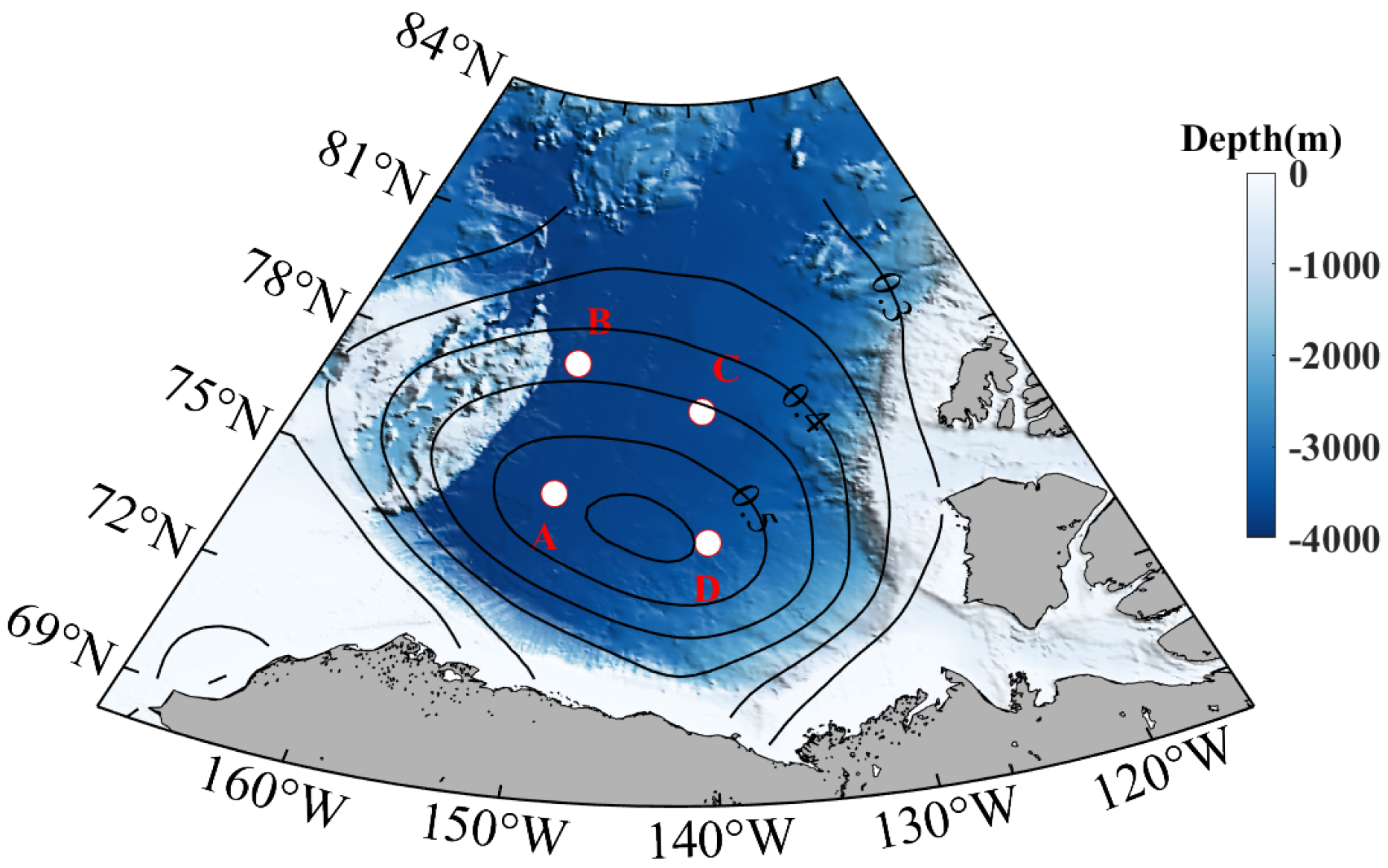
Figure 1. Map of the Arctic Ocean showing its major topographic features. Beaufort Gyre Freshwater experiment mooring locations are marked by white dots and labeled with A, B, C, and D, respectively. The mean surface absolute dynamic topography is shown as black contour lines reflecting the Beaufort Gyre.
Jmse 12 00290 g001
Figure 2. A typical MMP profile recorded at station D at 6 a.m. on 19 November 2006. (a) Potential temperature and salinity (θ-S) diagram. The black dashed lines represent the potential density anomaly (kg/m3). (b) The θ and S profiles with depth. Balck and red line represent θ profile and S profile, respectively. The AW and LHW are denoted with arrows in (a,b). (c) Partial enlargement of the figure (b), the solid circle is the identified θ and S within mixed layer. Balck and red line represent θ profile and S profile, respectively.
Jmse 12 00290 g002
Figure 3. The salinity–time (S-Time) at the four mooring stations during the observation period. (a), (b), (c) and (d) corresponding to station A, B, C and D, respectively. The blank parts indicate that there are no data during these periods.
Jmse 12 00290 g003
Figure 4. The variations in the AW core and LHW core with time at stations A–D. (ac) The variations in the potential temperature, salinity, and depth in the AW core. (df) The corresponding variations in the LHW core.
Jmse 12 00290 g004
Figure 5. The time series of density ratios (a) and buoyancy frequencies (b) defined by AW and LHW at stations A–D.
Jmse 12 00290 g005
Figure 6. PDF of heat flux: FHc_C (black line) and FHc_D (gray line) across the DC staircases at stations C and D. The red and cyan lines represent the lognormally fits for the PDF of FHc_C and FHc_D, respectively.
Jmse 12 00290 g006
Figure 7. PDF of the effective vertical diffusivities: KT_C (black line) and KT_D (gray line) at station C and D. The blue line represents the lognormal fit for the PDFs of KT_C and KT_D.
Jmse 12 00290 g007
Figure 8. The time-series potential temperature of Pacific Winter Water at stations A–D.
Jmse 12 00290 g008
Figure 9. The variation in potential temperature difference between AW and LHW at the stations C (black) and D (gray).
Jmse 12 00290 g009
Table 1. Data description of MMP profiles.
MMP DataABCD
Location75° N, 150° W78° N, 150° W77° N, 140° W74° N, 140° W
TimeAugust 2003–June 2006
August 2007–July 2008
October 2009–July 2011
August 2003–September 2010August 2003–August 2008August 2005–August 2011
Profile number1578196712961896
Disclaimer/Publisher’s Note: The statements, opinions and data contained in all publications are solely those of the individual author(s) and contributor(s) and not of MDPI and/or the editor(s). MDPI and/or the editor(s) disclaim responsibility for any injury to people or property resulting from any ideas, methods, instructions or products referred to in the content.

