
Dynamic Positioning Control of Large Ships in Rough Sea Based on an Improved Closed-Loop Gain Shaping Algorithm


1
Navigation and Ship Engineering College, Dalian Ocean University, Dalian 116023, China
2
Navigation College, Dalian Maritime University, Dalian 116023, China
*
Author to whom correspondence should be addressed.
J. Mar. Sci. Eng. 2024, 12(2), 351; https://doi.org/10.3390/jmse12020351
Submission received: 15 January 2024
/
Revised: 4 February 2024
/
Accepted: 10 February 2024
/
Published: 18 February 2024
(This article belongs to the Special Issue Motion Control and Path Planning of Marine Vehicles—2nd Edition)
Abstract
:In order to solve the problem of the dynamic positioning control of large ships in rough sea and to meet the need for fixed-point operations, this paper proposes a dynamic positioning controller that can effectively achieve large ships’ fixed-point control during Level 9 sea states (wind force Beaufort No. 10). To achieve a better control effect, a large ship’s forward motion is decoupled to establish a mathematical model of the headwind stationary state. Meanwhile, the closed-loop gain shaping algorithm is combined with the exact feedback linearization algorithm to design the speed controller and the course-keeping controller. This effectively solves the problem of strong external interferences impacting the control system in rough seas and guarantees the comprehensive index of robustness performance. In this paper, three large ships—the “Mariner”, “Taian kou”, and “Galaxy”—are selected as the research objects for simulation research and the final fixing error is less than 10 m. It is proven that the method is safe, feasible, practical, and effective, and provides technical support for the design and development of intelligent marine equipment for use in rough seas.
1. Introduction
Dynamic positioning (DP) is an indispensable key technology in the field of ship automation. This function enables a ship to use its own propulsion device to resist the influence of wind, waves, currents, and other external disturbances, as well as maintain a certain attitude at a target position or follow a given trajectory accurately, to complete various operations at sea. The advantages of DP are good maneuverability, easy operation, high positioning accuracy, no damage to the seabed, etc. [1].
Compared with a traditional mooring positioning system, dynamic positioning control uses a network control system (NCS), reducing the design complexity. It is low-cost and easy to expand [2]. However, due to the bandwidth limitation of the network control system, a dynamic positioning task will have a large impact on the control performance of the ship [3]. To address the above problems, scholars have proposed many methods to compensate for errors or suppress interference, aiming to improve the control performance of dynamically positioned ships. Tutturen [4] designed a dynamic positioning controller based on the proportional integral derivative (PID) algorithm, applying conventional PID regulation when close to the desired value and extensive numerical parameter regulation for the remaining operating states. Zhou [5] applied PID control algorithms to design a dynamic positioning system suitable for fully driven autonomous underwater vehicles (AUVs) with predictive compensation for disturbances, thus improving the system stability. Nevertheless, a traditional PID algorithm cannot meet the requirements of ship modeling if external high- and low-frequency interferences are considered. To solve this problem, Jayasiri [6] proposed a wavelet multiresolution-based PID control algorithm to decompose external errors into different frequency bands and then designed PID controllers to solve them separately.
However, the above PID control strategy can only be applied to linear systems and requires that the model is accurately understood. Large ships require nonlinear systems with high control accuracy, so this method is not applicable. To achieve the dynamic positioning of large ships, scholars have conducted further studies into solutions to the model uncertainty problem of complex systems, opening up new avenues in dynamic positioning control. Li [7] determined the model’s parameters by designing a nonlinear observer, and constructed a mathematical model with the particle swarm optimization algorithm, verifying the accuracy of the designed controller’s positioning in the system through a simulation. Tong [8] combined a ship’s high-frequency and low-frequency motion models, as well as mathematical models of wind, waves, currents, thrusters, etc., and designed a comprehensive motion model. With an in-depth study of Kalman filtering technology, the control system solves the problems of phase lag, poor filtering performance and poor control performance due to the existence of low-pass filters. Yu [9] designed a dynamic positioning control system with a linear quadratic Gaussian (LQG) controller to observe a ship’s motion under external wind and wave disturbances using Kalman filtering, proving the feasibility of the method. Cho [10] separated low-frequency motions of ship models using an extended Kalman filter. Moreover, a dynamic positioning sliding mode controller was designed using the Lyapunov theory, and its effectiveness was verified by numerically evaluating the performance of the control algorithm.
The motion equations of a ship at sea are a series of nonlinearly coupled equations. Thus, the above method still has some computational biases, and its positioning accuracy can be further improved. Many scholars have conducted research to solve the problem of using highly linearized equations for ships. Guan [11] designed a controller using the sliding mode variable structure control method, and a stability analysis based on the Lyapunov function exhibited good control performance. Mu [12] considered unknown time-varying disturbances and restricted operating areas, using a fixed-time extended state observer (FDESO) to observe the total perturbation and incorporating the thruster system’s dynamics equations into the controller. The above control methods are robust for nonlinear systems with uncertain perturbations, but, at the same time, they introduce a tremor—a problem that can increase mechanical losses in a propulsion system. Guo [13] utilized an adaptive triggering mechanism to study the DP problem in relation to autonomous surface vehicles (ASVs). A time-varying drift-angle-based heading guidance law using a position error dynamics model and a reduced-order extended state observer was proposed, which performs path-tracking control for ASVs in shallow water environments. Zhang [14] proposed a robust neural event-triggered control algorithm that incorporates dynamic surface control techniques to solve the model’s uncertainty and “complexity explosion” problems, verifying the feasibility of the algorithm with simulation experiments. Bidikli [15] applies adaptive control theory to solve the parameter uncertainty problem, backstepping algorithms to design controllers for the dynamic positioning control of USVs, and the Lyapunov function to verify the system’s stability.
The above research improves the accuracy of dynamic positioning control and solves the problem of highly linearized equations for the motion of ships. However, the results of dynamic positioning studies in rough sea disturbances have not been given. Nowadays, the requirements for marine equipment are strict, so the motion control of ships in rough sea has become a further research direction for scholars. Wei [16] considered external wave force disturbances and other disturbances using control theory and proposed a composite hierarchical anti-disturbance control strategy to realize dynamic positioning control under external environmental disturbances. Su [17] considered complex external disturbances, and constructed an exponential convergence disturbance observer to approximate the external disturbance. Combined with the auxiliary control law of the hyperbolic tangent function, the dynamic positioning control law was designed and proved its effectiveness via simulations. Tomera [18] considered unknown time-varying environmental disturbances and applied the backstepping technique to design a dynamic positioning system; the simulation proved that the proposed controller is effective against external environmental disturbances.
Motivated by the above discussion, this paper focuses on emphasizing the problem of dynamic positioning fixation control for large ships in rough sea conditions. Unlike existing research, the authors introduce rough sea states and consider wind and wave disturbances in Level 9 sea states. Three large ships are selected for simulation experiments to verify the feasibility and generalization of the designed system. Furthermore, large ships are more sensitive to external wind and wave disturbances, thus requiring more accurate controllers to meet their positioning control needs. The main contributions of this research are reflected in the following aspects:
- (1)
- Introduced the equivalent ship speed model and analyzed the conversion relationship between relative wind and absolute wind, based on which, the ship’s headwind stationary motion model was established. This model effectively showed that large ships remain stationary at sea under the interference of external wind and waves. The model plays an important role in the research of dynamic positioning fixed-point control.
- (2)
- The forward speed controller was designed by using the closed-loop gain shaping algorithm, and the nonlinear course-keeping robust controller was designed by combining the closed-loop gain shaping algorithm and the exact feedback linearization algorithm. To overcome the influence of strong external interference on the stability of the system, and thus to meet the demand for fixed-point control, the author decoupled the ship motion and designed the dynamic positioning system using the forward speed controller with the nonlinear course-keeping robust controller. This effectively solved issues with the large-ship control effect in rough seas not being ideal and the result being easy to disperse, and accomplished large-ship fixed-point control at sea.
The remainder of this work was organized as follows: In Section 2, the mathematical modeling of the ship dynamic positioning control system is introduced. The absolute and relative wind conversion model, the equivalent ship speed model, and the ship kinematics model are established. Section 3 shows the design of a speed controller and a nonlinear course-keeping robust controller based on an improved closed-loop gain-shaping algorithm, to realize dynamic positioning control for large vessels. Section 4 presents the basic parameters of three different types of large ships and the overall design of the dynamic positioning task. Section 5 carries out simulation validation in rough sea interference conditions. Section 6 concludes the entire work.
2. Establishment of Mathematical Model for Ship Dynamic Positioning System
2.1. Wind Disturbance Force Model in Rough Sea
Rough sea environments are a specific environmental condition used in this paper to research the task of large ship dynamic positioning control, which in the field of ship control science, mainly refers to class 8–10 sea states [19]. Constructing an accurate disturbance model of the marine environment is one of the necessary tasks for conducting simulation tests of ship control systems. This paper simulates the fixed-point control of a large ship under a level-9 sea state, and set the external wind force to Beaufort No. 10, and the sea wave disturbance to wind-driven wave. The research object is the large ship, and focuses only on wind characteristics in a two-dimensional horizontal plane, i.e., wind speed and wind direction. Due to the influence of ship speed during navigation, the wind speed and wind direction felt on the ship are different from the actual situation. In this paper, the winds under actual conditions are called absolute winds, and the winds to which the ship is subjected during its voyage are called relative winds. The representation of the absolute and relative winds is shown in Figure 1. To establish an absolute wind and relative wind conversion model to represent the ship’s external wind interference more accurately, this model was used to find the relative wind speed and relative wind direction.
The absolute wind speed is UT, the absolute wind angle is , and the range of is 0°–360°, taking the north wind as 0° and the south wind as 180°. The relative air velocity is , the relative wind angle is , and the range of is −180°–180° ( when the wind is blowing from the port side, and when it is blowing from the starboard side). The ship’s speed is , and the relationship between the absolute wind speed, ship speed, and relative wind speed is shown in Equation (1) [20]:
where are two components of the relative wind speed, and the conversion relationship between the relative wind speed and absolute wind speed can be further expressed as Equation (2):
where is the drift angle of a ship, which through trigonometry gives Equation (3):
2.2. Equivalent Ship Speed Model
The equivalent ship speed refers to the normal sailing speed with the same rudder effect when the ship reaches the headwind stationary state under the condition of external wind interference. Considering that an equivalent ship speed model can reflect the rudder efficiency in the simulation, the equivalent ship speed model can be obtained by equating the effective velocity of the inflow rudder at the equivalent ship speed with the effective velocity of the inflow rudder at the ship headwind stationary state [20].
First, calculate the effective velocity of the inflow rudder in the headwind stationary state of the ship [20]; according to the momentum theorem, the fluid momentum change rate of the front and rear of the propeller is equal to the sum of the external forces acting on the fluid. In this paper, the external force acting on the fluid is only the thrust of the propeller:
where is the incoming velocity at the propeller, expressed by Equation (5). and are the axially induced velocities at the paddle disk and at infinity behind the paddle. is the sea water density and the area of the propeller is . The axial induced velocity of the propeller is shown in Equation (6):
where the propeller speed is and the propeller pitch is . is the forward speed of the ship and is the wake coefficient at the propeller. The growth coefficient is shown in Equation (7); it is a function reflecting the distance from the propeller to the rudder.
where is the propeller diameter, when the ship is in a headwind stationary state, the incoming velocity at the propeller is . From Equation (4) to Equation (7), the headwind stationary state into the rudder of the water flow velocity can be obtained as:
Next, assuming that the ship’s equivalent ship speed is , the effective velocity into the rudder [20] can be calculated as shown in Equation (9):
Substituting the equivalent ship speed from Equations (5), (6), and (9), the effective velocity of the inflow rudder at this time can be obtained as:
The mathematical model for the equivalent ship speed V can be found by combining Equations (8) and (10) into Equation (11):
2.3. Ship Kinematics Model
Since the conditions studied in this paper require the inclusion of nonlinear forces as well as wind and wave disturbances in the mathematical model, a third-order Nomoto model before order reduction is adopted:
where K0 is the gain coefficient of the ship model and , , are the ship model time constants. Converting this transfer function to a state space expression, in order to facilitate the inclusion of wind and wave disturbances, matrix transformations according to the Hankel norm and equilibrium realization definitions [21,22] can derive the standard form mathematical model in Equation (13):
where is the rudder, , is the forward speed, is the surging speed, and is the yaw speed of the ship, , is in Equation (14):
In order to facilitate the design of the ship’s speed controller, the mathematical model of the ship’s forward motion needs to be considered separately. The forward motion model can be derived from the linear mathematical model of the plane motion [23]:
where is a first order minor preserved in the hydrodynamic expansion into a Taylor series, is mass of the ship, and , are fluid dynamic derivatives. In the headwind stationary state of the ship, the inertial force term of the fluid is neglected, and the viscous force term of the fluid represents the speed change. The propeller thrust generated is not balanced with the ship’s drag, so the forward motion model can be expressed by the difference between the propeller thrust and the wind force:
where is the thrust of propeller, is the wind force, and is the wave force.
3. Dynamic Positioning Controller Based on Closed-Loop Gain Shaping Algorithm
3.1. Design of Speed Controller
The core of the closed-loop gain shaping algorithm is the direct construction of the closed-loop transfer function matrix and for the design of the controller, where S is the sensitivity function and T is the penalty-sensitivity function. As shown in Figure 2, this can be expressed by Equation (17):
In Figure 2, is the low frequency interference, is a low pass transfer function, is the measurement noise, r is the reference input, y is the actual output, and is the measured output. The sensitivity curve of and is shown in Figure 3. In order to make the system stable, the closed-loop spectrum must be low-pass. The control performance of the system depends on the selection of the crossover frequency, and the closing slope (high frequency asymptote slope) is generally , , and . Then taking the singular value curve of , it is approximated as the spectrum curve of a first-order, second-order, or third-order inertial systems. Furthermore, the controller is deduced inversely [21]:
In this paper, the speed controller is designed by setting the closing slope of the closed-loop transfer function spectrum at . Furthermore, the singular value curve of the closed-loop transfer function can be expressed as the spectrum curve of the third-order inertial system. The speed controller is in Equation (18):
where is the mathematical modeling of the ship forward motion, and the design time constant is based on the bandwidth frequency. Let in Equation (16) be the disturbance force, propeller thrust , and is the propeller thrust factor. From the open-water characteristic curve of the propeller, it can be obtained that [20]. Substituting the propeller thrust into Equation (16), the forward motion model of the ship can be obtained as follows:
substitute Equation (19) into Equation (18) to obtain the speed controller Equation (20):
3.2. Design of the Nonlinear Course-Keeping Robust Controller
Since the influence of rough seas is considered in this paper, conventional course-keeping controllers based on closed-loop gain shaping algorithms are not able to effectively eliminate strong external disturbances, which in turn cannot guarantee the robust performance and robust stability of the system [24,25]. Considering this problem, the author combines a closed-loop gain shaping algorithm with an exact feedback linearization algorithm for a dynamic positioning controller design. Firstly, the closed-loop gain shaping algorithm is used to complete the design of the course-keeping control law, and then the precise feedback linearization algorithm is used to complete the design of the nonlinear course-keeping robust control law to ensure the robust stability of the dynamic positioning systems in rough sea disturbances.
The course-keeping controller is designed by the closing slope of the closed-loop transfer function spectrum being set at , and the singular value curve of the closed-loop transfer function can be expressed as the spectrum curve of the second-order inertial system. The course-keeping controller can be obtained as:
where is the ship Nomoto motion model and the design time constant , based on the bandwidth frequency. It can be seen from reference [26] that the essence of exact feedback linearization control is to eliminate the nonlinear part first, and then to add the linearized control rate. Considering the reduced-order Nomoto model, since the research object is a static unstable ship, the second term at the left end of the reduced-order Nomoto model needs to be replaced by the nonlinear [27]. By introducing the third-order term, the nonlinear situation of the system response can be better fitted. Currently, the designed nonlinear function is as shown in Equation (22):
Combining Equations (21) and (22), the nonlinear course-keeping robust controller can be derived as:
where , are nonlinear parameters and , are ship maneuverability indices.
4. General System Design
In order to verify the fixed-point control effect of the designed ship dynamic positioning controller for large ships in rough sea conditions, in this paper, three large ships—the “Taian kou”, “Mariner”, and “Galaxy”—were selected for simulation research. Their ship parameters are shown in Table 1. The mathematical model of the controlled object is the ship’s headwind stationary motion model derived from computational analysis. The specific model construction was elaborated in Chapter 1 of this paper.
The system simulation block diagram based on the designed nonlinear course-keeping robust controller and speed controller, as shown in Figure 4.
Where negative feedback function is the designed nonlinearization function, the saturation and integral terms are the ship’s host characteristics. The input wind direction in the simulation block diagram is the set target wind chord angle, and the input speed is the wave speed under wind-driven wave conditions. The overall technical roadmap of the system is shown in Figure 5.
Separate rotary tests on three large ships, taking the yaw angular velocity after reaching steady state as , were performed. By fitting the relationship by the least squares method, the maneuverability indices of the three ships as well as the nonlinear parameters were obtained, as shown in Table 2.
5. Simulation Verification and Results Analysis
In this paper, the simulation research of the initial state of the ship is static, the ship’s heading is 0° and the initial position of the ship is . In view of the rough sea environment, wind and wave interference were added to the system. The specific parameters were wind force Beaufort No. 10 (wind speed 27 ) and wind direction 40°. The wave was a wind-driven wave, and its three-dimensional model simulation diagram is shown in Figure 6. Applying the designed dynamic positioning controller, the controlled ship adjusted its heading, and finally kept the headwind stationary. Firstly, the curves of the heading change and forward speed of the “Taian kou” ship with time are shown in Figure 7.
It can be seen from Figure 7 that, because of the influence of strong external interference, the speed of the simulation was larger at the beginning of the simulation. Then, the heading quickly turned to 40° and the forward speed tended to 0 and oscillated slightly near 0 . Furthermore, the rapid fixed-point control was achieved in less than 100 s. The curves of the heading change and forward speed of the “Mariner” ship with time are shown in Figure 8.
It can be seen from Figure 8 that the heading of the “Mariner” ship turned to 40° in less than 160 s. The ship reached a headwind stationary state, which meets the demands of fixed-point control. The curves of the heading change and forward speed of the “Galaxy” ship with time are shown in Figure 9.
It can be seen from Figure 9 that the heading of the “Galaxy” ship turned to 40° in less than 400 s. This proves that it can quickly reach a steady state with good control performance.
From the simulation results of the three large ships, the dynamic positioning control system designed in this paper was able to effectively overcome strong external interferences under a level-9 sea state, and all ships were able to quickly maintain the headwind stationary state. In order to further verify the fixed-point control effect of the designed dynamic positioning control system, simulation research on the center of gravity trajectories of the three ships under wind force Beaufort No. 10 and wind direction 40° were carried out. The center of gravity trajectories of the three large ships are shown in Figure 10.
The initial heading of the ships was 0° and the initial position of ship was . From the simulation results in Figure 6 to Figure 9, the ship had a large forward speed impulse under the influence of the strong wind at the beginning of the simulation. Then, it decreased rapidly in a very short time and tended towards the normal traveling speed, and the heading of the ship also changed drastically with the strong wind. As the simulation proceeded, the ships’ rudder efficiency gradually became better under the action of the designed dynamic positioning controller. The bow quickly turned towards the windward state and stabilized at the headwind angle. Furthermore, the oscillation amplitude of the ship’s forward speed curve gradually decreased and tended towards 0 within 100 s, maintaining the headwind stationary state. The reference and actual values of the heading angle and forward speed of the three large ships are shown in Table 3.
The center of gravity trajectories of the three ships could also be more intuitively seen from the ship’s fixed-point control effect under the designed dynamic positioning control system; the same simulation time of the three ships finally completed the fixed-point control task. The “Mariner” ship’s fixed-point distance from the initial position was maintained within 10 m, the “Taian kou” ship’s fixed-point distance from the initial position was maintained within 5 m, and the “Galaxy” ship’s fixed-point distance from the initial position was maintained within 7 m. Finally, the three large ships’ fixed-point distance from the initial position was maintained within 10 m, and the fixed-points were effective and met the fixed-point control requirements.
6. Conclusions
This paper addresses the large-ship problem of fixed-point control for dynamic positioning in rough sea conditions. Through theoretical analysis and simulation experiments, we made the following conclusions:
- (1)
- We built a stationary motion model of ship headwind by introducing an equivalent ship speed model and analyzing the conversion relationship between the relative wind and absolute wind. The model effectively showed the large ship overcoming strong external disturbances and remaining stationary at sea, providing good modeling support for research into large ship fixed-point control in rough sea conditions.
- (2)
- In order to overcome strong external disturbances at a level-9 sea state, the authors decoupled the ship motions and built a mathematical model. Combining the closed-loop gain shaping algorithm with an exact feedback linearization algorithm to design a nonlinear course-keeping robust controller, the designed dynamic positioning control system combined a ship speed controller with a nonlinear course-keeping robust controller. The simulation results proved that the fixed-point control errors of the three ships were all less than 10 m, which meets the fixed-point control requirements of large ships in rough sea conditions.
The method proposed in this paper can provide technical support for the dynamic positioning control of large ships in rough sea conditions. In the future, the authors will continue to conduct research on dynamic positioning trajectory control or on-line control for large ships under changing sea states or phenomenal sea states; this plays an auxiliary role in the construction of marine-ship dynamic-positioning intelligent equipment.
Author Contributions
Conceptualization, C.S. and X.Z.; methodology, X.Z.; software, C.S.; validation, C.S. and J.S.; formal analysis, T.G.; investigation, T.G.; resources, J.S. and X.Z.; data curation, T.G.; writing—original draft preparation, C.S. and T.G.; writing—review and editing, C.S. and J.S.; visualization, C.S.; supervision, J.S. and X.Z.; project administration, J.S.; funding acquisition, J.S.; All authors have read and agreed to the published version of the manuscript.
Funding
This research received no external funding.
Institutional Review Board Statement
Not applicable.
Informed Consent Statement
Not applicable.
Data Availability Statement
If you need to obtain the experimental information and data presented in the paper, please contact the author.
Conflicts of Interest
The authors declare no conflicts of interest.
References
- Zhang, G.Q.; Yao, M.Q.; Yang, T.T.; Zhang, W.D. Ship adaptive dynamic positioning control considering event-triggered input. J. Control Theory Appl. 2021, 38, 1597–1606. [Google Scholar] [CrossRef]
- Du, J.L.; Hu, X.; Krstić, M.; Sun, Y.Q. Robust dynamic positioning of ships with disturbances under input saturation. Automatica 2016, 73, 207–214. [Google Scholar] [CrossRef]
- Zhang, X.M.; Han, Q.L.; Yu, X. Survey on recent advances in networked control systems. IEEE Trans. Ind. Inform. 2015, 12, 1740–1752. [Google Scholar] [CrossRef]
- Tutturen, S.A.; Skjetne, R. Hybrid control to improve transient response of integral action in dynamic positioning of marine vessels. IFAC Pap. 2015, 48, 166–171. [Google Scholar] [CrossRef]
- Zhou, Q.R.; Zeng, Q.J.; Yao, J.Y.; Zhu, Z.Y.; Dai, W.W. Design and implementation of fully-actuated AUV dynamic positioning system. J. Underw. Unmanned Syst. 2019, 27, 333–338. [Google Scholar] [CrossRef]
- Jayasiri, A.; Ahmed, S.; Imtiaz, S. Wavelet-based controller design for dynamic positioning of vessels. IFAC Pap. 2017, 50, 1133–1138. [Google Scholar] [CrossRef]
- Li, J. Application of nonlinear observer in DP of ship dynamic positioning system. Ship Sci. Technol. 2021, 43, 208–210. [Google Scholar] [CrossRef]
- Tong, J.J.; He, L.M.; Tian, Z.H. Mathematical model of ship dynamic positioning system. Ship Eng. 2002, 05, 27–29. [Google Scholar] [CrossRef]
- Yu, P.W.; Chen, H. Design of optimal controller for dynamic positioning system. Adv. Mater. Res. 2011, 308, 2127–2130. [Google Scholar] [CrossRef]
- Cho, S.; Shim, H.; Kim, Y.S. Dynamical sliding mode control for robust dynamic positioning systems of FPSO vessels. J. Mar. Sci. Eng. 2022, 10, 474. [Google Scholar] [CrossRef]
- Guan, K.P.; Zhang, X.F. Research on sliding mode control ship dynamic positioning control system. Ship Sci. Technol. 2018, 40, 61–65. [Google Scholar] [CrossRef]
- Mu, D.D.; Feng, Y.P.; Wang, G.F.; Fan, Y.S.; Zhao, Y.S.; Sun, X.J. Ship dynamic positioning output feedback control with position constraint considering thruster system dynamics. J. Mar. Sci. Eng. 2023, 11, 94. [Google Scholar] [CrossRef]
- Guo, Q.; Zhang, X.K.; Han, X. Robust adaptive event-triggered path following control for autonomous surface vehicles in shallow waters. Ocean Eng. 2023, 286, 115571. [Google Scholar] [CrossRef]
- Zhang, G.Q.; Yao, M.Q.; Xu, J.H.; Zhang, W.D. Robust neural event-triggered control for dynamic positioning ships with actuator faults. Ocean Eng. 2020, 207, 107292. [Google Scholar] [CrossRef]
- Bidikli, B. An adaptive control design for dynamic positioning of unmanned surface vessels having actuator dynamics. Ocean Eng. 2021, 229, 108948. [Google Scholar] [CrossRef]
- Wei, X.J.; Zhang, H.F.; Wei, Y.L. Composite hierarchical anti-disturbance control for dynamic positioning system of ships based on robust wave filter. Ocean Eng. 2022, 262, 112173. [Google Scholar] [CrossRef]
- Su, Y.X.; Gong, C.L.; Zhang, D.H.; Hu, X. Simple Dynamic Positioning Control Design for Surface Vessels With Input Saturation and External Disturbances. IEEE Trans. Circuits Syst. II Express Briefs 2022, 70, 1530–1534. [Google Scholar] [CrossRef]
- Tomera, M.; Podgórski, K. Control of dynamic positioning system with disturbance observer for autonomous marine surface vessels. Sensors 2021, 21, 6723. [Google Scholar] [CrossRef]
- Zhang, G.Q. Simple Robust Adaptive Control of Ship Motion in Severe Sea Conditions. Ph.D. Thesis, Dalian Maritime University, Dalian, China, 2015. [Google Scholar] [CrossRef]
- Jia, X.L.; Yang, Y.S. Mathematical Model of Ship Motion: Mechanism Modeling and Identification Modeling; Dalian Maritime University: Dalian, China, 1999. [Google Scholar]
- Jia, X.L.; Zhang, X.K. Ship Motion Intelligent Control and H∞ Robust Control; Dalian Maritime University: Dalian, China, 2002. [Google Scholar]
- Song, C.Y.; Zhang, X.K.; Zhang, G.Q. Nonlinear identification for 4-DOF ship maneuvering modeling via full-scale trial data. IEEE Trans. Ind. Electron. 2021, 69, 1829–1835. [Google Scholar] [CrossRef]
- Jiang, Z.R. Modeling and Simulation of Control System: Analysis and Implementation Based on MATLAB/Simulink; Tsinghua University: Beijing, China, 2020. [Google Scholar]
- Menini, L.; Tornambè, A. Exact and approximate feedback linearization without the linear controllability assumption. Automatica 2012, 48, 2221–2228. [Google Scholar] [CrossRef]
- Song, C.Y.; Zhang, X.K.; Zhang, G.Q. Nonlinear innovation-based maneuverability prediction for marine vehicles using an improved forgetting mechanism. J. Mar. Sci. Eng. 2022, 10, 1210. [Google Scholar] [CrossRef]
- Zhou, Z.Y.; Zhang, Y.J.; Wang, S.B. A coordination system between decision making and controlling for autonomous collision avoidance of large intelligent ships. J. Mar. Sci. Eng. 2021, 9, 1202. [Google Scholar] [CrossRef]
- Ren, R.Y.; Zou, Z.J.; Wang, Y.D.; Wang, X.G. Adaptive Nomoto model used in the path following problem of ships. J. Mar. Sci. Technol. 2018, 23, 888–898. [Google Scholar] [CrossRef]
Figure 1.
Representation of absolute and relative winds.

Figure 2.
A common closed-loop control loop.
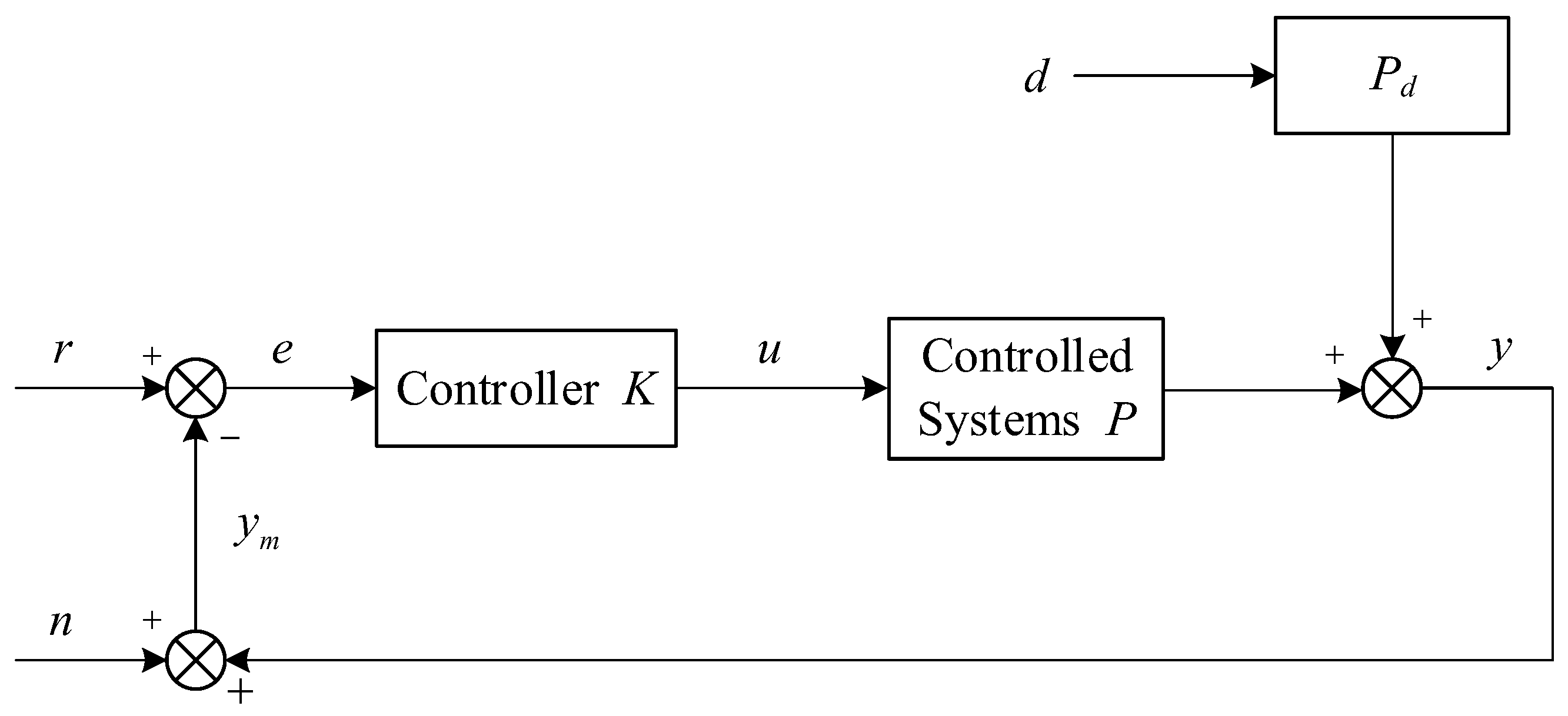
Figure 3.
Expected sensitivity curve.
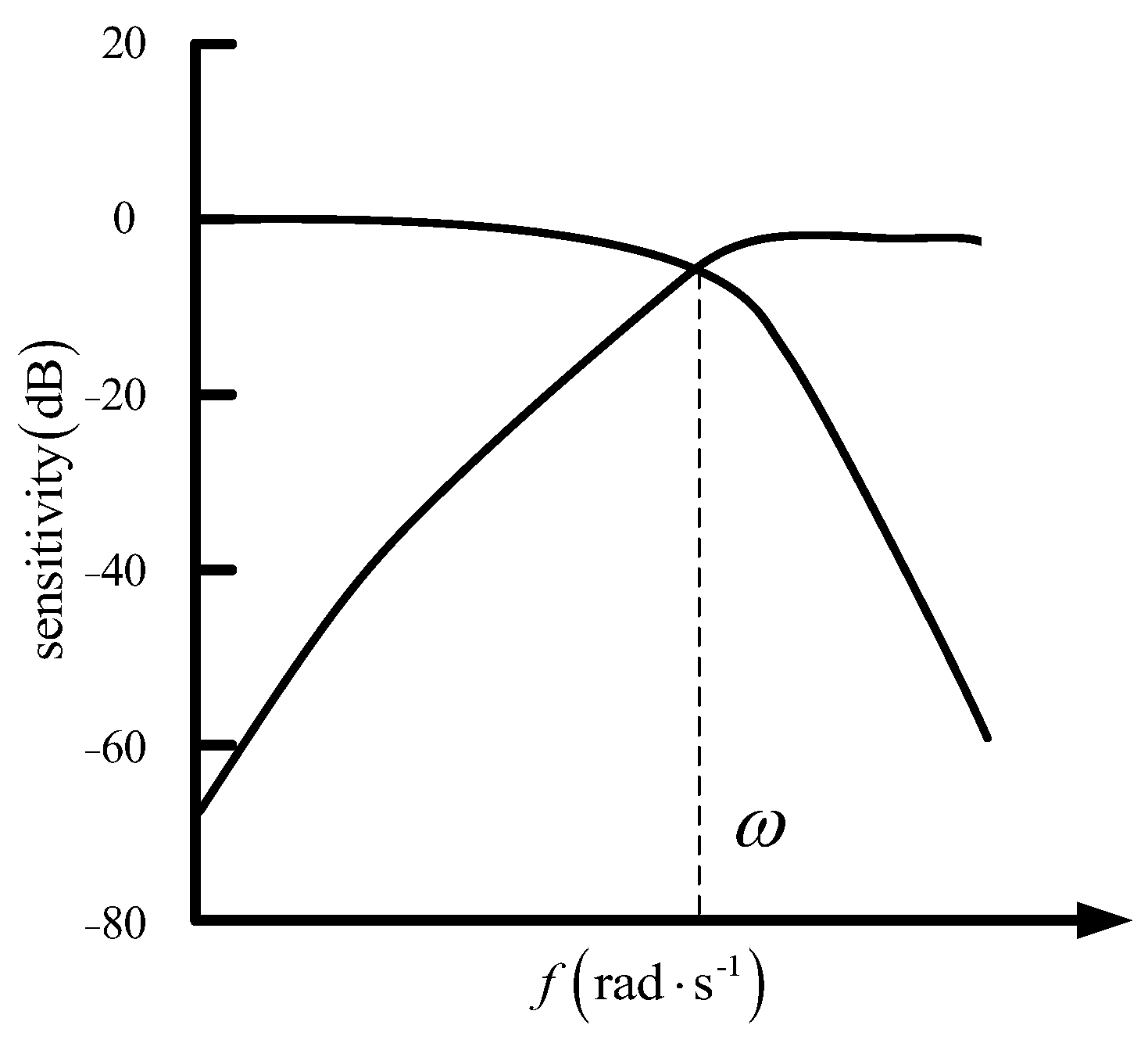
Figure 4.
Schematic block diagram of the control structure.

Figure 5.
System overall technology roadmap.
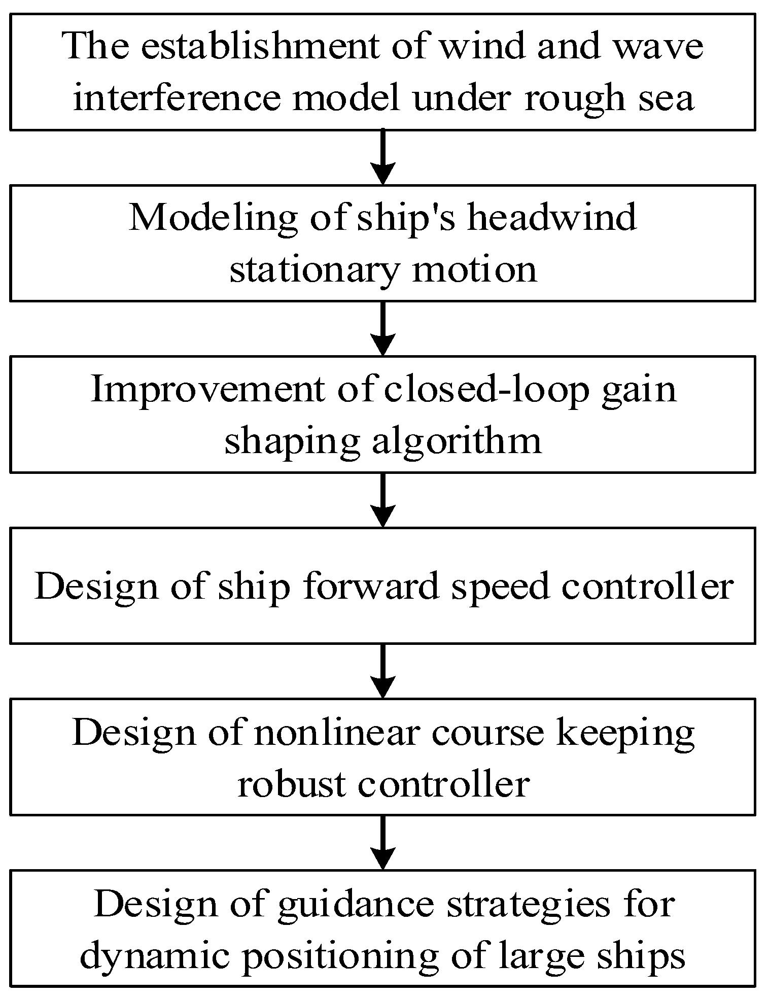
Figure 6.
Three-dimensional simulation view of waves under a level-9 sea state.

Figure 7.
(a) Heading of “Taian kou” ship; (b) Forward speed of “Taian kou” ship.
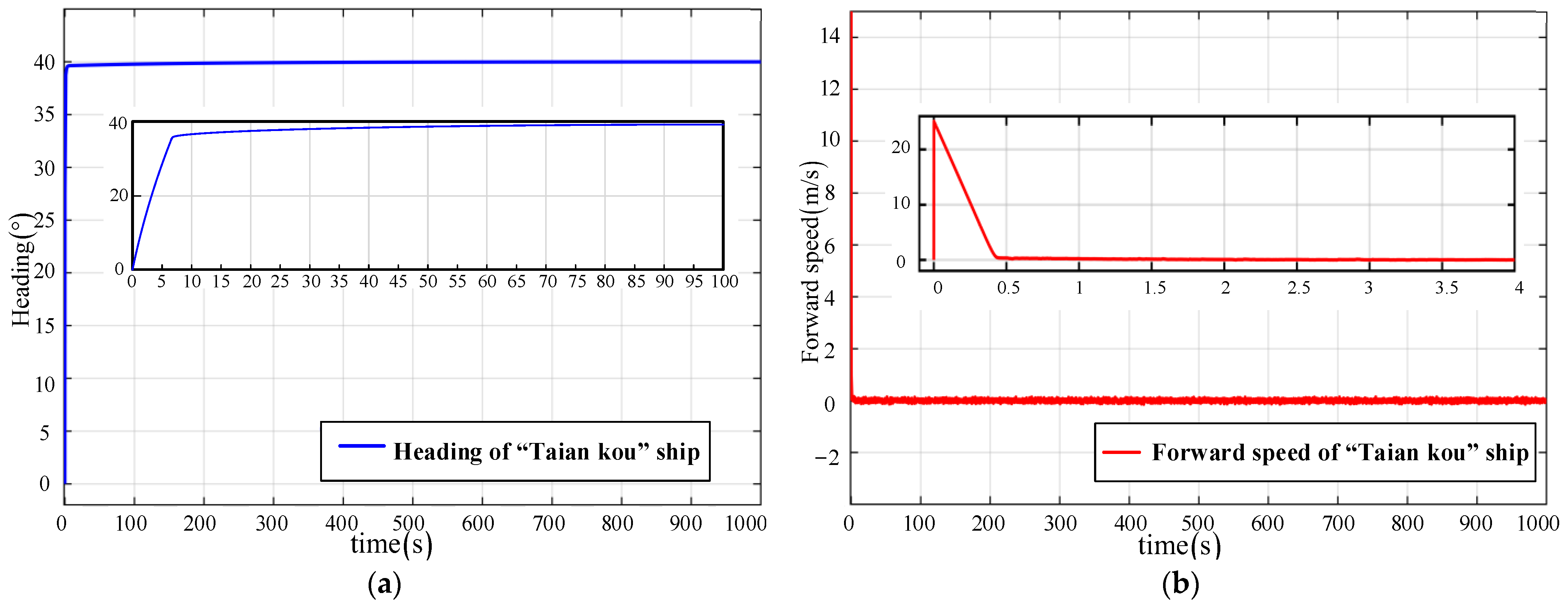
Figure 8.
(a) Heading of “Mariner” ship; (b) Forward speed of “Mariner” ship.

Figure 9.
(a) Heading of “Galaxy” ship; (b) Forward speed of “Galaxy” ship.
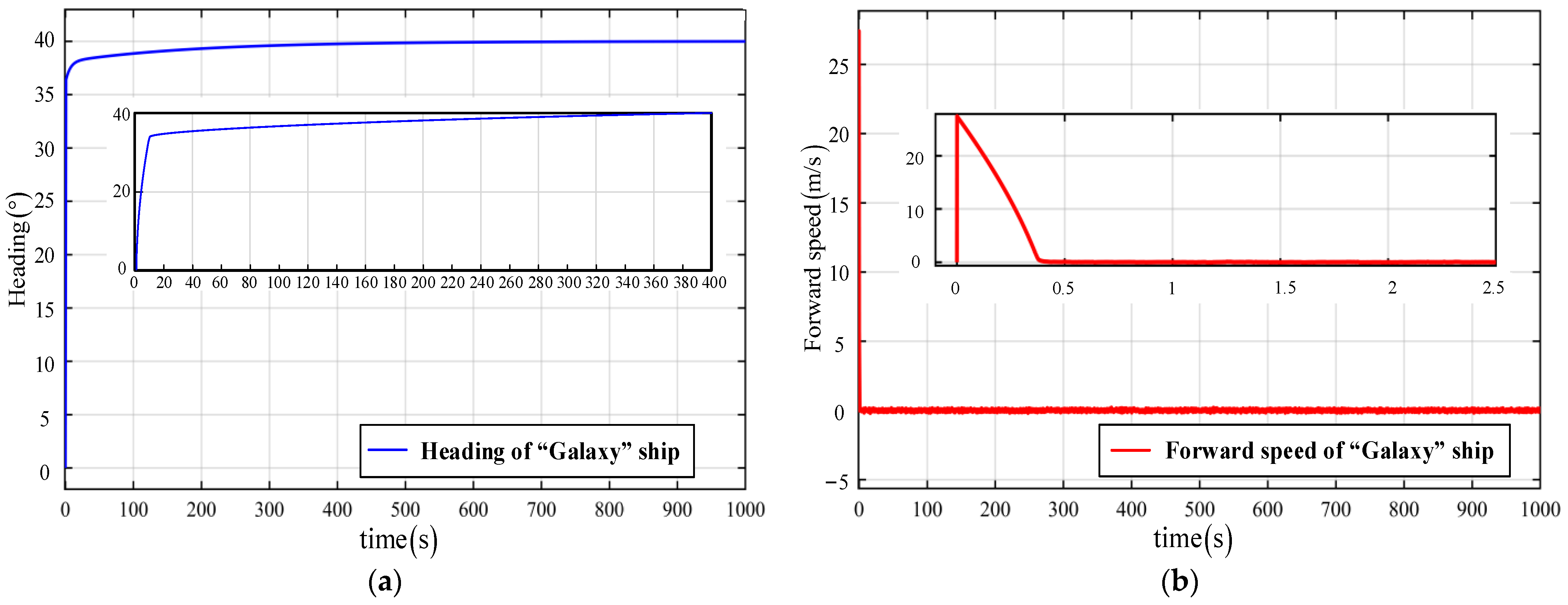
Figure 10.
(a) Center of gravity trajectories of “Mariner” ship; (b) Center of gravity trajectories of “Taian kou” ship; (c) Center of gravity trajectories of “Galaxy” ship.
Figure 10.
(a) Center of gravity trajectories of “Mariner” ship; (b) Center of gravity trajectories of “Taian kou” ship; (c) Center of gravity trajectories of “Galaxy” ship.


Table 1.
Basic parameters of the ship.
| Quantity | Symbol | Value | ||
|---|---|---|---|---|
| “Taian kou” Ship | “Mariner” Ship | “Galaxy” Ship | ||
| Length between perpendiculars | 145.00 | 160.93 | 160.00 | |
| Breadth | 36.00 | 23.17 | 28.00 | |
| Draft | 7.40 | 8.23 | 9.50 | |
| Displacement | 30,881.2 | 19,004.5 | 28,848.6 | |
| Rudder area | 20.4 | 30.1 | 38.9 | |
| Paddle diameter | 4.0 | 6.7 | 6.3 | |
| Block coefficient | 0.787 | 0.558 | 0.652 | |
Table 2.
Ship maneuverability index and nonlinear parameters.
| Ship | Maneuverability Index | Nonlinear Parameter | ||
|---|---|---|---|---|
| K | T | α | β | |
| “Taian kou” ship | −0.20 | −212.96 | 8.94 | 33,624.80 |
| “Mariner” ship | 0.10 | 48.85 | 16.75 | 20,887.82 |
| “Galaxy” ship | 0.48 | 186.82 | 8.87 | 8911.21 |
Table 3.
The reference value and actual values of ship heading and forward speed.
| Ship | Heading | Forward Speed | ||
|---|---|---|---|---|
| Reference Value | Actual Value | Reference Value | Actual Value | |
| “Taian kou” ship | 40° | 40° | 0 | 0 0.3 |
| “Mariner” ship | 40° | 40° | 0 | 0 0.65 |
| “Galaxy” ship | 40° | 40° | 0 | 0 0.8 |
Disclaimer/Publisher’s Note: The statements, opinions and data contained in all publications are solely those of the individual author(s) and contributor(s) and not of MDPI and/or the editor(s). MDPI and/or the editor(s) disclaim responsibility for any injury to people or property resulting from any ideas, methods, instructions or products referred to in the content. |
© 2024 by the authors. Licensee MDPI, Basel, Switzerland. This article is an open access article distributed under the terms and conditions of the Creative Commons Attribution (CC BY) license (https://creativecommons.org/licenses/by/4.0/).
Share and Cite
MDPI and ACS Style
Song, C.; Guo, T.; Sui, J.; Zhang, X. Dynamic Positioning Control of Large Ships in Rough Sea Based on an Improved Closed-Loop Gain Shaping Algorithm. J. Mar. Sci. Eng. 2024, 12, 351. https://doi.org/10.3390/jmse12020351
AMA Style
Song C, Guo T, Sui J, Zhang X. Dynamic Positioning Control of Large Ships in Rough Sea Based on an Improved Closed-Loop Gain Shaping Algorithm. Journal of Marine Science and Engineering. 2024; 12(2):351. https://doi.org/10.3390/jmse12020351
Chicago/Turabian StyleSong, Chunyu, Teer Guo, Jianghua Sui, and Xianku Zhang. 2024. "Dynamic Positioning Control of Large Ships in Rough Sea Based on an Improved Closed-Loop Gain Shaping Algorithm" Journal of Marine Science and Engineering 12, no. 2: 351. https://doi.org/10.3390/jmse12020351
Note that from the first issue of 2016, this journal uses article numbers instead of page numbers. See further details here.