
Mid-Deep Circulation in the Western South China Sea and the Impacts of the Central Depression Belt and Complex Topography
 ,
, 
Abstract
:1. Introduction
2. Data and Methods
2.1. Observation Data
2.2. HYCOM Simulation
2.3. Bathymetric Data
2.4. Richardson Number and Fine-Scale Parameterization
3. Results
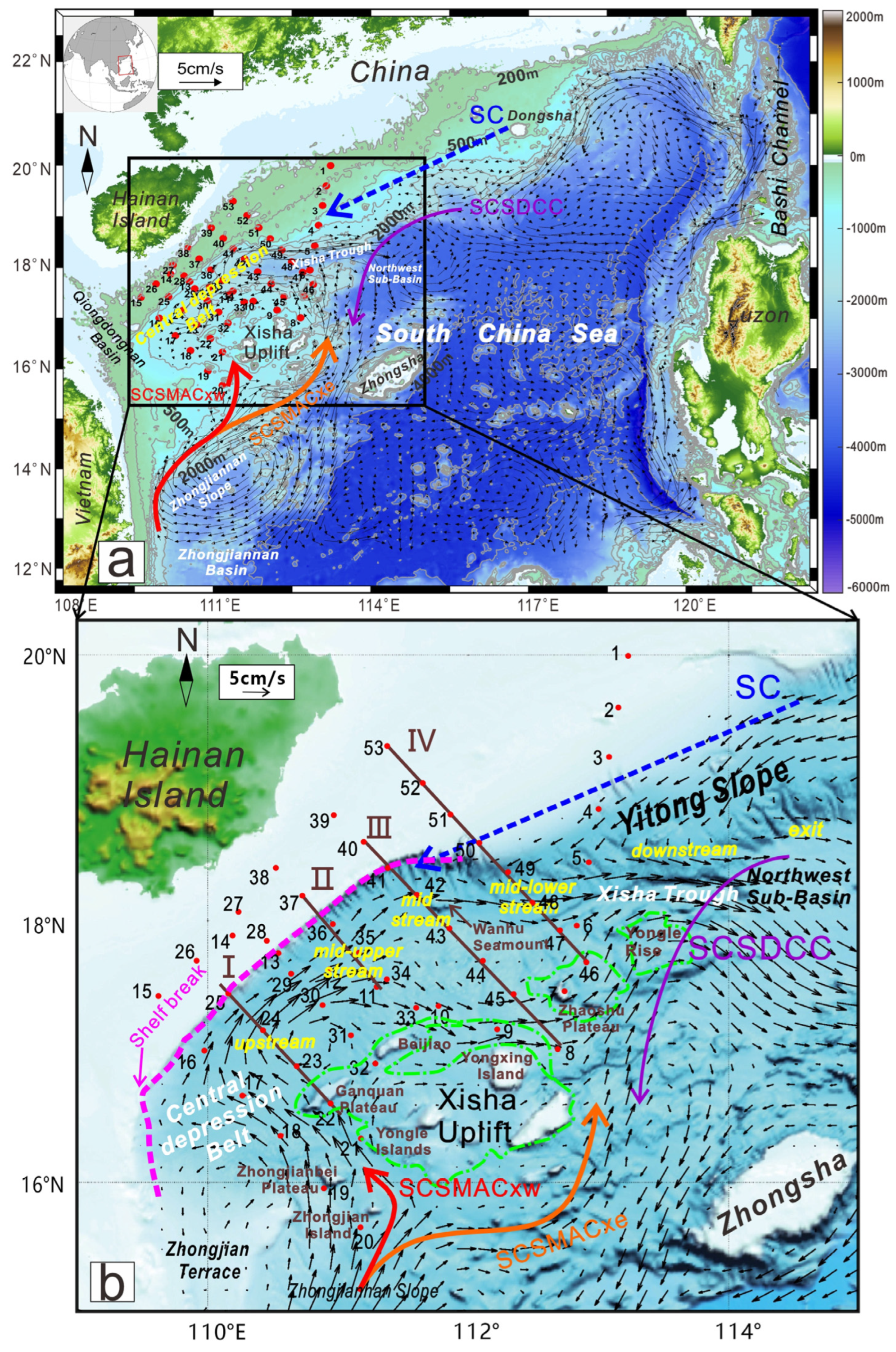
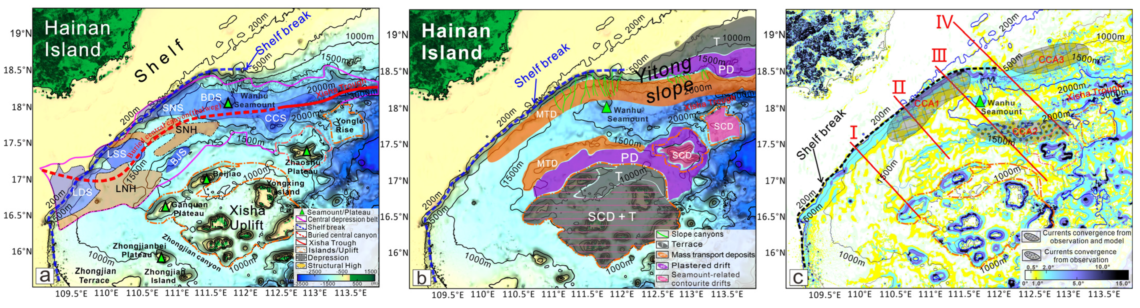
3.1. Geomorphology
3.2. Ocean Dynamics
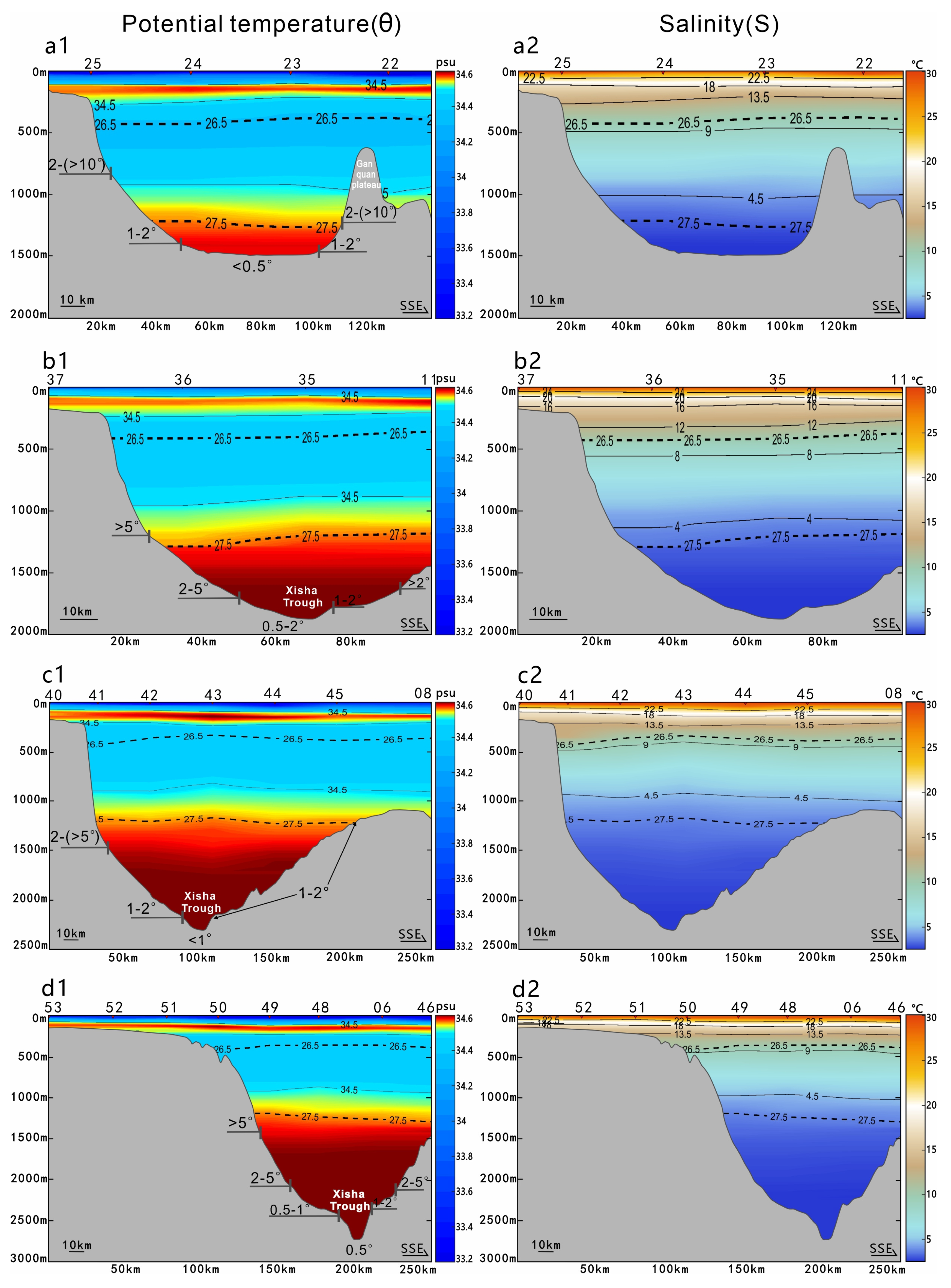
3.2.1. Water Masses
3.2.2. Observational Currents Properties in the Central Depression Belt
3.3. Modeling of Currents around the Central Depression Belt
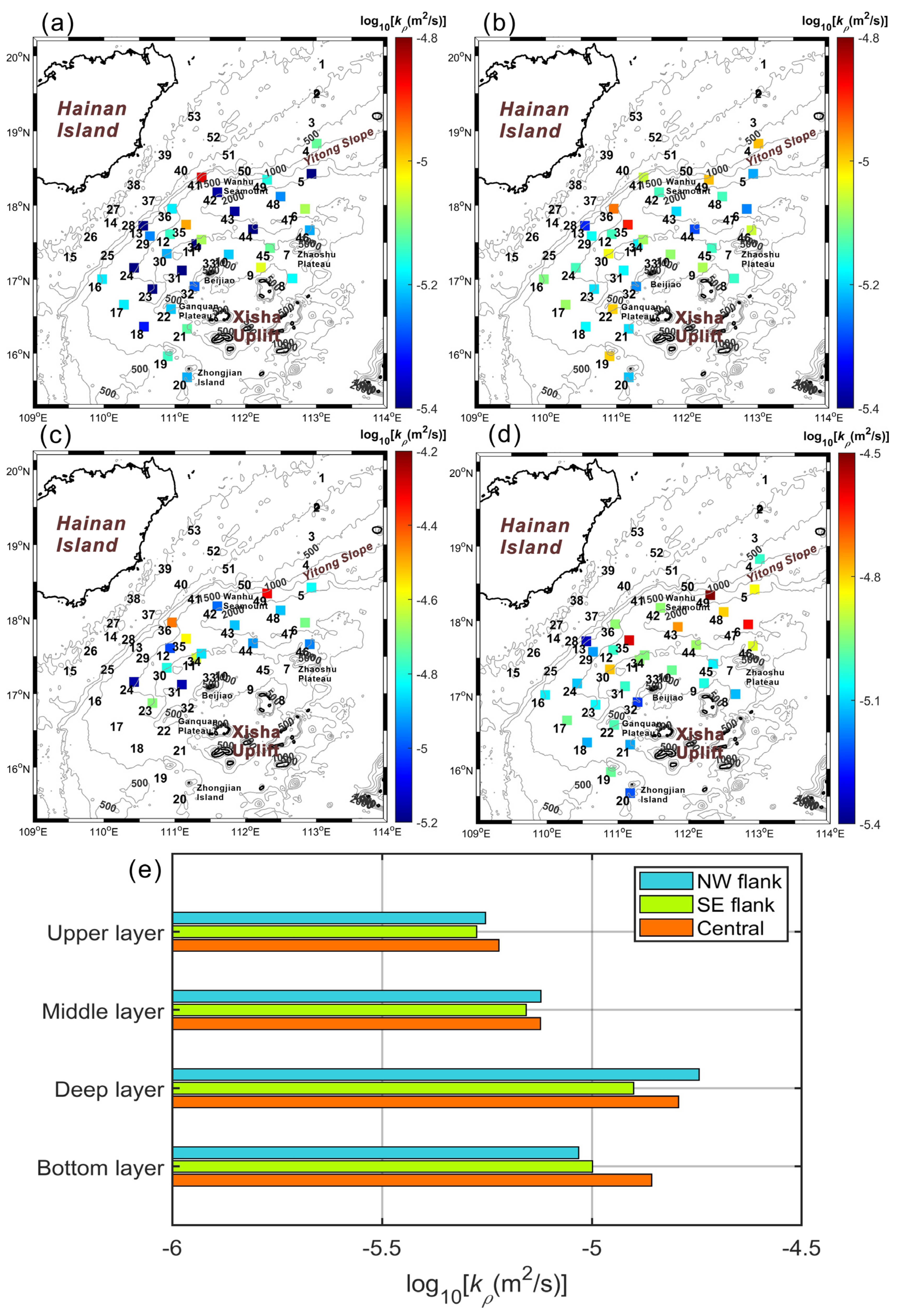
3.4. Horizontal and Vertical Distributions of Turbulence Parameterizations in the Central Depression Belt
4. Discussion
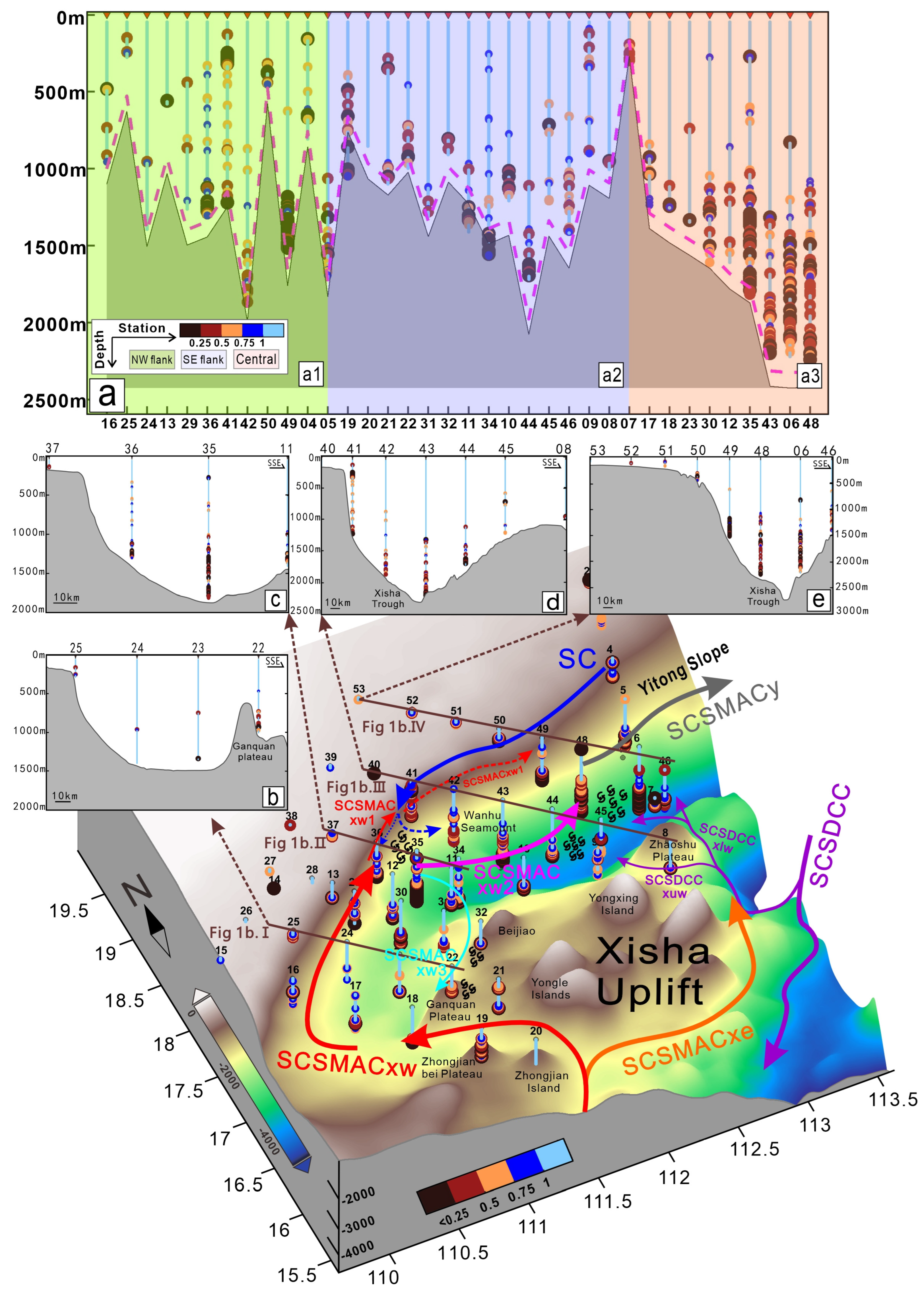
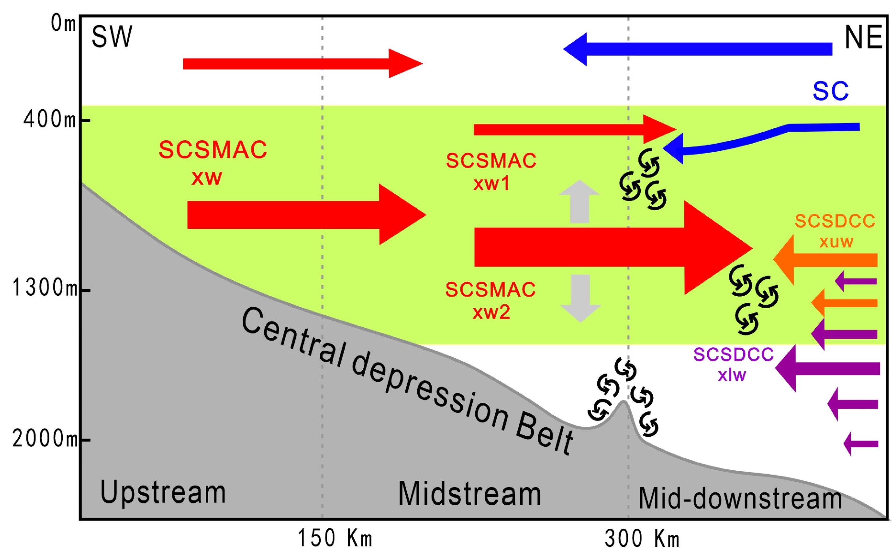
4.1. Mid-Deep Circulation Pattern in the Central Depression Belt
4.1.1. SCSMACxw1 Converges with SC at 300–1000 m
4.1.2. SCSMACxw2 Converges with SCSDCCxuw and SCSDCCxlw at 1000–2000 m
4.2. Factors Affecting the Central Depression Belt Circulation Pattern
4.2.1. Local Wind and Eddies
4.2.2. Seabed Topography Changes
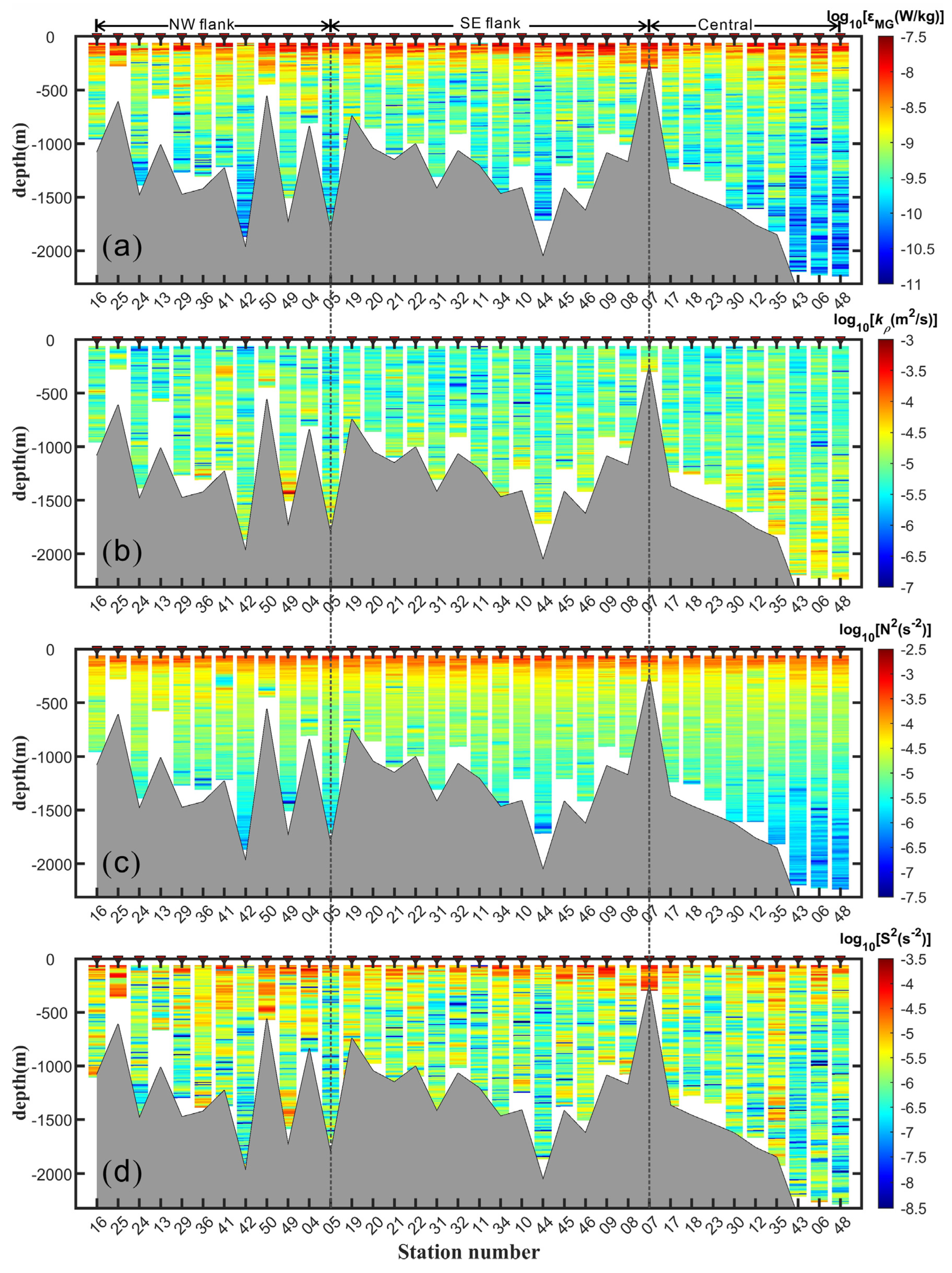
4.3. Enhanced Mixing in the Central Depression Belt
5. Conclusions
- (1)
- (2)
- Over the central depression belt region, seabed topography changes have a decisive impact on developing a local mid-deep circulation pattern, where current intensification is promoted by current–topography interactions. In comparison, winds and mesoscale eddies can substantially affect upper-surface currents while having limited influence in the mid-deep layers.
- (3)
- Inconsistencies between model results and observations correspond to both the apparent lack of intensifications (i.e., velocities, core scopes) for SC and SCSMACxw2. The former is due to the fact that the model underestimates the seasonal variations in the strength and vertical structure of the slope currents along the northwestern margin of the SCS. The latter is because the topographic resolution used in the model (~10 km) is too low to capture the forcing signals of the real seabed topography in the mid-downstream.
- (4)
- Prominent convergence of SCSMACxw1 and SC from ~300 to 1000 m deep and of SCSMACxw2, SCSDCCxuw, and SCSDCCxlw from ~1000 to 2000 m deep significantly change the properties of the relevant currents and water masses (Figure 12). Enhanced local mixing is assigned to the relevant regions above, pointing out the convergence as a dominant mechanism for generating instability.
Supplementary Materials
Author Contributions
Funding
Institutional Review Board Statement
Informed Consent Statement
Data Availability Statement
Acknowledgments
Conflicts of Interest
References
- Eiff, O.S.; Bonneton, P. Lee-wave breaking over obstacles in stratified flow. Phys. Fluids 2000, 12, 1073–1086. [Google Scholar] [CrossRef]
- Wang, D.; Wang, Q.; Zhou, W.; Cai, S.; Li, L.; Hong, B. An analysis of the current deflection around Dongsha Islands in the northern South China Sea. J. Geophys. Res. Oceans 2013, 118, 490–501. [Google Scholar] [CrossRef]
- Naveira Garabato, A.C.; Frajka-Williams, E.E.; Spingys, C.P.; Legg, S.; Polzin, K.L.; Forryan, A.; Abrahamsen, E.P.; Buckingham, C.E.; Griffies, S.M.; McPhail, S.D. Rapid mixing and exchange of deep-ocean waters in an abyssal boundary current. Proc. Natl. Acad. Sci. USA 2019, 116, 13233–13238. [Google Scholar] [CrossRef] [PubMed]
- Kunze, E.; Smith, S.G.L. The role of small-scale topography in turbulent mixing of the global ocean. Oceanography 2004, 17, 55–64. [Google Scholar] [CrossRef]
- Yan, X.; Kang, D.; Curchitser, E.N.; Pang, C. Energetics of Eddy-Mean Flow Interactions along the Western Boundary Currents in the North Pacific. J. Phys. Oceanogr. 2019, 49, 789–810. [Google Scholar] [CrossRef]
- Liu, X.; Wang, D.-P.; Su, J.; Chen, D.; Lian, T.; Dong, C.; Liu, T. On the Vorticity Balance over Steep Slopes: Kuroshio Intrusions Northeast of Taiwan. J. Phys. Oceanogr. 2020, 5, 2089–2104. [Google Scholar] [CrossRef]
- Qiu, C.; Mao, H.; Liu, H.; Xie, Q.; Yu, J.; Su, D.; Ouyang, J.; Lian, S. Deformation of a warm eddy in the northern South China Sea. J. Geophys. Res. Oceans 2019, 124, 5551–5564. [Google Scholar] [CrossRef]
- Su, D.; Lin, P.; Mao, H.; Wu, J.; Liu, H.; Cui, Y.; Qiu, C. Features of slope intrusion mesoscale eddies in the northern South China Sea. J. Geophys. Res. Oceans 2020, 125, e2019JC015349. [Google Scholar] [CrossRef]
- Vilela-Silva, F.; Silveira, I.C.A.; Napolitano, D.C.; Souza-Neto, P.W.M.; Biló, T.C.; Gangopadhyay, A. On the Deep Western Boundary Current Separation and Anticyclone Genesis off Northeast Brazil. J. Geophys. Res. Oceans 2023, 128, e2022JC019168. [Google Scholar] [CrossRef]
- Lee, S.K.; Pelegrí, J.L.; Kroll, J. Slope Control in Western Boundary Currents. J. Phys. Oceanogr. 2001, 31, 3349–3360. [Google Scholar] [CrossRef]
- Stommel, H. The westward intensification of wind-driven ocean currents. Eos Trans. Am. Geophys. Union 1948, 29, 202–206. [Google Scholar]
- Harris, P.T.; Macmillan-Lawler, M.; Rupp, J.; Baker, E.K. Geomorphology of the oceans. Mar. Geol. 2014, 352, 4–24. [Google Scholar] [CrossRef]
- Wu, Z.; Li, J.; Jin, X.; Shang, J.; Jin, X.; Li, S. Distribution, features, and influence factors of the submarine topographic boundaries of the Okinawa Trough. Sci. China Earth Sci. 2014, 57, 1885–1896. [Google Scholar] [CrossRef]
- Holland, W.R. Baroclinic and topographic influences on the transport in western boundary currents. Geophys. Fluid Dyn. 1973, 4, 187–210. [Google Scholar] [CrossRef]
- Spall, M.A. Boundary Currents and Watermass Transformation in Marginal Seas. J. Phys. Oceanogr. 2017, 34, 1197–1213. [Google Scholar] [CrossRef]
- Shu, Y.; Wang, J.; Xue, H.; Huang, R.X.; Chen, J.; Wang, D.; Wang, Q.; Xie, Q.; Wang, W. Deep-Current Intraseasonal Variability Interpreted as Topographic Rossby Waves and Deep Eddies in the Xisha Islands of the South China Sea. J. Phys. Oceanogr. 2022, 52, 1415–1430. [Google Scholar] [CrossRef]
- Jiang, X.; Dong, C.; Ji, Y.; Wang, C.; Shu, Y.; Liu, L.; Ji, J. Influences of Deep-Water Seamounts on the Hydrodynamic Environment in the Northwestern Pacific Ocean. J. Geophys. Res. Oceans 2021, 126, e2021JC017396. [Google Scholar] [CrossRef]
- Zeng, L.; Wang, D.; Chen, J.; Wang, W.; Chen, R. SCSPOD14, a South China Sea physical oceanographic dataset derived from in situ measurements during 1919-2014. Sci. Data 2016, 3, 160029. [Google Scholar] [CrossRef] [PubMed]
- Gan, J.; Liu, Z.; Hui, R.C. A Three-Layer Alternating Spinning Circulation in the South China Sea. J. Phys. Oceanogr. 2016, 46, 2309–2315. [Google Scholar] [CrossRef]
- Su, J. Overview of the South China Sea circulation and its influence on the coastal physical oceanography outside the Pearl River Estuary. Cont. Shelf Res. 2004, 24, 1745–1760. [Google Scholar]
- Yuan, Y.; Liao, G.; Yang, C. The Kuroshio near the Luzon Strait and circulation in the northern South China Sea during August and September 1994. J. Oceanogr. 2008, 64, 777–788. [Google Scholar] [CrossRef]
- Cai, Z.; Gan, J. Dynamics of the cross-layer exchange for the layered circulation in the South China Sea. J. Geophys. Res. Oceans 2020, 125, e2020JC016131. [Google Scholar] [CrossRef]
- Wang, G.; Xie, S.-P.; Qu, T.; Huang, R.-X. Deep South China Sea circulation. Geophys. Res. Lett. 2011, 38, L05601. [Google Scholar] [CrossRef]
- Lan, J.; Wang, Y.; Cui, F.; Zhang, N. Seasonal variation in the South China Sea deep circulation. J. Geophys. Res. Oceans 2015, 120, 1682–1690. [Google Scholar] [CrossRef]
- Zhou, M.; Wang, G.; Liu, W.; Chen, C. Variability of the Observed Deep Western Boundary Current in the South China Sea. J. Phys. Oceanogr. 2020, 50, 2953–2963. [Google Scholar] [CrossRef]
- Visbeck, M. Deep velocity profiling using lowered Acoustic Doppler Current Profiler: Bottom track and inverse solutions. J. Atmos. Ocean. Technol. 2002, 19, 794–807. [Google Scholar] [CrossRef]
- Egbert, G.D.; Erofeeva, S.Y. Efficient Inverse Modeling of Barotropic Ocean Tides. J. Atmos. Ocean. Technol. 2002, 19, 183–204. [Google Scholar] [CrossRef]
- Chassignet, E.P.; Hulburt, H.E.; Smedstad, O.M.; Halliwell, G.R.; Hogan, P.J. The hycom (hybrid coordinate ocean model) data assimilative system. J. Mar. Syst. 2007, 65, 60–83. [Google Scholar] [CrossRef]
- Smyth, W.D.; Carpenter, J.R. Instability in Geophysical Flows; Cambridge University Press: Cambridge, UK, 2019; pp. 53–73. [Google Scholar]
- Miles, J.W. On the stability of heterogeneous shear flows. J. Fluid Mech. 1961, 10, 496–508. [Google Scholar] [CrossRef]
- MacKinnon, J.A.; Gregg, M.C. Mixing on the late-summer New England shelf-Solibores, shear, and stratification. J. Phys. Oceanogr. 2003, 33, 1476–1492. [Google Scholar] [CrossRef]
- Yang, Q.; Zhao, W.; Liang, X.; Tian, J. Three-Dimensional Distribution of Turbulent Mixing in the South China Sea. J. Phys. Oceanogr. 2016, 46, 769–788. [Google Scholar] [CrossRef]
- Shang, X.D.; Liang, C.R.; Chen, G.Y. Spatial distribution of turbulent mixing in the upper ocean of the South China Sea. Ocean Sci. 2017, 13, 503–519. [Google Scholar] [CrossRef]
- Liang, C.R.; Shang, X.D.; Qi, Y.F.; Chen, G.Y.; Yu, L.H. Assessment of fine-scale parameterizations at low latitudes of the North Pacific. Sci. Rep. 2018, 8, 10281. [Google Scholar] [CrossRef] [PubMed]
- Osborn, T.R. Estimates of the Local Rate of Vertical Diffusion from Dissipation Measurements. J. Phys. Oceanogr. 1980, 10, 83–89. [Google Scholar] [CrossRef]
- Oakey, N.S. Determination of the Rate of Dissipation of Turbulent Energy from Simultaneous Temperature and Velocity Shear Microstructure Measurements. J. Phys. Oceanogr. 1982, 12, 256–271. [Google Scholar] [CrossRef]
- Cheng, C.; Jiang, T.; Kuang, Z.; Ren, J.; Liang, J.; Lai, H.; Xiong, P. Seismic characteristics and distributions of Quaternary mass transport deposits in the Qiongdongnan Basin, northern South China Sea. Mar. Pet. Geol. 2021, 239, 105118. [Google Scholar] [CrossRef]
- Li, S.; Alves, T.M.; Li, W.; Wang, X.; Rebesco, M.; Li, J.; Zhao, F.; Yu, K.; Wu, S. Morphology and evolution of submarine canyons on the northwest South China Sea margin. Mar. Geol. 2022, 443, 106695. [Google Scholar] [CrossRef]
- Zeng, F.C.; Wang, D.W.; Li, Z.G.; Wang, W.T.; Dai, X.M.; Sun, Y.; Lv, L.W.; Wang, W.W.; Zheng, Y.; Su, Z.Y.; et al. The discovery of an active fault in the Qiongdongnan Basin of the northern South China Sea. Mar. Pet. Geol. 2024, 163, 106777. [Google Scholar] [CrossRef]
- Chen, H.; Zhang, W.; Xie, X.; Gao, Y.; Shan Liu, S.; Ren, J.; Wang, D.; Su, M. Linking oceanographic processes to contourite features: Numerical modelling of currents influencing a contourite depositional system on the northern South China Sea margin. Mar. Geol. 2022, 444, 106714. [Google Scholar] [CrossRef]
- Chen, H.; Xie, X.; Zhang, W.; Shu, Y.; Wang, D.; Vandorpe, T.; Van Rooij, D. Deep-water sedimentary systems and their relationship with bottom currents at the intersection of Xisha Trough and Northwest Sub-Basin, South China Sea. Mar. Geol. 2016, 378, 101–113. [Google Scholar] [CrossRef]
- Yin, S.; Hernández-Molina, F.J.; Lin, L.; Chen, J.; Ding, W.; Li, J. Isolation of the South China Sea from the North Pacific Subtropical Gyre since the latest Miocene due to formation of the Luzon Strait. Sci. Rep. 2021, 11, 1562. [Google Scholar] [CrossRef] [PubMed]
- Yin, S.; Hernández-Molina, F.J.; Lin, L.; He, M.; Gao, J.; Li, J. Plate convergence controls long-term full-depth circulation of the South China Sea. Mar. Geol. 2023, 459, 107050. [Google Scholar] [CrossRef]
- Tian, J.; Yang, Q.; Liang, X.; Xie, L.; Hu, D.; Wang, F.; Qu, T. Observation of Luzon Strait transport. Geophys. Res. Lett. 2006, 33, L19607. [Google Scholar] [CrossRef]
- Zhu, Y.; Sun, J.; Wang, Y.; Wei, Z.; Yang, D.; Qu, T. Effect of potential vorticity flux on the circulation in the South China Sea. J. Geophys. Res. Oceans 2017, 122, 6454–6469. [Google Scholar] [CrossRef]
- Wang, D.; Wang, Q.; Cai, S.; Shang, X.; Yang, Q. Advances in research of the mid-deep South China Sea circulation. Sci. China Earth Sci. 2019, 62, 152–164. [Google Scholar] [CrossRef]
- Qu, T.; Girton, J.B.; Whitehead, J.A. Deepwater overflow through Luzon Strait. J. Geophys. Res. Atmos. 2006, 111, C01002. [Google Scholar] [CrossRef]
- Qu, T.; Mitsudera, H.; Yamagata, T. Intrusion of the North Pacific waters into the South China Sea. J. Geophys. Res. Oceans. 2000, 105, 6415–6424. [Google Scholar] [CrossRef]
- Wilckens, H.; Miramontes, E.; Schwenk, T.; Artana, C.; Zhang, W.; Piola, A.R.; Baques, M.; Provost, C.; Hernández-Molina, F.J.; Felgendreher, M.; et al. The erosive power of the Malvinas Current: Influence of bottom currents on morpho-sedimentary features along the northern Argentine margin (SW Atlantic Ocean). Mar. Geol. 2021, 439, 106539. [Google Scholar] [CrossRef]
- Qu, T.; Lukas, R. The Bifurcation of the North Equatorial Current in the Pacific. J. Phys. Oceanogr. 2003, 33, 5–18. [Google Scholar] [CrossRef]
- Qu, T.; Song, Y.T.; Yamagata, T. An introduction to the South China Sea throughflow: Its dynamics, variability, and application for climate. Dyn. Atmos. Oceans 2009, 47, 3–14. [Google Scholar] [CrossRef]
- Nan, F.; Xue, H.; Yu, F. Kuroshio intrusion into the South China Sea: A review. Prog. Oceanogr. 2015, 137, 314–333. [Google Scholar] [CrossRef]
- Zhong, Y.; Zhou, M.; Waniek, J.J.; Zhou, L.; Zhang, Z. Seasonal Variation of the Surface Kuroshio Intrusion into the South China Sea Evidenced by Satellite Geostrophic Streamlines. J. Phys. Oceanogr. 2021, 51, 2705–2718. [Google Scholar] [CrossRef]
- Sverdrup, H.U. Wind-Driven Currents in a Baroclinic Ocean; with Application to the Equatorial Currents of the Eastern Pacific. Proc. Natl. Acad. Sci. USA 1947, 33, 318–326. [Google Scholar] [CrossRef]
- Orlanski, I. The Influence of Bottom Topography on the Stability of Jets in a Baroclinic Fluid. J. Atmos. Sci. 1969, 26, 1216–1232. [Google Scholar] [CrossRef]
- Susanto, R.D.; Gordon, A.L. Velocity and transport of the Makassar Strait throughflow. J. Geophys. Res. Oceans 2005, 110, C01005. [Google Scholar] [CrossRef]
- Chen, C.; Kamenkovich, I. Effects of Topography on Baroclinic Instability. J. Phys. Oceanogr. 2013, 43, 790–804. [Google Scholar] [CrossRef]
- Xie, J.; He, Y.; Cai, S. Bumpy Topographic Effects on the Transbasin Evolution of Large-Amplitude Internal Solitary Wave in the Northern South China Sea. J. Geophys. Res. Oceans 2019, 124, 4677–4695. [Google Scholar] [CrossRef]
- Qiu, B.; Chen, S. Seasonal Modulations in the Eddy Field of the South Pacific Ocean. J. Phys. Oceanogr. 2004, 34, 1515–1527. [Google Scholar] [CrossRef]
- Polzin, K.; Toole, J.; Ledwell, J.; Schmitt, R. Spatial Variability of Turbulent Mixing in the Abyssal Ocean. Science 1997, 276, 93–96. [Google Scholar] [CrossRef]
- Abarbanel, H.D.; Holm, D.D.; Marsden, J.E.; Ratiu, T. Richardson number criterion for the nonlinear stability of three-dimensional stratified flow. Phys. Rev. Lett. 1984, 52, 2352. [Google Scholar] [CrossRef]
- Canuto, V.M.; Howard, A.; Cheng, Y.; Dubovikov, M.S. Ocean Turbulence. Part I: One-Point Closure Model-Momentum and Heat Vertical Diffusivities. J. Phys. Oceanogr. 2001, 31, 1413–1426. [Google Scholar] [CrossRef]
- Alford, M.H.; Cronin, M.F.; Klymak, J.M. Annual Cycle and Depth Penetration of Wind-Generated Near-Inertial Internal Waves at Ocean Station Papa in the Northeast Pacific. J. Phys. Oceanogr. 2012, 42, 889–909. [Google Scholar] [CrossRef]
- Klymak, J.M.; Alford, M.H.; Pinkel, R.; Lien, R.; Yang, Y.J.; Tang, T. The Breaking and Scattering of the Internal Tide on a Continental Slope. J. Phys. Oceanogr. 2011, 41, 926–945. [Google Scholar] [CrossRef]
- Carter, G.S.; Gregg, M.C.; Merrifield, M.A. Flow and Mixing around a Small Seamount on Kaena Ridge, Hawaii. J. Phys. Oceanogr. 2006, 36, 1036–1052. [Google Scholar] [CrossRef]
- Nikurashin, M.; Ferrari, R. Global energy conversion rate from geostrophic flows into internal lee waves in the deep ocean. Geophys. Res. Lett. 2011, 38, L08610. [Google Scholar] [CrossRef]
- Gula, J.; Molemaker, M.J.; McWilliams, J.C. Topographic generation of submesoscale centrifugal instability and energy dissipation. Nat. Commun. 2016, 7, 12811. [Google Scholar] [CrossRef]


Disclaimer/Publisher’s Note: The statements, opinions and data contained in all publications are solely those of the individual author(s) and contributor(s) and not of MDPI and/or the editor(s). MDPI and/or the editor(s) disclaim responsibility for any injury to people or property resulting from any ideas, methods, instructions or products referred to in the content. |
© 2024 by the authors. Licensee MDPI, Basel, Switzerland. This article is an open access article distributed under the terms and conditions of the Creative Commons Attribution (CC BY) license (https://creativecommons.org/licenses/by/4.0/).
Share and Cite
Mai, H.; Wang, D.; Chen, H.; Qiu, C.; Xu, H.; Shang, X.; Zhang, W. Mid-Deep Circulation in the Western South China Sea and the Impacts of the Central Depression Belt and Complex Topography. J. Mar. Sci. Eng. 2024, 12, 700. https://doi.org/10.3390/jmse12050700
Mai H, Wang D, Chen H, Qiu C, Xu H, Shang X, Zhang W. Mid-Deep Circulation in the Western South China Sea and the Impacts of the Central Depression Belt and Complex Topography. Journal of Marine Science and Engineering. 2024; 12(5):700. https://doi.org/10.3390/jmse12050700
Chicago/Turabian StyleMai, Hongtao, Dongxiao Wang, Hui Chen, Chunhua Qiu, Hongzhou Xu, Xuekun Shang, and Wenyan Zhang. 2024. "Mid-Deep Circulation in the Western South China Sea and the Impacts of the Central Depression Belt and Complex Topography" Journal of Marine Science and Engineering 12, no. 5: 700. https://doi.org/10.3390/jmse12050700