Calibration of the Modified Mohr–Coulomb Failure Criterion and Its Application in the Study of Collision Response of Ship Hull Plate Frame Structures
Abstract
1. Introduction
2. MMC Failure Criterion
2.1. MMC Failure Criterion Parameter Fitting
2.2. Mesh Size Sensitivity Correction of the MMC Failure Criterion
2.3. The MMC Failure Criterion Embedding and Verification
2.3.1. Development of a VUMAT Subroutine
2.3.2. Simulation of Standard Test Specimens
3. Application of the MMC Failure Criterion in the Simulation of Ship Plate Frame Structure Collisions
3.1. Experimental Setup
3.2. Test Specimen Design
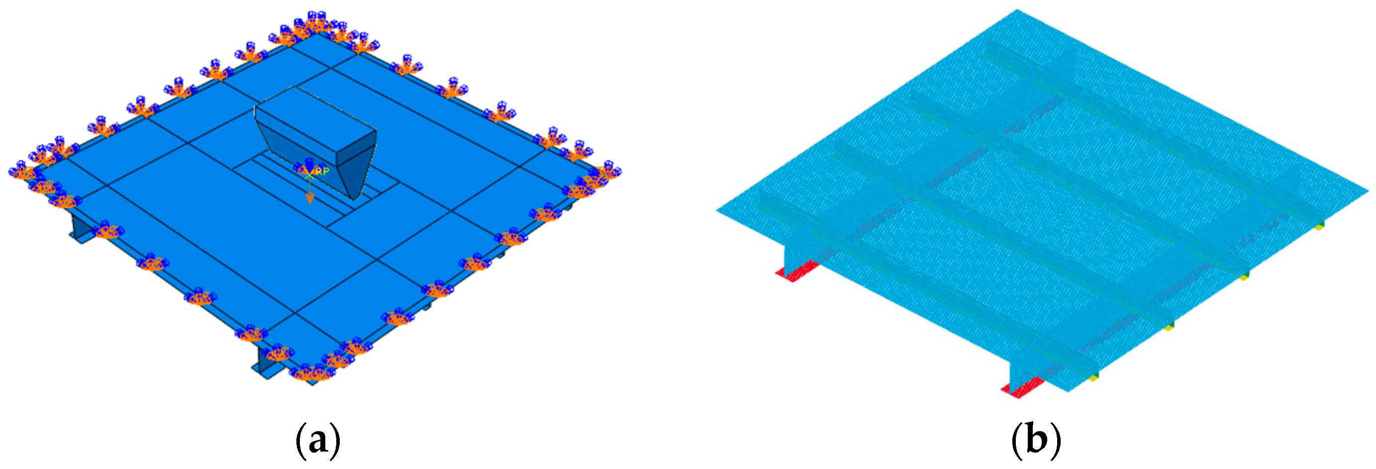
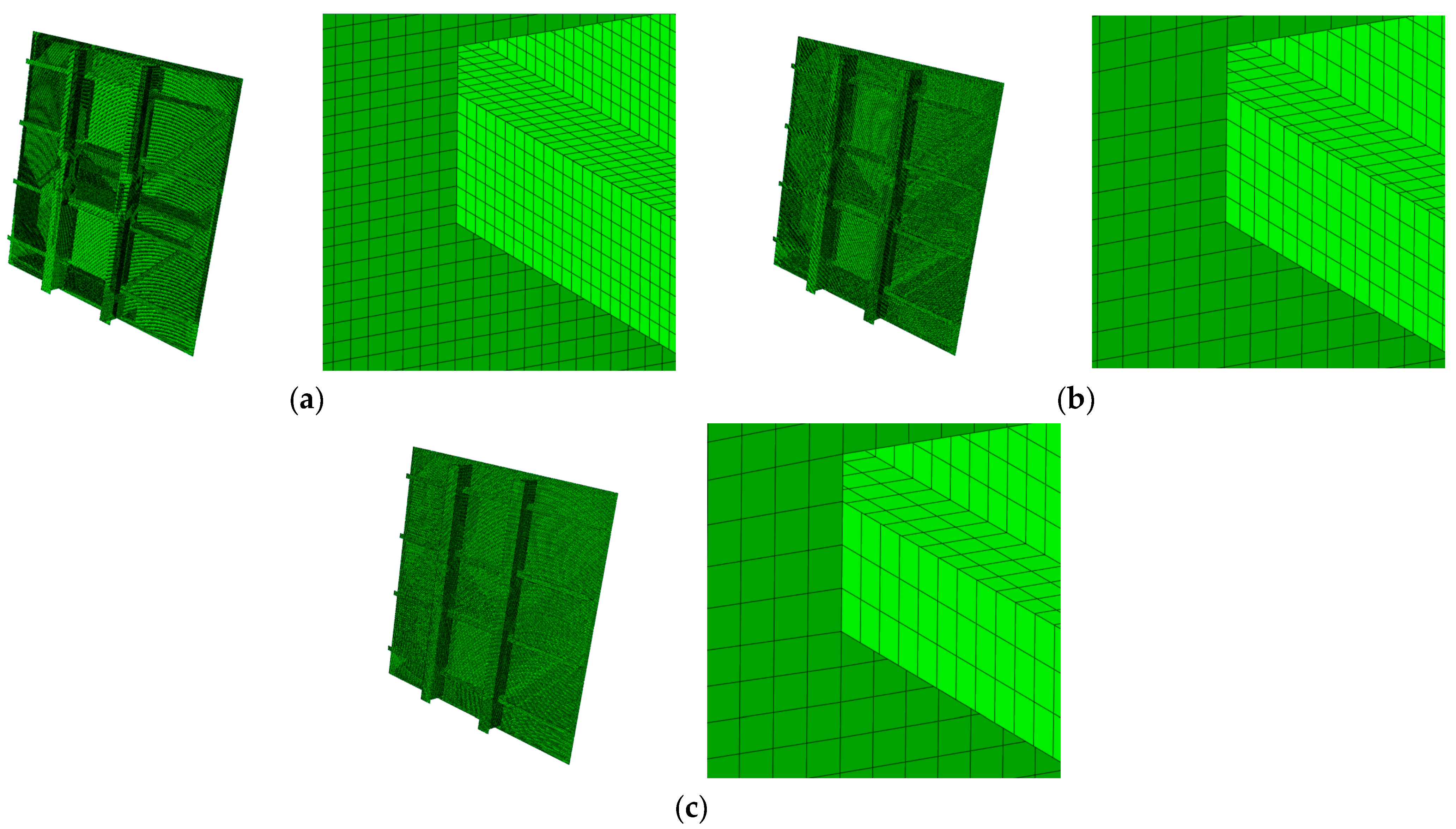
3.3. Finite Element Model
3.4. Comparison of Simulation and Test Results
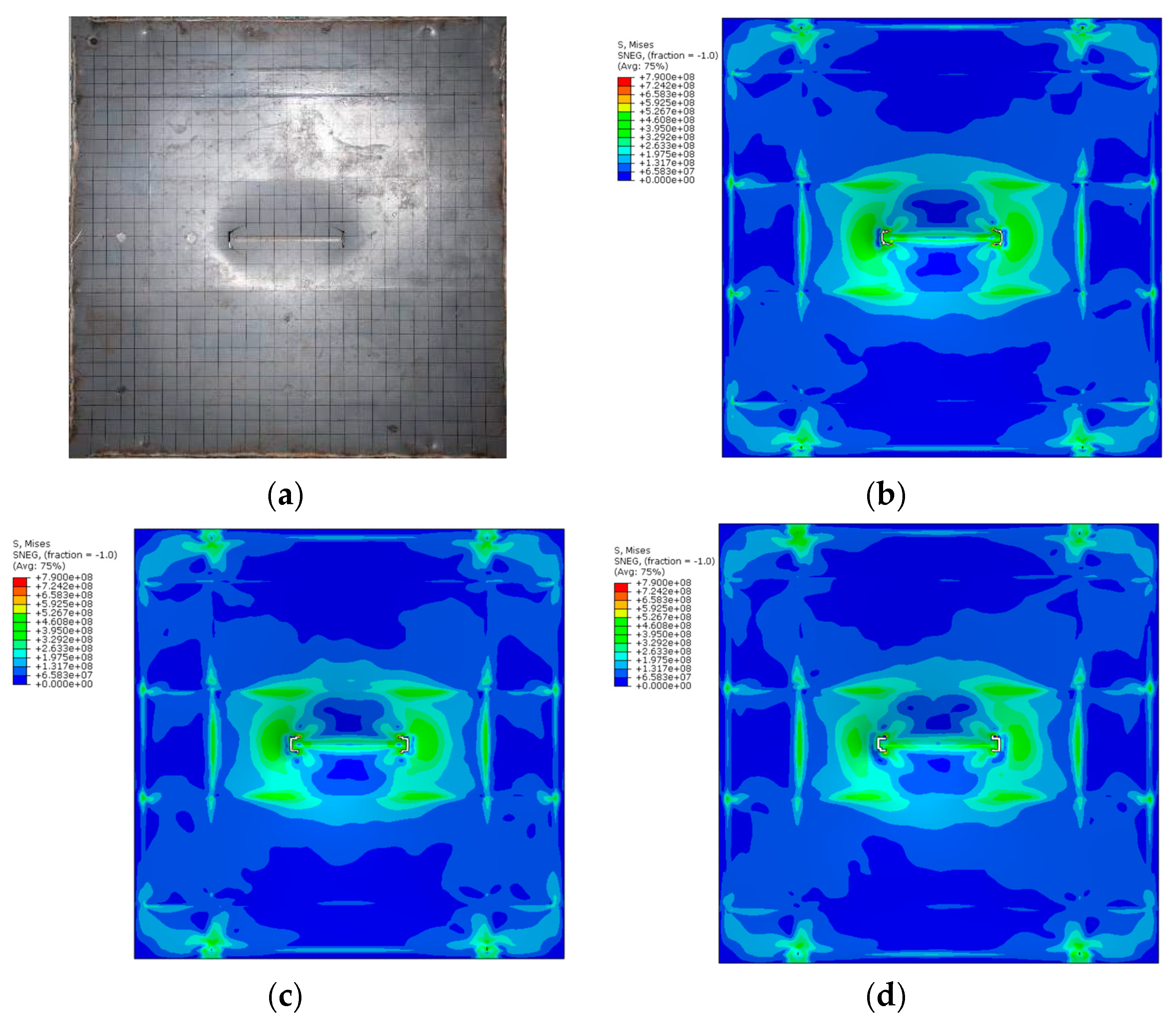
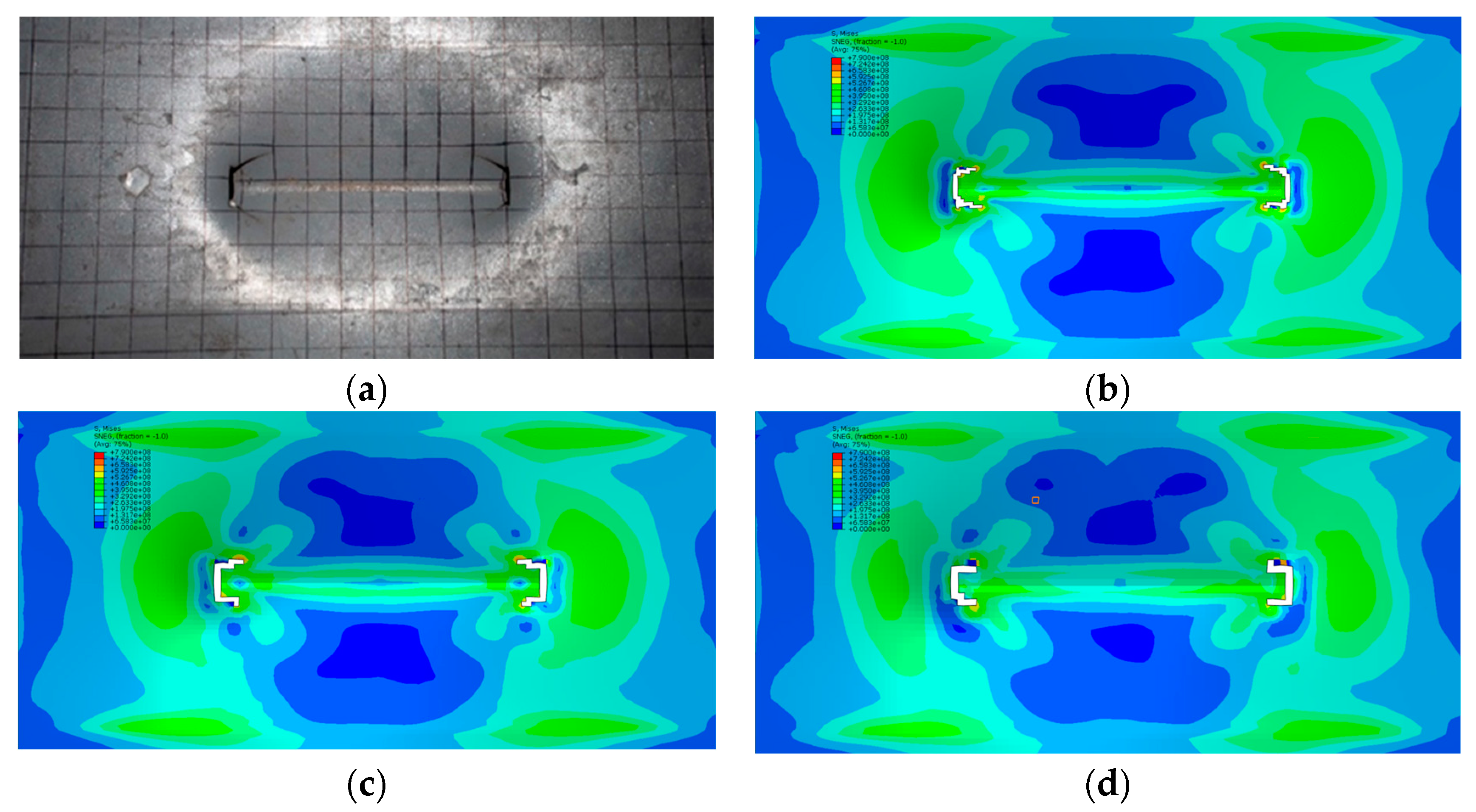
3.4.1. Damage Deformation
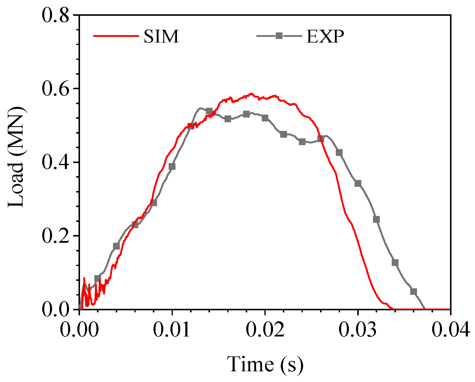
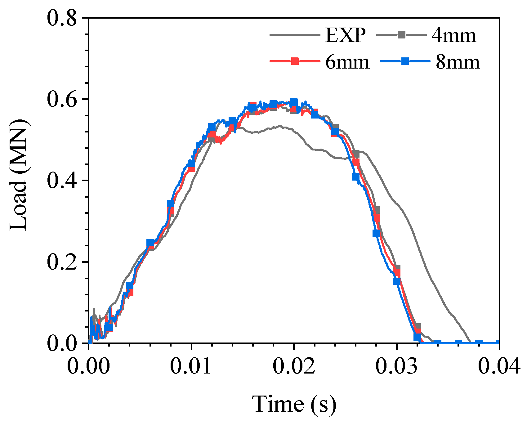
3.4.2. Force–Time Curve of Collision
4. Discussion
4.1. Common Fracture Failure Criteria in Ship Collision Simulation
4.1.1. Equivalent Plastic Strain Criterion
4.1.2. RTCL Failure Criterion
4.2. Comparative Analysis of Impact Responses of Stiffened Panels under Drop-Weight Collisions Using Different Failure Criteria
4.3. Mesh Size Sensitivity Study of the MMC Failure Criterion
5. Conclusions
Author Contributions
Funding
Institutional Review Board Statement
Informed Consent Statement
Data Availability Statement
Conflicts of Interest
References
- Alsos, H.; Hopperstad, O.; Törnqvist, R.; Amdahl, J. Analytical and numerical analysis of sheet metal instability using a stress based criterion. Int. J. Solids Struct. 2008, 45, 2042–2055. [Google Scholar] [CrossRef]
- Hill, R. On discontinuous plastic states, with special reference to localized necking in thin sheets. J. Mech. Phys. Solids 1952, 1, 19–30. [Google Scholar] [CrossRef]
- Minorsky, V. An Analysis of Ship Collisions with Reference to Protection of Nuclear Power Plants; Sharp (George G.) Inc.: New York, NY, USA, 1958. [Google Scholar]
- Haris, S.; Amdahl, J. Analysis of ship–ship collision damage accounting for bow and side deformation interaction. Mar. Struct. 2013, 32, 18–48. [Google Scholar] [CrossRef]
- Törnqvist, R. Design of Crashworthy Ship Structures; Technical University of Denmark: Kongens Lyngby, Denmark, 2003. [Google Scholar]
- Ehlers, S.; Broekhuijsen, J.; Alsos, H.S.; Biehl, F. Simulating the collision response of ship side structures: A failure criteria benchmark study. Int. Shipbuild. Prog. 2008, 55, 127–144. [Google Scholar] [CrossRef]
- Storheimabe, M.; Amdahl, J.; Martens, I. On the accuracy of fracture estimation in collision analysis of ship and offshore structures. Mar. Struct. 2015, 44, 254–287. [Google Scholar] [CrossRef]
- Driemeier, L.; Brünig, M.; Micheli, G.; Alves, M. Experiments on stress-triaxiality dependence of material behavior of aluminum alloys. Mech. Mater. 2010, 42, 207–217. [Google Scholar] [CrossRef]
- Wang, Z.; Hu, Z.; Liu, K.; Chen, G. Application of a material model based on the Johnson-Cook and Gurson-Tvergaard-Needleman model in ship collision and grounding simulations. Ocean Eng. 2020, 205, 106768. [Google Scholar] [CrossRef]
- Calle, M.A.G.; Alves, M. A review-analysis on material failure modeling in ship collision. Ocean Eng. 2015, 106, 20–38. [Google Scholar] [CrossRef]
- Bai, Y.; Wierzbicki, T. Application of extended Mohr–Coulomb criterion to ductile fracture. Int. J. Fract. 2009, 161, 1–20. [Google Scholar] [CrossRef]
- Lou, Y.; Huh, H. Evaluation of ductile fracture criteria in a general three-dimensional stress state considering the stress triaxiality and the lode parameter. Acta Mech. Solida Sin. 2013, 26, 642–658. [Google Scholar] [CrossRef]
- Hu, Q.; Li, X.; Han, X.; Chen, J. A new shear and tension based ductile fracture criterion: Modeling and validation. Eur. J. Mech. A/Solids 2017, 66, 370–386. [Google Scholar] [CrossRef]
- Bao, Y.; Wierzbicki, T. On fracture locus in the equivalent strain and stress triaxiality space. Int. J. Mech. Sci. 2004, 46, 81–98. [Google Scholar] [CrossRef]
- Talebi-Ghadikolaee1, H.; Naeini1, H.; Mirnia, M.; Mirzai, M.; Alexandrov, S.; Gorji, H. Experimental and numerical investigation of failure during bending of AA6061 aluminum alloy sheet using the modified Mohr-Coulomb fracture criterion. Int. J. Adv. Manuf. Technol. 2019, 105, 5217–5237. [Google Scholar] [CrossRef]
- Voormeeren, L.; Walters, C.; Tang, L.; Vredeveldt, A. Estimation of failure parameters for finite element simulations based on a single state of stress and arbitrary stress-strain relation. In Proceedings of the ASME 2014 33rd International Conference on Ocean, Offshore and Arctic Engineering OMAE 2014, San Francisco, CA, USA, 8–13 June 2014. [Google Scholar]
- Zhu, L.; Estefen, S.; Lourenço, M. Fracture criteria applied to numerical simulation of blowout preventer ram shearing. Eng. Fail. Anal. 2020, 114, 104596. [Google Scholar] [CrossRef]
- Mohr, O. Abhandlungen Aus Dem Gebiete Der Technischen Mechanik; W. Ernst & Sohn: Berlin, Germany, 1914. [Google Scholar]
- Bao, Y.; Wierzbicki, T. A comparative study on various ductile crack formation criteria. J. Eng. Mater. Technol. 2004, 126, 314–324. [Google Scholar] [CrossRef]
- Yu, R.; Li, X.; Yue, Z.; Li, A.; Zhao, Z.; Wang, X.; Zhou, H.; Lu, T.J. Stress state sensitivity for plastic flow and ductile fracture of L907A low-alloy marine steel: From tension to shear. Mater. Sci. Eng. A 2022, 835, 142689. [Google Scholar] [CrossRef]
- Dassault Sastemes. SIMULIA User Assistance 2020. Available online: https://help.3ds.com/2020/english/dssimulia_established/SIMACAESUBRefMap/simasub-c-vumat.htm?contextscope=all (accessed on 4 April 2024).
- Ling, Y. Uniaxial true stress-strain after necking. AMP J. Technol. 1996, 5. [Google Scholar]
- Liu, H.; Liu, K.; Wang, X.; Gao, Z.; Wang, J. On the Resistance of Cruciform Structures during Ship Collision and Grounding. J. Mar. Sci. Eng. 2023, 11, 459. [Google Scholar] [CrossRef]
- Liu, K.; Zong, S.; Li, Y.; Wang, Z.; Hu, Z.; Wang, Z. Structural response of the U-type corrugated core sandwich panel used in ship structures under the lateral quasi-static compression load. Mar. Struct. 2022, 84, 103198. [Google Scholar] [CrossRef]
- Liu, K.; Liu, H.; Li, Y.; Wang, Z.; Wang, J. A Simplified Method for Evaluating the Dynamic Response of the Metal Sandwich Structure under Explosion Load. Metals 2022, 12, 1933. [Google Scholar] [CrossRef]
- Rice, J.R.; Tracey, D.M. On the ductile enlargement of voids in triaxial stress fields. J. Mech. Phys. Solids 1969, 17, 201–217. [Google Scholar] [CrossRef]
- Cockcroft, M. Ductility and workability of metals. J. Met. 1968, 96, 2444. [Google Scholar]
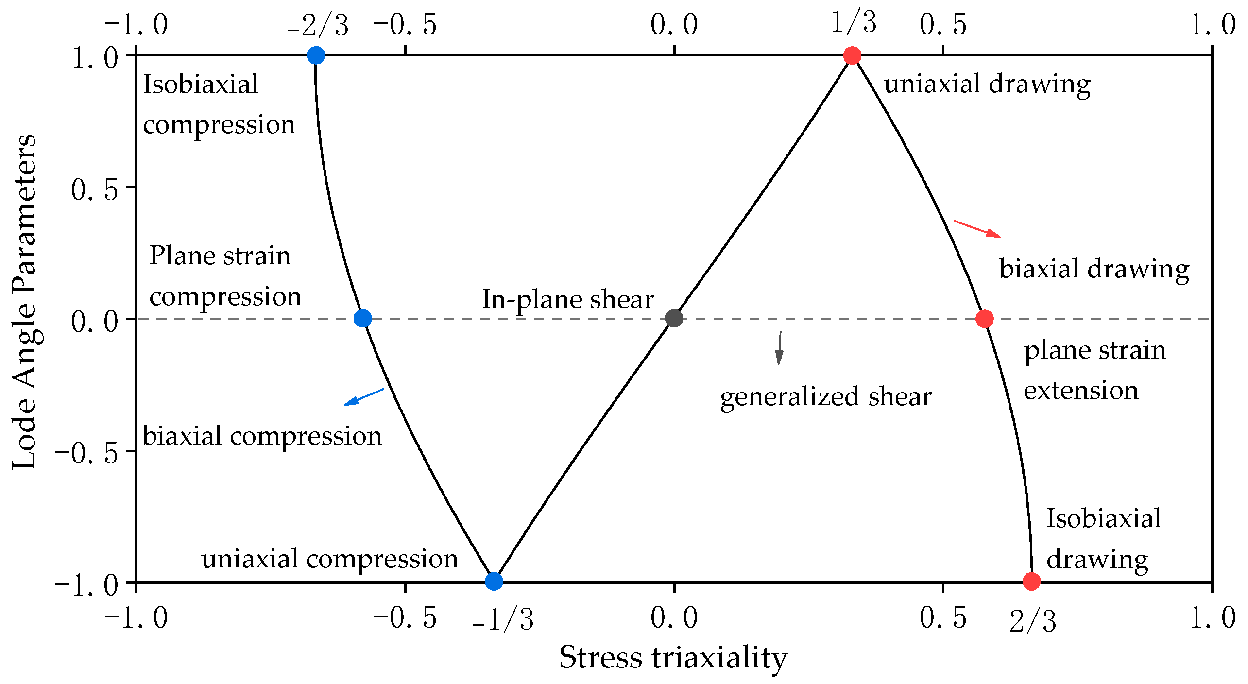
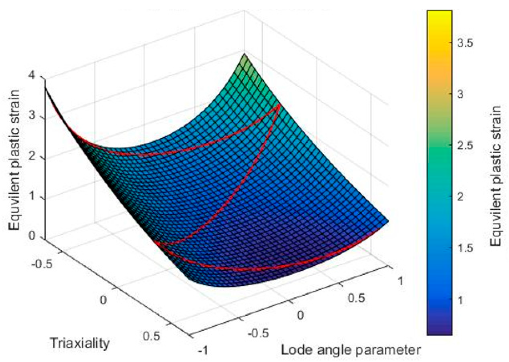


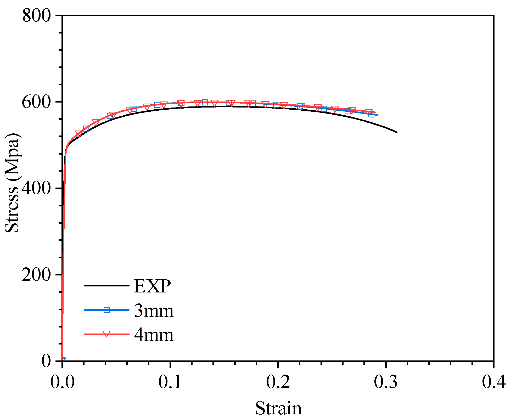
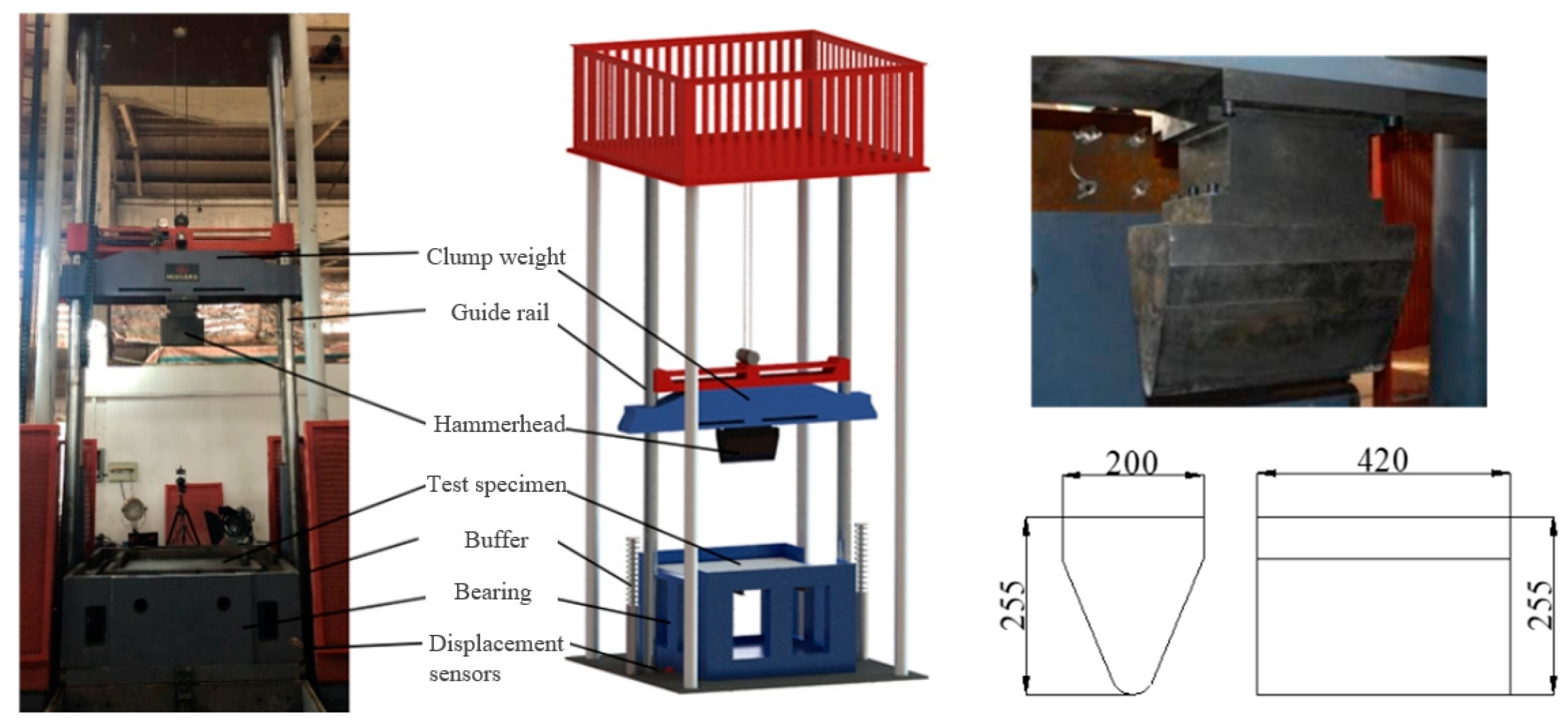







| Sample Type | Specimen Number | |||
|---|---|---|---|---|
| Notched round bar | NRB6 | 0.443 | 1 | 1.091 |
| NRB1.5 | 0.716 | 1 | 0.910 | |
| Grooved plate | FGP12 | 0.593 | 0 | 0.905 |
| FGP1.8 | 0.765 | 0 | 0.830 | |
| Notched plate | NP20 | 0.446 | 0.614 | 1.018 |
| NP6.67 | 0.554 | 0.213 | 0.973 | |
| Shear | SH | −0.037 | 0.024 | 0.859 |
| K | N | c1 | c2 |
|---|---|---|---|
| 909.29 MPa | 0.1992 | 0.0420 | 301.47 MPa |
| Density ρkg/m3 | Elastic Modulus E Gpa | Poisson Ratio | Yield Stress Mpa | Failure Strain |
|---|---|---|---|---|
| 7850 | 210 | 0.3 | 470 | 0.28 |
| Specimen Name | Quilting Material Spacing | Falling Weight Height | Slab Dimension | Bone Size | Bone Spacing | Truss Size |
|---|---|---|---|---|---|---|
| Plate frame structure | 1000 | 2000 | 1560 × 1560 × 4 | 6# bulb flat | 390 |
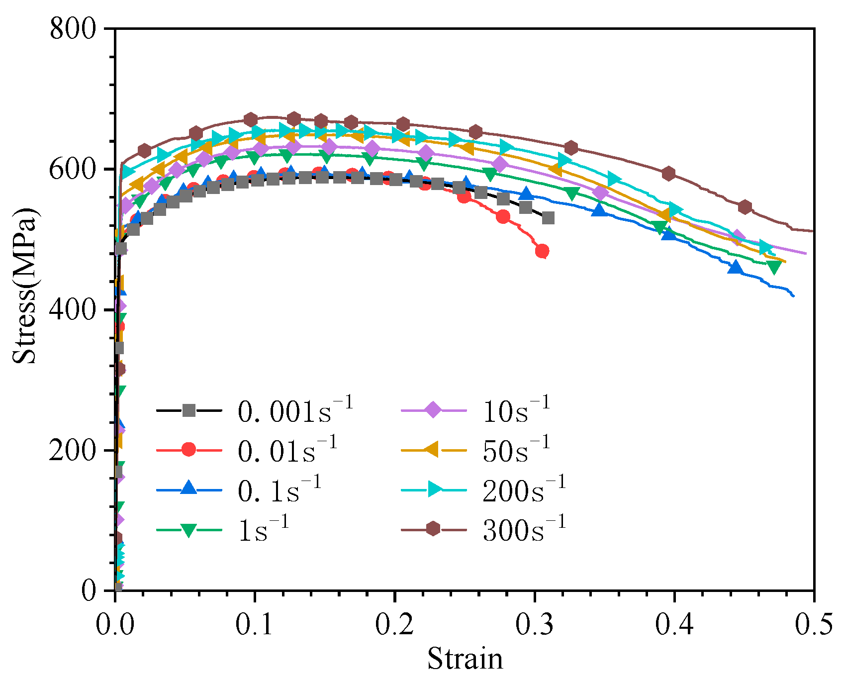
| strain rate/s−1 | 0.001 | 0.01 | 0.1 | 1 | 10 | 50 | 200 | 300 |
| yield stress/MPa | 489 | 501 | 516 | 540 | 541 | 561 | 592 | 608 |
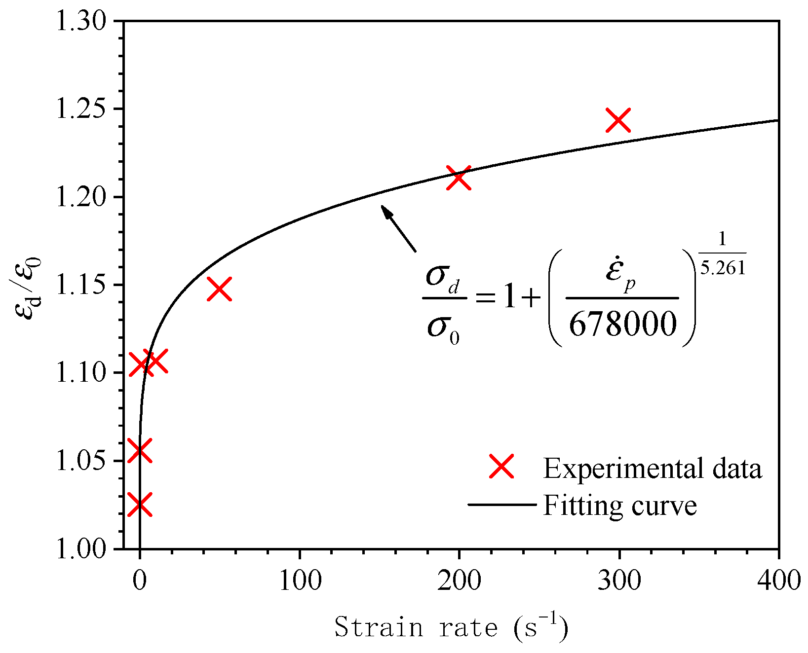
| Density ρkg/m3 | Elastic Modulus E Gpa | Poisson Ratio | Yield Stress Mpa | Failure Strain | D | q |
|---|---|---|---|---|---|---|
| 7850 | 210 | 0.3 | 470 | 0.28 | 678,000 | 5.261 |
| Failure Criterion | Collision Force Peak (MN) | Error (%) |
|---|---|---|
| EXP | 0.547 | 0 |
| MMC | 0.5854 | 7.02 |
| RTCL | 0.6004 | 9.76 |
| EPS | 0.6426 | 17.48 |
| Failure Criterion | Collision Energy (KJ) | Error (%) |
|---|---|---|
| EXP | 22.51 | 0 |
| MMC | 22.51 | 0.02 |
| RTCL | 22.46 | 0.20 |
| EPS | 22.03 | 2.11 |
Disclaimer/Publisher’s Note: The statements, opinions and data contained in all publications are solely those of the individual author(s) and contributor(s) and not of MDPI and/or the editor(s). MDPI and/or the editor(s) disclaim responsibility for any injury to people or property resulting from any ideas, methods, instructions or products referred to in the content. |
© 2024 by the authors. Licensee MDPI, Basel, Switzerland. This article is an open access article distributed under the terms and conditions of the Creative Commons Attribution (CC BY) license (https://creativecommons.org/licenses/by/4.0/).
Share and Cite
Liu, S.; Liu, K.; Liu, H.; Zong, S.; Lu, Y.; Liu, C. Calibration of the Modified Mohr–Coulomb Failure Criterion and Its Application in the Study of Collision Response of Ship Hull Plate Frame Structures. J. Mar. Sci. Eng. 2024, 12, 805. https://doi.org/10.3390/jmse12050805
Liu S, Liu K, Liu H, Zong S, Lu Y, Liu C. Calibration of the Modified Mohr–Coulomb Failure Criterion and Its Application in the Study of Collision Response of Ship Hull Plate Frame Structures. Journal of Marine Science and Engineering. 2024; 12(5):805. https://doi.org/10.3390/jmse12050805
Chicago/Turabian StyleLiu, Shiye, Kun Liu, Hewei Liu, Shuai Zong, Yue Lu, and Chuhao Liu. 2024. "Calibration of the Modified Mohr–Coulomb Failure Criterion and Its Application in the Study of Collision Response of Ship Hull Plate Frame Structures" Journal of Marine Science and Engineering 12, no. 5: 805. https://doi.org/10.3390/jmse12050805
APA StyleLiu, S., Liu, K., Liu, H., Zong, S., Lu, Y., & Liu, C. (2024). Calibration of the Modified Mohr–Coulomb Failure Criterion and Its Application in the Study of Collision Response of Ship Hull Plate Frame Structures. Journal of Marine Science and Engineering, 12(5), 805. https://doi.org/10.3390/jmse12050805


