Article

Development and Use of Tide Models in Alaska Supporting VDatum and Hydrographic Surveying

1
Coast Survey Development Laboratory, National Ocean Service, National Oceanic and Atmospheric Administration, 1315 East-West Highway, Silver Spring, MD 20910, USA
2
Earth Resources Technology, Inc., 14401 Sweitzer Lane, Suite 300, Laurel, MD 20707, USA
3
Center for Operational Oceanographic Products and Services, National Ocean Service, National Oceanic and Atmospheric Administration, 1305 East-West Highway, Silver Spring, MD 20910, USA
4
The Baldwin Group, 8573-D Sudley Road, Manassas, VA 20110, USA
*
Author to whom correspondence should be addressed.
J. Mar. Sci. Eng. 2014, 2(1), 171-193; https://doi.org/10.3390/jmse2010171
Submission received: 29 November 2013 / Revised: 25 January 2014 / Accepted: 8 February 2014 / Published: 10 March 2014

Abstract

:
National Oceanic and Atmospheric Administration’s National Ocean Service uses observations, hydrodynamic models and interpolation techniques to develop many of its products and services. We examine how two projects, computation of tidal datums for vertical datum transformation and the estimation of tidal characteristics for hydrographic surveys, are being developed in Alaska and how they may be more seamlessly integrated. Preliminary VDatum development for Alaska is in progress for the Alaska Panhandle through the setup of a high resolution tide model that will be used to compute spatially varying tidal datums. Tide models such as these can be used for other projects that traditionally rely on estimation of tides in between data locations, such as the planning for hydrographic surveys that need correctors to adjust bathymetry to the chart datum. We therefore also examine how an existing model in western Alaska can be used for better supporting hydrographic survey planning. The results show that integration of tide models with nearshore observations can provide improved information for these correctors and future work will further evaluate this methodology with existing VDatum tide models.

1. Introduction

National Oceanic and Atmospheric Administration (NOAA)’s National Ocean Service (NOS) develops and uses tide models and interpolation techniques in support of vertical datum transformation and hydrographic surveying. In this paper, we describe initial efforts to expand these capabilities in Alaska. VDatum [1] is a vertical datum transformation software tool, and the tidal datum transformations in VDatum are normally computed by using tide model results and corrected by interpolation [2]. These tidal datums are then related to orthometric and ellipsoid-based vertical reference systems through geoid models developed by NOS’ National Geodetic Survey (NGS). Developing VDatum for Alaska presents many challenges, mainly due to the smaller amount of tidal, orthometric and GPS data available to support the development and validation of models used to generate the vertical datums and their relationships to each other. While more of the data is being collected, the VDatum team decided that the development of a tide model could begin in one selected subregion of Alaska, using existing tide data to help validate the model. As more data becomes available in the future, any necessary adjustments to the model to improve model-observation agreement could be made accordingly. Additionally, tide models developed for VDatum are increasingly being used to help address other needs within NOAA. An example of this is hydrographic survey planning, where tidal parameters normally estimated through interpolation of tide gauge data could benefit from modeled tidal characteristics between gauge locations. While development of the identified subregional tide model is in progress, we also evaluated how an existing tide model could be used to better define the spatial variability of tidal parameters to support hydrographic planning in western Alaska.
VDatum tidal datums are normally developed by first simulating tidal characteristics with the advanced circulation model (ADCIRC) [3,4]. The VDatum team evaluated: (1) how to break the Alaska region into subregions; and (2) which subregion would have the highest priority for tide model development. We decided that at least five subregions would be needed and, based partially on the feedback from VDatum users, that southeast (SE) Alaska is the best suited for initial development (Figure 1a,b). Several tidal model applications have been previously developed covering SE Alaska [5,6,7,8,9]. Most of these applications emphasize regional tidal propagation, with a minimum resolution near the coast sufficient to resolve major passages and waterways around the Alexander Archipelago [5,6,7]. Hill et al. [8] simulated the tides and fresh water runoff in Glacier Bay, Alaska, using ADCIRC with a high resolution unstructured grid. Inazu et al. [9] modeled tides in SE Alaska using a finite difference model with 1-km resolution and gave an estimation of large tidal dissipation around Glacier Bay. There are also Pacific basin scale and global scale tidal models available, notably the Oregon State University Tidal Inversion Software (OTIS) by Egbert and Erofeeva [10,11] and the last version of the FES (Finite Element Solution) global tide model developed in 2012, FES2012 [12]. OTIS project has a Pacific basin scale model at 1/12° resolution, PO2009, as well as a global model, TPXO7.2, that assimilates satellite altimetry data. The diurnal and semidiurnal tides in the Gulf of Alaska from these models all have similar spatial patterns [5,6,7,10,11,12]. While the overall offshore pattern is simple, the complexity of the passages and waterways inside the SE Alaska Panhandle leads to significant tidal wave deflection and dissipation and thus requires a high resolution tidal model to properly simulate the local tidal propagation and spatial variations in tidal datums [13]. Therefore, initial work towards a new tide model for SE Alaska is presented here with higher resolution to resolve both regional and local tidal dynamics.
Figure 1. (a) Alaska shoreline and coast waters, and the southeast (SE) Alaska hydrodynamic model domain (blue polygon, approximately); (b) SE Alaska, bathymetry and tidal stations (green dots); (c) SE Alaska unstructured model grid.
Jmse 02 00171 g001
With the start of work on the SE Alaska tide model for eventual VDatum development, the VDatum team is also looking at extending the use of tide models developed over the years for VDatum along the U.S. coasts. One such identified use is to provide offshore tidal constituents to NOAA’s Hydrographic Planning Team (HPT) in the Center for Operational Oceanographic Products and Services (CO-OPS). In the assessment of users’ needs in Alaska for VDatum and tide models, HPT was identified for collaboration on evaluating the use of tide model outputs as an additional source of information to support hydrographic surveys in the Bering Sea. HPT provides survey operation teams with estimated tidal curves within a survey area by interpolating/extrapolating tidal constituents and tidal parameters, such as the mean tidal range (MN) and the high water interval (HWI, the interval between the Moon’s transit over the Greenwich meridian and the following high water). Current interpolation/extrapolation relies on the constituents and parameters derived from CO-OPS’ measurements at tide gauges located along the shoreline. The tidal constituents and tidal parameters derived from model results should therefore provide better estimates for offshore tides. The Bering Sea of western Alaska has complex tidal characteristics with several diurnal and semidiurnal amphidromes. Some previous tide models [14,15] are able to capture large-scale tidal features, but tend to perform worse in the nearshore regions, due to their relatively coarse resolution. Foreman et al. [16] used a variable triangular grid with a resolution from 1.5 km to 50 km and a barotropic finite element model to simulate tides in the Bering Sea with the assimilation of tidal harmonics derived from satellite altimetry data. Foreman's model has relatively high accuracy in the offshore and nearshore regions (the average M2 root mean square error, RMSE, is 3.0 cm; see Section 3.3 for details), even though it is less accurate at the onshore CO-OPS tide stations (the average M2 RMSE is 10.7 cm; see Section 3.2 for details). We therefore used Foreman’s model for evaluation in this study and present the results of incorporating the model results into estimated tidal patterns to help support hydrographic survey planning. We will refer to Foreman’s model as “FM” in all future discussion.
This paper is organized as follows: Section 2 presents the work on the development of a new, high-resolution tidal model for SE Alaska. Section 3 evaluates how tide models can improve current methods of estimating offshore tidal patterns to provide tide correctors for hydrographic surveys. The development of new tide models for the remainder of Alaska and further analysis of the use of tide models in hydrographic planning will continue in future years, and Section 4 identifies some key objectives of future work in this regard.

2. Tidal Modeling in SE Alaska

As the first step towards VDatum availability in southeast Alaska, the development of a high resolution ADCIRC tidal model is presented here for the coastal waters around the Alexander Archipelago and Alaska Panhandle. Using high-resolution shoreline and bathymetric data from NOAA, this model is able to resolve the fine detail of the shoreline with resolution down to about 50 m. Boundary conditions were obtained from Oregon State University’s regional tidal solution PO2009 tide database [17] for the M2, S2, N2, K2, K1, O1, P1, Q1, M4, MS4 and MN4 constituents. The skill of the model is assessed through comparison of amplitudes and phases of tidal constituents derived from the model and from observations. After model validation, the model will be used to compute tidal datums for future use in NOAA’s VDatum software.

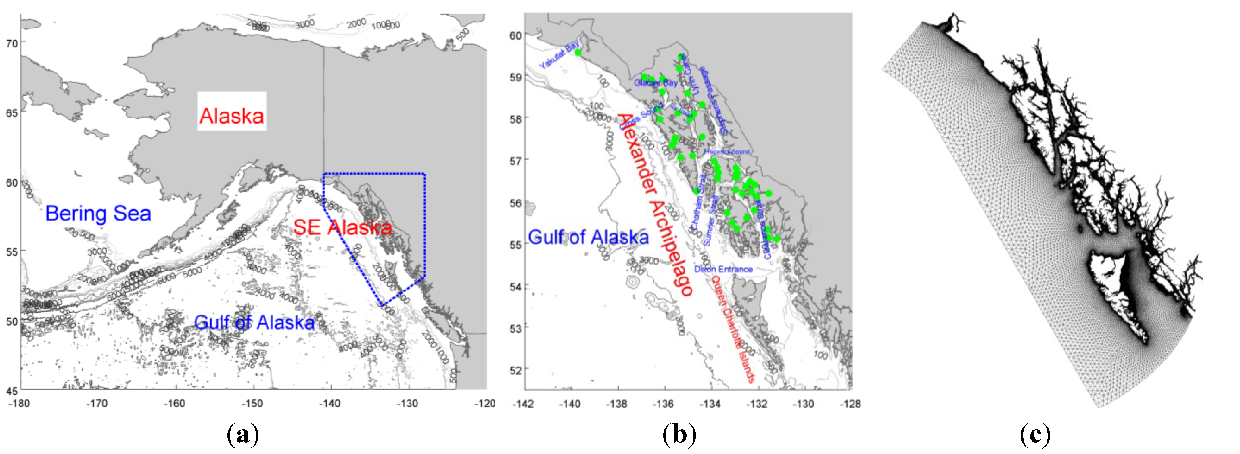
2.1. Model Development

The model domain covers all coastal waters of the SE Alaska Panhandle (Figure 1). To reduce the impact of errors propagated from the open ocean boundary, we extend the southern open boundary beyond the southern tip of the Queen Charlotte Islands and the northern open boundary to include Yakutat Bay. The length of the domain from south to north is about 1150 km. In the offshore direction, the open boundary is extended to about 200 km from the nearest islands. The entire water domain covers a total of 300,000 km2. For regions inside the U.S. marine boundary, two types of bathymetric data were used: (1) sounding data of individual depth measurements; and (2) a digital elevation model (DEM) composed of multiple data sources [18]. For regions further offshore, a one arc-minute global relief model, ETOPO1 [19] was used. The reference vertical datums of the sounding data and DEM were converted to mean sea level (MSL) using gridded vertical datum conversions provided by NOAA’s National Geophysical Data Center (NGDC). These conversions were calculated using kriging to interpolate the vertical datums from 93 tide gauges around SE Alaska [20]. The vertical datum of ETOPO1 is mean sea level and therefore did not require a datum conversion. The bathymetry was smoothed to reduce the maximum slope and prevent instabilities, due to steep bottom slopes. A mean high water shoreline dataset was provided by NOAA’s NGS.
An unstructured triangular mesh grid (Figure 1c) was generated to represent the model domain, using the shoreline from NGS as the land boundary. The water depths, distance to the shoreline and desired minimum resolution along the shoreline were among the factors used for determining local mesh resolution. The current mesh grid has about two million node points. The smallest grid size is 50 m and the largest is about 20 km. Bathymetry was interpolated to the model grid using linear interpolation.
A state-of-the-art numerical hydrodynamic model, ADCIRC [3,4], was used for tidal simulations with the SE Alaska grid. ADCIRC solves the 2D vertically-integrated generalized wave continuity equation using the finite element method on an unstructured triangular grid. This model has been widely applied to tide and storm surge simulations in estuarine, coastal and continental shelf regions [21].
To properly set up the model, three boundary conditions have to be prescribed: open boundary, surface boundary and bottom boundary conditions. Since we are only simulating the tides, there is no air-sea exchange of momentum, mass and energy applied to the surface boundary. A slip quadratic bottom friction boundary condition is used for the bottom boundary. We use a depth-dependent bottom friction coefficient, Cf,
Jmse 02 00171 i001
where z is water depth, Hs and Hd are two constant water depths, equal to 100 m and 300 m, respectively, in this study, and Jmse 02 00171 i002 and Jmse 02 00171 i003 are constant bottom friction coefficients for water shallower than Hs and water deeper than Hd, respectively. Equation 1 provides a depth-dependent linear interpolated bottom friction for water depths between Hs and Hd. In this study, we use Cf = Cf (0.00375,0.00375), a constant over all depths, for the baseline study, and variable Cf scenarios are examined in sensitivity tests. The open boundary is forced by prescribed tidal information interpolated from Oregon State University’s Pacific Ocean basin scale tidal solution PO2009 [17]. The tidal forcing along the open boundary consisted of four semidiurnal constituents (M2, S2, N2 and K2), four diurnal constituents (K1, O1, P1 and Q1) and three shallow water components (M4, MS4 and MN4). The model has wetting and drying enabled, so as to cope with tidal flat scenarios.

2.2. Model Validation

Tidal harmonic constants for these 11 constituents (M2, S2, N2, K2, K1, O1, P1, Q1, M4, MS4 and MN4) are used for model validation at 43 CO-OPS tidal stations (Figure 1b). Some of these stations are long-term, active stations, while others are historical stations with various time lengths of deployment [22].
The semidiurnal M2 tide in the Gulf of Alaska has an amphidrome in the northern Pacific Ocean, east of Hawaii. The M2 tide propagates anticlockwise along the coast of SE Alaska, with the co-phase lines perpendicular to the coast and co-amplitude lines parallel to the coast (Figure 2). There are many inter-island waterways and passages along the SE Alaska coast through which the tides branch out and propagate shoreward. Some of these major passages include the Dixon Entrance-Clearance Strait, Sumner Strait, Chatham Strait and Cross Sound in the north (Figure 1b). Once inside the passages, the tide propagates through waterways with increasing phase lag and generally increasing amplitude. The amplitude near the open boundary is about 1 m. There are locations at the ends of inlets and passages, notably in Glacier Bay, Lynn Canal and Stephens Passage, where the amplitude is larger than 2 m (Figure 2). Glacier Bay has some of the largest amplitudes and phase lags in the model domain.
Figure 2. M2 tide (a) co-amplitude lines (meters); and (b) co-phase lines (degrees) in SE Alaska.
Jmse 02 00171 g002
The diurnal tide, K1, in the Gulf of Alaska has an amphidrome in the northern Pacific Ocean, west of Hawaii. The K1 tide propagates anticlockwise in the northwest direction along the SE Alaska coast. The amplitude of K1 near the open boundary is about 0.45 m and increases landwards (Figure 3). The maximum K1 amplitude in Glacier Bay is around 0.6 m. Similar to the M2 tide, the K1 phase lag increases in the northwest direction, but with less of a phase lag gradient. The largest phase lag is in Glacier Bay, around 270 degrees. In comparison, at the southern tip of the Alexander Archipelago, just north of the Dixon entrance, the K1 phase is about 258 degrees. All other semidiurnal and diurnal tides had similar patterns as the dominant M2 and K1 tides, only with smaller amplitudes.
A direct comparison between model and observed M2 amplitudes (Figure 4) shows that the model generally overestimates the M2 amplitude. The amplitude (observed, model) pairs are clustered along the 5% error line. The model underestimates M2 amplitudes only at two stations and overestimates more than 10% at one station. The M2 phase is generally underestimated. At the lower phase values (i.e., at locations closer to the southern open boundary), this underestimation is smaller. This can be due to the accumulation of error with the phase along the direction of wave propagation. For the S2 tide, the results are similar. For the K1 and O1 tides, the model overestimates the amplitude and underestimates the phase. The difference in both amplitude and phase is more of a constant shift. This may suggest that applying a constant shift to the K1 and O1 boundary conditions could help improve the results.
Figure 3. K1 tide (a) co-amplitude lines (meters); and (b) co-phase lines (degrees) in SE Alaska.
Jmse 02 00171 g003
Figure 4. M2, S2, K1 and O1 model-observation comparison of amplitude (meters) and phase (degrees) at 43 tidal stations in SE Alaska.
Jmse 02 00171 g004
To quantify the model performance and skill, we calculated the mean absolute error (MAE) of the amplitudes and phases. We also calculated the root mean square error (RMSE), Ae, which combines the amplitude error and phase error using the equation:
Jmse 02 00171 i004
where Ao and Am are observed and modeled amplitudes, respectively, and ho and hm are observed and modeled phases, respectively. The relative RMSE (%), Jmse 02 00171 i005
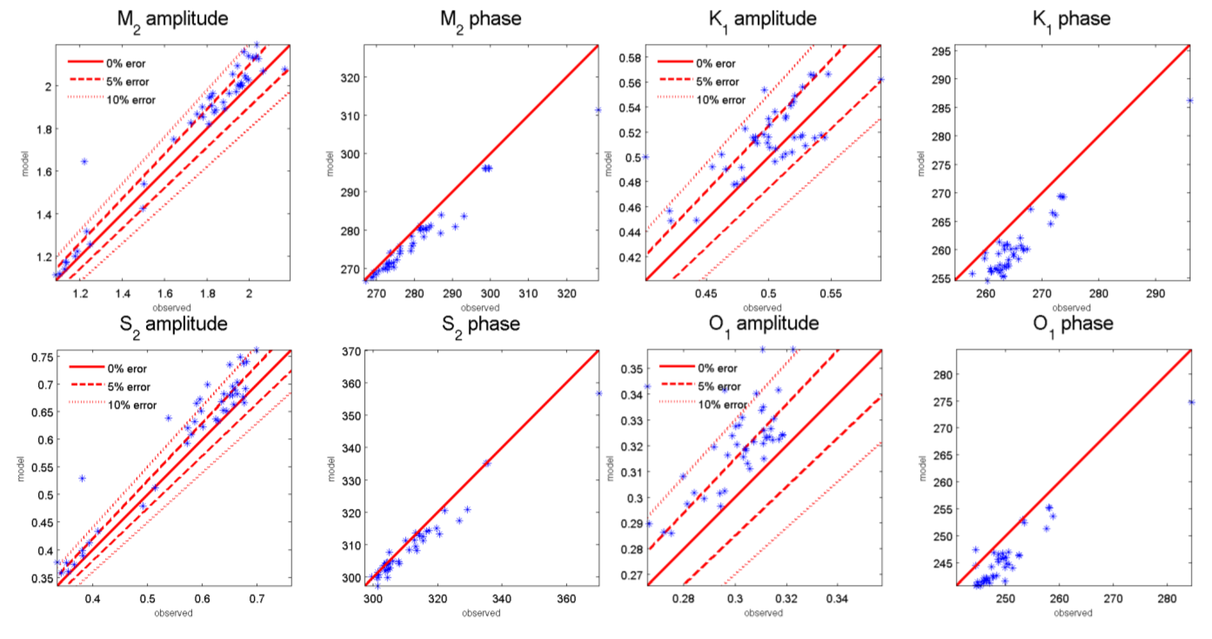
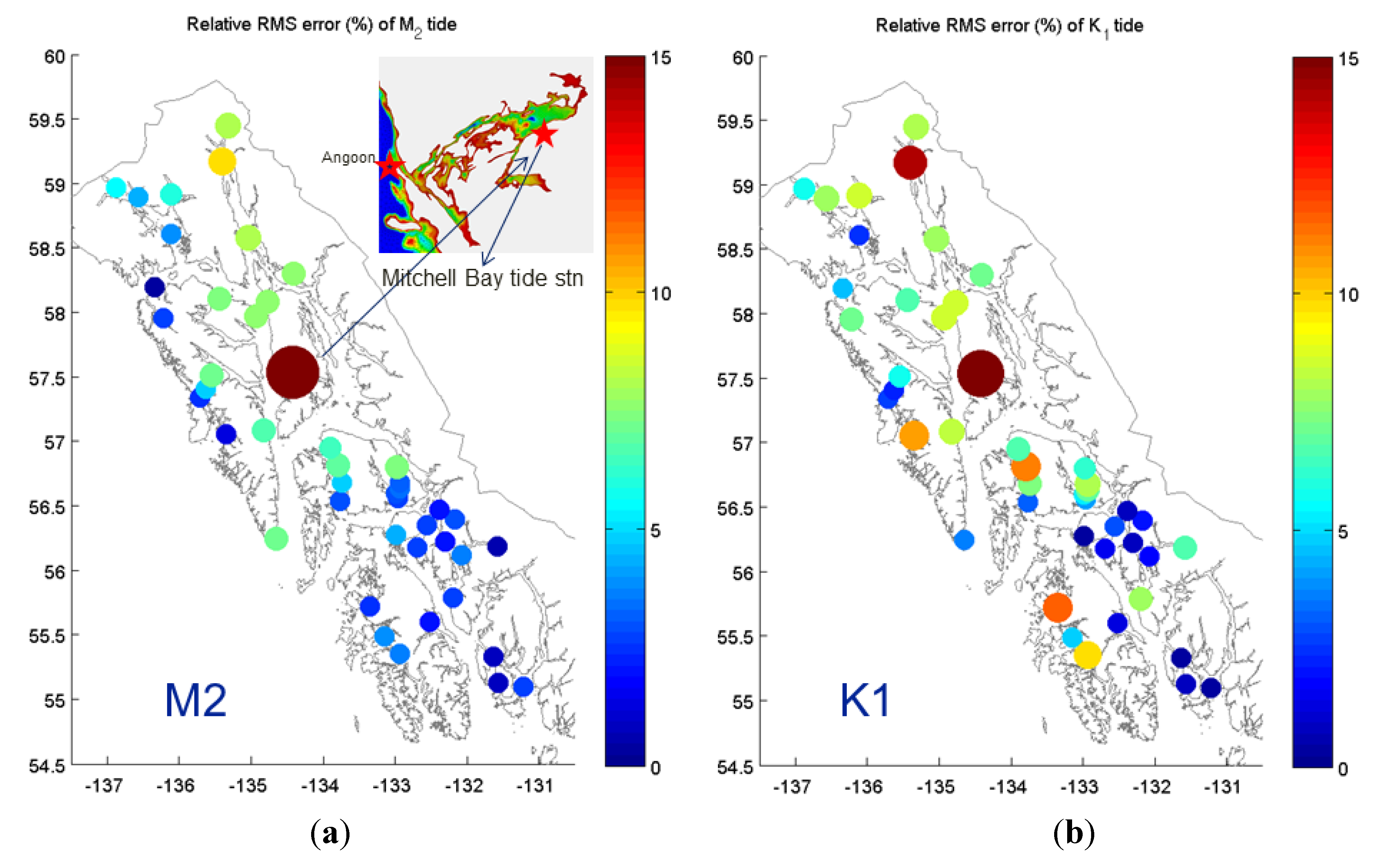
, will measure the relative model performance across the different tidal constituents. Mean RMSE and mean relative RMSE are the average RMSE and relative RMSE values over 43 tidal stations for one tidal constituent. The total mean RMSE (cm), Jmse 02 00171 i006, measures the RMSE of all tidal constituents.
The M2 tide has the smallest mean relative RMSE over all 43 data points (Table 1). K2 has the worst mean relative RMSE of all semidiurnal and diurnal tides, at 16.8%. All semidiurnal and diurnal tides have a mean relative RMSE between 5% and 10%, with the exception of the K2 tide. The M4 tide is inaccurate, with a mean relative RMSE of 54.4%. Most stations do not have MS4 and MN4 harmonic constant data, and thus, we do not present their performance statistics here. From the limited observed data points available for these constituents, MS4 and MN4 have similar relative RMSE as M4.
Table 1. Model-observation comparison: error measurements of nine tidal constituents, averaged over 43 tidal stations. MAE, mean absolute error; RMSE, root mean square error.
Amplitude error, MAE (cm)Phase error, MAE (degree)Mean RMSE (cm)Mean relative RMSE (%)
M28.292.939.475.5
S23.812.613.686.6
N21.633.532.146.3
K21.1411.802.5616.4
K12.964.713.907.9
O12.415.562.919.7
P10.626.031.358.3
Q10.313.820.386.6
M41.8226.111.6054.4
Total28.7
The model skill and performance have significant spatial variations across the 43 station points (Figure 5). Mitchell Bay, a 10 km2 in size inlet connected with Chatham Strait through a long, 100 m-wide narrow channel, is the location that the model performs the worst against the observations. The relative RMSE is well above 15% for all semidiurnal and diurnal tides here. At all other stations, the relative RMSE is usually below 10%.
Figure 5. Spatial distribution of relative RMSE (%). (a) M2; (b) K1.
Jmse 02 00171 g005

2.3. Discussion

For all the semidiurnal and diurnal tidal constituents, the SE Alaska model seems to overestimate the amplitude and underestimate the phase. For the M2 tide, the model results agree better with observations with low amplitudes and small phase lags (i.e., locations closer to the south open boundary) than the results with high amplitudes and large phase lags (i.e., locations inside passages and further away from the open boundary). Bottom friction can have a significant impact on the modeled tidal phase lags and amplitudes. There are many studies [4,23] evaluating the impact of bottom friction on phase lag and amplitude. Historically, the bottom friction used in VDatum tidal simulations has ranged from 0.001 to 0.00375 [13]. In our study, the bottom friction is set to a constant value, Cf = Cf (0.00375,0.00375). Besides the background run using this value, three more sensitivity tests were conducted with different values of bottom friction. Including the baseline run, the bottom friction coefficients for four test cases from low to high are Cf (0.00375,0.0020), Cf (0.00375,0.0025), Cf (0.00375,0.00375) and Cf (0.0045,0.0045). The total mean RMSE of nine tidal constituents (M2, S2, N2, K2, K1, O1, P1, Q1 and M4) in the four test cases were 29.7, 29.4, 28.7 and 28.7 cm, respectively. In general, the initial increase of bottom friction reduces the model amplitude and increases the phase lag of all tidal constituents, thereby slightly reducing the total mean RMSE. However, further increasing of the bottom friction to 0.0045 did not further reduce the error. The bottom friction coefficient, Cf (0.0045,0.0045), is larger than the values in previous VDatum tidal simulations and in other ADCIRC studies [21]. Furthermore, the model stability is too sensitive to further reduce the bottom friction coefficient. Therefore, no further sensitivity tests with lower or higher bottom friction coefficients were conducted. For semidiurnal tides, reducing the amplitudes and increasing the phase lags inside the passages is necessary to improve the model results. That implies a higher dissipation rate of tidal energy in the model inside the passages. Many studies [24,25] indicate the baroclinic tidal energy dissipation may play a more significant role than the bottom friction. A barotropic model may not be able to address the tidal dissipation associated with baroclinic processes.
For the diurnal tides, the model-data comparison (Figure 4) may suggest a shift in amplitude and phase. We compared the PO2009 database with the 1/16 degree resolution global tidal model, FES2012 [12], along the open boundary. The two databases are very consistent along the open boundary. The preliminary results using the same 11 tidal constituents from FES2012 as an open boundary condition indicate that FES2012 reduces the total mean RMSE by 1.5 cm, from 28.7 cm to 27.2 cm. There is marginal improvement, but the error distribution and pattern shown in Figure 4 is still the same.
Another source of error may come from inadequate bathymetric data processing. Two changes were made to the bathymetry to increase model stability. One was to reduce the maximum horizontal slope and the other was to smooth the bathymetry to reduce the formation of landlocked wet elements in the ADCIRC model. In the early stages of the model development, a vertical depth unit correction from feet to fathoms in about 5% of the sounding data reduced the total mean RMSE by half. Any changes made to the bathymetry to help model stability may compromise the accuracy of the model. In Mitchell Bay, the grid resolution is relatively low compared to the scale of the narrow channel connecting the bay to Chatham Strait. There are only two rows of elements representing this narrow channel. In combination with the low resolution of DEM data here, the model overestimates tidal energy propagated into the bay from Chatham Strait.
The biggest challenge of tidal modeling in SE Alaska has been with the model’s numerical stability. The model can be unstable in wetting/drying scenarios involving landlocked wet elements. Figure 6 shows a time sequence of tidal elevations and velocities about one hour before the simulation ends due to the instability. The wet cells can connect with the open water episodically with a period of a few minutes, even as the tides are receding. The connection of these wet cells with the open water can be very abrupt. As the wetting/drying connection/disconnection process repeats, the outflow velocity increases until, eventually, the simulation fails. If the process has neutral or negative feedback, it may remain stable. In order to achieve model stability, the current model bathymetry had been smoothed aggressively. The bottom friction coefficient for shallow water less than 100 m is set to 0.00375, which is relatively large compared with other VDatum tidal modeling cases [13]. To achieve numerical stability without over-tuning the model’s physical parameters and bathymetry is the direction in our continued efforts to improve the model results.
Overall, with a minimum of 50-m spatial resolution, the SE Alaska tide model mesh grid is able to resolve complex waterways and passages in SE Alaska to reach all 43 current and historical tidal stations in the CO-OPS tidal database. The tidal model produces reasonable tidal results. Of all 11 tide constituents modeled (M2, S2, N2, K2, K1, O1, P1, Q1, M4, MS4 and MN4), three semidiurnal tides (M2, S2 and N2) and four diurnal tides (K1, O1, P1 and Q1) have a relative error below 10%. The K2 tide has a higher relative RMSE of 16.4%, and the M4 tide has a relative RMSE of 54.4%. The MN4 and MS4 tides do not have enough observational data to calculate the mean RMSE, but we expect the relative error to be large. The model generally overestimates the amplitude and underestimates the phase. There are a few directions to improve the model results, for example, to give a more realistic bathymetry in the tidal zone and also to prescribe a better spatially varying bottom friction. The model has a few locations, especially in Mitchell Bay (Figure 5), where significant model-observation discrepancies exist. Usually, these are places where there is not enough grid resolution to resolve the coastal features and/or there is a lack of bathymetric data. In all of these cases, though, the model can produce a reasonable phase, but an inaccurate amplitude (it is not be able to calculate an accurate energy influx). In future work, the tidal energy flux and dissipation in SE Alaska will be more thoroughly investigated with the model.
Figure 6. Time sequence of the modeled elevation and velocity field around landlocked wet elements. The simulation started using a restart file 65 min before failure.
Jmse 02 00171 g006

3. Use of Existing Tide Model Outputs in Western Alaska to Support Hydrographic Surveys

3.1. Introduction

During the development of the SE Alaska tide model, an existing model (FM) developed by Foreman et al. [16] in western Alaska was selected to evaluate how model results could improve tidal interpolation for hydrographic survey planning. The model domain covers a region of the Bering Sea where NOAA has planned upcoming survey operations. For the application to nautical charts, real-time sounding depths need to be corrected to a fixed vertical datum, such as mean lower low water (MLLW), as real-time sounding depths are impacted by non-tidal and tidal water level fluctuations. The tide correctors for both non-tidal and tidal components are derived from interpolated/extrapolated tidal fields of coastal station observations. CO-OPS’ HPT team generates tide correctors from coastal stations using the Tidal Constituent And Residual Interpolation (TCARI) software. TCARI works by solving Laplace’s equation constrained by boundary conditions to spatially interpolate tidal constituents, datums and water level residuals (i.e., the non-tidal component or the difference between the astronomically predicted tide and the observed water level) over an unstructured triangular grid [26,27]. Once the TCARI solution is completed for a grid, the water level data series can be derived at any given point within the grid.
The current method of interpolating/extrapolating onshore tidal observations for hydrographic surveys works well for the nearshore areas with substantial coastal stations and relatively simple tidal changes, as tidal features there can be readily captured by available coastal observations. However, in the Bering Sea of western Alaska, tides are very complex, due to the presence of amphidromic points and significant tidal amplification or reduction in coastal bays, estuaries and rivers. It is a challenge to accurately capture tidal propagation features in this region by relying only on the interpolation and extrapolation of the sparse onshore observed data [28].

3.2. Methods and Results

In this study, we examined the method of combining coastal observations with the tide model results. We first evaluate the FM performance at CO-OPS tide stations by comparing the modeled harmonic constants with observations. We then selected a number of offshore model points to be combined with onshore stations for the interpolation of harmonic constants using TCARI.
Figure 7. The spatial distribution of the relative RMSE (%) of Foreman’s model (FM) for (a) M2; and (b) K1.
Jmse 02 00171 g007
To quantify the FM performance and skill, we calculated the RMSE of tidal constituents at 18 CO-OPS coastal stations using Equation (2) from Section 2.2. The M2 RMSE ranges from 0.7 cm to 35.4 cm with an average of 10.7 cm. The K1 RMSE ranges from 0.7 cm to 16.7 cm, with an average of 4.5 cm. The relative RMSE (Figure 7) ranges from 2.5% to 177.7% for the M2 constituent and ranges from 3.8% to 85.4% for K1. Generally, the modeled tidal harmonics are comparable to the onshore observations, but have significant differences for particular stations. The discrepancies may be due to the relatively coarse resolution in particular regions and/or the absence of the local mass conservation of the model [16]. Given these discrepancies, accurate hydrographic surveys cannot rely only on the model outputs, especially in some nearshore regions. In this study, we propose to select a limited number of offshore model points to be combined with the onshore stations for interpolation, so that the interpolated harmonic constants in the nearshore regions are mainly controlled by the onshore observations.
A triangular mesh with 69,369 nodes and 112,575 elements with the resolution varying from a few meters to 30 km was developed for TCARI interpolation. This mesh has much higher resolution around the coast than the offshore regions, which helps to better capture tidal variations in the nearshore regions. The harmonic constants at a total of 18 CO-OPS stations and 21 model points in the domain (Figure 8) were used for interpolation.
Figure 8. (a) Study domain; (b) Center for Operational Oceanographic Products and Services (CO-OPS) tidal stations (blue squares), selected FM points (purple dots) and the literature stations from Pearson et al. [29] and Mofjeld [30] (brown triangles) in the domain. The thick black lines indicate the outer boundary of the triangular mesh used for Tidal Constituent and Residual Interpolation (TCARI) interpolation.
Jmse 02 00171 g008
The co-amplitude and co-phase tidal fields of six constituents (M2, S2, N2, K1, O1 and P1) are populated from a combination of the observed and modeled data using TCARI. The amplitudes (A) and phases (h) at the CO-OPS stations and the model points were first transformed into two variables: Acosh and Asinh, since it is difficult to directly interpolate phases with a range of zero to 360 degrees around amphidromic points. The values of Acosh and Asinh were then populated onto the triangular mesh using TCARI. Finally, the interpolated Acosh and Asinh fields were transformed back to amplitudes and phases.
Figure 9. M2 co-amplitude (left side panels) and co-phase (right side panels) contours from TOF (a,b); TO (c,d); and FM (e,f).
Jmse 02 00171 g009
Figure 10. K1 co-amplitude (left side panels) and co-phase (right side panels) contours from TOF (a,b); TO (c,d); and FM (e,f).
Jmse 02 00171 g010
As examples, the M2 and K1 co-amplitude and co-phase contours from TCARI interpolation of combined onshore CO-OPS observations and offshore FM outputs (the combination is referred to as TOF) are shown in Figure 9a,b and Figure 10a,b, respectively. As comparisons, the co-tidal contours from TCARI interpolation of only onshore CO-OPS observations (referred as TO) are shown in Figure 9c,d and Figure 10c,d. With the FM author’s permission, the co-tidal contours from FM are shown in Figure 9e,f and Figure 10e,f. The co-tidal contours from TOF are generally consistent with those from FM, but are different in the nearshore regions. The co-tidal contours from TOF are quite different from the TO contours, especially in terms of the presence and the location of the amphidromes.
From the TO M2 contours (Figure 9c,d), there is no amphidromic point at the northern part of the Bristol Bay entrance. The co-amplitude and co-phase lines in Bristol Bay tend to be perpendicular to the longitudinal axis of the bay, suggesting rectilinear tidal propagation. From the TOF M2 contours (Figure 9a,b), an amphidromic point appears at the north part of the Bristol Bay entrance, which is consistent with the FM M2 contours (Figure 9e,f) and indicates the more realistic presence of rotational tidal propagation. The magnitude of the TOF M2 amplitudes in the bay is also more realistic than the TO M2 amplitudes. In addition, compared to the TO contours, the M2 tide features in Norton Sound become clearer and more realistic in the TOF contours. The offshore M2 patterns have been changed even more significantly in terms of both amplitude and phase, since more model points are involved in the interpolation relative to the nearshore regions.
For the K1 constituent, an amphidromic point to the south of Nunivak Island is only present in the TOF contours (Figure 10a,b). The K1 co-amplitude lines from TOF in Bristol Bay are thus more narrowly spaced than those from TO. In addition, a second K1 amphidromic point at the Norton Sound entrance shown in the TO contours (Figure 10c,d) is moved northward onto the land in the TOF contours. However, the K1 co-amplitude lines are not considerably altered from TO to TOF.

3.3. Discussion

Due to the scarce nearshore observations, it is difficult to directly evaluate the FM results and the interpolation results in the nearshore regions of interest to hydrographic surveys. However, there are some historic observed data available at offshore sites from Pearson et al. [29] and Mofjeld [30]. These two studies provide third-source data to be compared with the FM results and the interpolation results. The observed data and the offshore sites in these two studies will be referred to as the literature observations and the literature stations in the next discussion. The location and name of the literature stations are shown in Figure 8b. For each of the literature stations, we extract harmonic constants from the FM results and the interpolation results to be compared with the literature observations. The results for M2 and K1 are listed in Table 2 and Table 3, respectively. In these two tables, the station names are the same as listed in the original literature. OBS refers to observed data (stations LD14A, NC17C, NC19C, and LD10A, Table 2) from Mofjeld [30] and observed data (all other stations) from Pearson et al. [29]. The RMSEs relative to OBS have been calculated using Equation (2) in Section 2.2 for FM, TO and TOF individually at each literature station.
Table 2. Comparisons of M2 amplitude and phase at the literature stations between observed data (OBS), FM, TO and TOF. The acronyms have been described in the text.
StationLatitude
(°N)
Longitude
(°W)
Amplitude (cm)Phase (°)RMSE (cm)
OBSFMTOTOFOBSFMTOTOFFMTOTOF
BC2060.43171.0820.526.448.731.0171.0169.9144.8177.04.144.37.7
BC355.02165.1741.942.752.039.889.084.579.389.52.422.31.5
BC13B55.50165.8235.537.354.938.7106.099.186.2102.23.430.02.9
BC13D55.78165.3839.041.059.840.6109.0109.391.6108.81.433.71.1
BC1057.28169.5524.928.947.130.7131.0119.498.3117.14.732.96.2
BC458.62168.2333.435.757.735.1151.0145.0121.3151.83.046.41.2
FX258.53167.9333.835.758.835.0158.0145.0121.9151.05.747.33.1
BC959.22167.7036.738.159.836.1164.0157.3135.8169.93.353.02.7
BC1159.70167.2535.938.360.837.0155.0161.1146.2182.53.257.012.3
BC2160.38169.1830.936.851.835.6189.0186.2152.8185.24.351.63.7
BC755.70163.0271.473.275.156.5134.0133.0118.6125.91.541.512.3
BC257.07163.3745.243.682.556.1157.0157.9141.0147.31.269.39.7
BC1557.65162.7036.233.790.958.2168.0170.9156.5157.12.280.316.8
LD162.50166.1246.144.230.322.9328.0325.076.3327.02.217.716.4
NC1762.88167.0825.625.829.721.7330.0322.7200.2298.82.339.19.4
NC1863.15168.3822.420.230.421.1324.0314.9246.7272.32.834.713.5
LD263.22168.5826.622.030.221.5319.0313.4253.9271.03.636.814.2
LD464.78166.834.93.816.912.9138.0162.7191.8219.41.515.49.2
GEO
PROBE
64.00165.5013.011.418.414.444.032.535.415.62.15.74.8
LD564.13163.002.05.617.915.9233.0162.0230.3168.43.713.710.7
LD14A60.57170.6021.927.848.831.3180.0177.0149.0181.14.345.56.6
NC17C62.88167.0725.525.929.621.7336.0323.0198.4299.14.138.910.9
NC19C64.00172.3323.525.228.520.3172.0181.9201.7200.43.236.87.9
LD10A65.58168.637.69.816.011.3202.0211.7199.8208.31.816.62.7
Average 3.037.97.8
Overall, FM has the best performance, since this model has assimilated offshore altimetry data and most of the literature stations are located offshore. TO has the worst performance, suggesting that it is unreliable for capturing complex offshore tidal features by the interpolation of onshore observations only. On the other hand, TOF significantly improves the results relative to TO for almost all literature stations, confirming that TOF is a better option than TO for supporting hydrographic surveys. The only exceptions are the K1 comparisons (Table 3) at BC3, BC7, LD4 and LD5, where TOF is slightly worse than TO, indicating that the interpolated K1 values at these stations should be mainly controlled by the onshore observations.
The M2 comparisons at seven stations (BC3, BC13B, BC13D, BC4, FX2, BC9 and BC21) show that TOF has the best performance, indicating that interpolation from combined onshore observations and offshore model outputs is a promising method. However, the M2 comparisons at other stations (especially BC11, BC7, BC2, BC15, LD1, NC18, LD2, LD4 and LD5) show that TOF performs worse than FM. This may be due to the inadequate number or the inappropriate distribution of selected model points in the vicinity of these literature stations.
Table 3. Comparisons of K1 amplitude and phase at the literature stations between OBS, FM, TO and TOF. The acronyms have been described in the text.
StationLatitude
(°N)
Longitude
(°W)
Amplitude (cm)Phase (°)RMSE (cm)
OBSFMTOTOFOBSFMTOTOFFMTOTOF
BC2060.43171.0818.119.730.521.5326.0322.8337.6315.61.49.43.5
BC355.02165.1740.942.242.836.5319.0315.6322.3323.72.02.23.8
BC13B55.50165.8234.436.943.034.2325.0323.7329.3328.61.96.41.5
BC13D55.78165.3833.435.944.634.6327.0327.9334.0333.01.88.62.7
BC1057.28169.5524.926.936.725.8333.0327.8332.8322.32.28.43.4
BC458.62168.2312.412.438.120.8303.0301.1339.7310.40.320.66.1
FX258.53167.938.911.038.821.3288.0299.7340.9313.12.124.29.7
BC959.22167.709.710.837.922.7258.0255.1342.9290.80.927.110.9
BC1159.70167.2518.318.037.322.5207.0219.2343.1263.92.736.814.0
BC2160.38169.1816.618.231.420.5297.0296.6336.7298.51.115.22.8
BC755.70163.0249.051.850.844.0335.0331.7348.4352.22.98.310.4
BC257.07163.3728.327.952.443.113.013.73.919.00.317.610.8
BC1557.65162.7029.931.555.549.548.049.020.643.71.222.714.0
LD162.50166.1231.730.920.617.9324.0333.616.6356.53.817.813.6
NC1762.88167.0819.019.219.416.2341.0347.910.6353.11.66.93.3
NC1863.15168.388.911.717.313.6356.0358.6358.8349.52.06.03.4
LD263.22168.588.110.916.613.0359.04.5358.7350.52.16.03.6
LD464.78166.834.20.99.97.9222.07.4264.4320.13.55.26.7
GEO
PROBE
64.00165.5014.013.316.716.071.063.4118.474.61.48.91.6
LD564.13163.0032.126.628.830.2110.0119.2112.198.55.12.44.6
LD14A60.57170.6017.218.930.220.8322.0318.2337.8312.71.510.23.4
NC17C62.88167.0718.519.319.416.2346.0348.010.8353.30.75.82.2
NC19C64.00172.339.911.414.310.9328.0329.7326.9334.51.13.11.1
LD10A65.58168.632.73.36.64.5359.0322.6276.1304.31.44.82.6
Average 1.911.95.8
The experiments presented here are the initial step for integrating tide models and observations to better support hydrographic surveys. We are working on more sensitivity tests to determine the optimal number and locations of the model points that should be included in TCARI interpolation for further improvement. Further tests of the method may also help to determine where the new tide gauges should be installed to improve the regional interpolated tidal fields. The corresponding analysis and results will be reported in future work.
To further facilitate hydrographic survey planning, a series of tidal parameters, such as MN and HWI, are derived from the TOF amplitudes and phases of six tidal constituents using Form 180 [31]. Form 180 is an NOS CO-OPS’s standard procedure for estimating tidal parameters, including tidal datums, tidal ranges and tidal time intervals from tidal harmonic constants. In general, as shown in Figure 11, the patterns of MN and HWI are similar to the M2 amplitude and phase (Figure 9a,b), respectively, in semidiurnal tide dominated areas. MN has near zero values in the vicinity of the M2 amphidromic points and to the south of some islands. HWI, mainly representing the M2 phase, shows rotational tidal propagation at the Bristol Bay entrance and rectilinear tidal propagation within Norton Sound.
Figure 11. (a) The mean tidal range (MN) and (b) the high water interval (HWI) derived from TOF harmonic constants.
Jmse 02 00171 g011
The traditional co-tidal lines for hydrographic survey planning and the real-time water level time series for hydrographic surveys in an area of interest are developed mainly based on the interpolated fields of tidal harmonics and tidal parameters from coastal observations. This work could be potentially improved if the tidal constituents and tidal parameters are estimated in a more realistic way by adding offshore tide model results, especially in tidally complex areas. The methodology proposed in this study will be further tested for regions with more onshore observations and better understood co-tidal line patterns, such as in Chesapeake Bay and San Francisco Bay.

4. Summary and Future Work

NOAA’s VDatum program has a national tidal model development effort to systematically calculate spatially varying tidal datums. These high resolution tidal models [13] were developed using a finite element hydrodynamic model, ADCIRC, to simulate the tidal propagation in estuaries and coastal environments. The latest tidal modelling development effort in SE Alaska has approximately 2 million nodes with a minimum resolution of 50 m near the coast. The model is able to reach all 43 CO-OPS current and historical tidal stations in the modelling domain (Figure 1) for model validation. The SE Alaska tide model presented here has shown that tidal propagation characteristics are well represented with the ADCIRC model applied to the grid developed for this region. Of all 9 tide constituents (M2, S2, N2, K2, K1, O1, P1, Q1, and M4) used for model validation, three semidiurnal tides (M2, S2 and N2) and four diurnal tides (K1, O1, P1 and Q1) have a relative error below 10%. The K2 tide has a higher relative RMSE of 16.4%, and the M4 tide has a relative RMSE of 54.4%. The total mean RMSE (Table 1) for all 43 stations is 28.7 cm. A few model sensitivity tests have been conducted to test the model sensitivity to different bottom friction coefficients and to different prescribed boundary conditions. Further adjustments to this SE Alaska model will be focused on addressing the primary issues for model improvement, namely: (1) the general overestimation of amplitudes and the underestimation of phases; (2) local issues with accuracy due to local grid resolution and/or the lack of bathymetry; and (3) model stability in areas experiencing wetting/drying and associated development of landlocked wet cells in the grid. Overall, this model grid is quite advanced in that it has a significant amount of resolution to represent the numerous complex waterways throughout the Alexander Archipelago and associated coastal features. This grid and the model results will be invaluable in future VDatum representation of both regional and localized spatial variations in tidal datums.
While the primary output from the tidal models for VDatum has traditionally been used for computing tidal datums, new uses of modeled information should be more thoroughly evaluated. One such identified new use is to provide hydrographic survey planning with offshore tidal harmonic constants that can be integrated with tidal harmonic constants derived from observations in the TCARI interpolation. The western Alaska work presented here demonstrated a clear improvement of integrated offshore tidal harmonic constants over interpolated values based solely on tidal gauge data. The co-amplitude and co-phase contours of the M2 and K1 harmonic constituents are much more consistent with the contour output from FM by integrating modeled harmonic constants (Figure 9 and Figure 10). The RMSE between the interpolated values and offshore observed values were improved from 37.9 cm to 7.8 cm for the M2 constituent and from 11.9 cm to 5.7 cm for K1 constituent by integrating modeled harmonic constants (Table 2 and Table 3). Further work will continue on sensitivity tests to determine the best approaches for selecting model points to use in this process, including the total number of points and their proximal location to amphidromes. The methodology will also be further examined using different tidal models, as well as new interpolation techniques, such as that developed by Shi et al. [32]. These tests will continue for the western Alaska domain, as well as for the VDatum tide models previously developed for other regions. The SE Alaska tide model will be used similarly as input to the process of updating contours of tidal information for hydrographic survey planning purposes.

Acknowledgments

We would like to extend our gratitude to Mike Foreman for making his tide model results available to help in the effort of assessing the impact of model results on improving the hydrographic planning process in the Bering Sea. Many thanks are given as well to the CO-OPS Hydrographic Planning Team for their collaboration on this effort in western Alaska. The Cartographic and Geospatial Technology Programs branch (in particular, Cuong Hoang and Kurt Nelson) of NOAA’s Coast Survey Development Laboratory (CSDL) and NOAA’s National Geophysical Data Center provided the bathymetry and DEMs needed for the ADCIRC grid in southeast Alaska. Doug Graham of NOAA’s National Geodetic Survey assembled the shoreline used in the development of this grid. We also thank Barry Gallagher of CSDL for providing assistance with the use of the TCARI program for the interpolation of tidal variables in western Alaska. We also would like to thank the anonymous reviewers, whose comments helped improve this manuscript.

Conflicts of Interest

The authors declare no conflict of interest.

References

  1. Parker, B.B.; Hess, K.W.; Milbert, D.G.; Gill, S. A national vertical datum transformation tool. Sea Technol. 2003, 44, 10–15. [Google Scholar]
  2. Vertical datum transformation. Available online: http://vdatum.noaa.gov/docs/standardprocedures.html (accessed on 18 Febuary 2014).
  3. Luettich, R.A., Jr.; Westerink, J.J.; Scheffner, N.W. ADCIRC: An Advanced Three-Dimensional Circulation Model for Shelves Coasts and Estuaries, Report 1: Theory and Methodology of ADCIRC-2DDI and ADCIRC-3DL; Dredging Research Program Technical Report DRP-92-6; U.S. Army Engineers Waterways Experiment Station: Vicksburg, MS, USA, 1992; p. 137. [Google Scholar]
  4. Westerink, J.J.; Blain, C.A.; Luettich, R.A., Jr.; Scheffner, N.W. ADCIRC: An Advanced Three-Dimensional Circulation Model for Shelves Coasts and Estuaries, Report 2: Users Manual for ADCIRC-2DDI; Dredging Research Program Technical Report DRP-92-6; U.S. Army Engineers Waterways Experiment Station: Vicksburg, MS, USA, 1994; p. 156. [Google Scholar]
  5. Foreman, M.G.G.; Crawford, W.R.; Cherniawsky, J.Y.; Henry, R.F.; Tarbotton, M.R. A high-resolution assimilating tidal model for the northeast Pacific Ocean. J. Geophys. Res. 2000, 105, 28629–28651. [Google Scholar] [CrossRef]
  6. Myers, E.P.; Baptista, A.M. Inversion for tides in the Eastern North Pacific Ocean. Adv. Water Resour. 2001, 24, 505–519. [Google Scholar] [CrossRef]
  7. Spargo, E.A.; Westerink, J.J.; Luettich, R.A.; Mark, D.J. ENPAC 2003: A Tidal Constituent Database for the Eastern North Pacific Ocean; Department of the Army Technical Note TR-04-12; U.S. Army Corps of Engineers: Washington, DC, USA, 2004. [Google Scholar]
  8. Hill, D.F.; Ciavola, S.J.; Etherington, L.; Klaar, M.J. Estimation of freshwater runoff into Glacier Bay, Alaska and incorporation into a tidal circulation model. Estuar. Coast. Shelf Sci. 2009, 82, 95–107. [Google Scholar] [CrossRef]
  9. Inazu, D.; Sato, T.; Miura, S.; Ohta, Y.; Nakamura, K. Accurate ocean tide modeling in southeast Alaska and large tidal dissipation around Glacier Bay. J. Oceanogr. 2009, 65, 335–347. [Google Scholar] [CrossRef]
  10. Egbert, G.D.; Bennett, A.F.; Foreman, M.G.G. TOPEX/POSEIDON tides estimated using a global inverse model. J. Geophys. Res. 1994, 99, 24821–24852. [Google Scholar] [CrossRef]
  11. Egbert, G.D.; Erofeeva, S.Y. Efficient inverse modeling of barotropic ocean tides. J. Atmos. Oceanic Technol. 2002, 19, 183–204. [Google Scholar] [CrossRef]
  12. Carrère, L.; Lyard, F.; Cancet, M.; Guillot, A.; Roblou, L. FES2012: A New Global Tidal Model Taking Advantage of Nearly 20 Years of Altimetry. In Proceedings of the Meeting 20 Years of Altimetry, Venice, Italy, 24–29 September 2012.
  13. Myers, E.P.; Yang, Z.; Xu, J.; Hess, K.W.; Dhingra, E. Tide Modeling in Support of NOAA’s National VDatum Program. In Estuarine and Coastal Modeling, Proceedings of 11th International Conference on Estuarine and Coastal Modeling, Seattle, WA, USA, 4–6 November 2009; Spaulding, M.L., Ed.; American Society of Civil Engineers: Reston, VA, USA, 2010; pp. 514–526. [Google Scholar]
  14. Liu, S.K.; Leendertse, J.J. Three-dimensional model of bering and chukchi sea. Coast. Eng. 1982, 18, 598–616. [Google Scholar]
  15. Kowalik, Z. Bering Sea Tides. In Dynamics of the Bering Sea; Loughlin, T.R., Ohtani, K., Eds.; University of Alaska Sea Grant: Fairbanks, AK, USA, 1999; pp. 93–127. [Google Scholar]
  16. Foreman, M.G.G.; Cummins, P.F.; Cherniawsky, J.Y.; Stabeno, P. Tidal energy in the Bering Sea. J. Mar. Res. 2006, 64, 797–818. [Google Scholar]
  17. OSU tidal data inversion. Available online: http://volkov.oce.orst.edu/tides (accessed on 18 Febuary 2014).
  18. NOAA NGDC. Integrated Models of Coastal Relief. Available online: http://www.ngdc.noaa.gov/mgg/coastal/coastal.html (accessed on 18 Febuary 2014).
  19. Amante, C.; Eakins, B.W. ETOPO1 1 Arc-Minute Global Relief Model: Procedures, Data Sources and Analysis; National Geophysical Data Center Marine Geology and Geophysics Division: Boulder, CO, USA, 2009; p. 19. [Google Scholar]
  20. Caldwell, R.J.; Eakins, B.W.; Taylor, L.A.; Carigna, K.S.; Collins, S. Digital Elevation Models of Southeast Alaska: Procedures, Data Sources and Analysis; National Geophysical Data Center Marine Geology and Geophysics Division: Boulder, CO, USA, 2010; p. 67. [Google Scholar]
  21. ADCIRC Related Publications. Available online: http://adcirc.org/home/documentation/adcirc-related-publications (accessed on 18 Febuary 2014).
  22. NOAA/NOS/CO-OPS—ODIN MAP. Available online: http://tidesandcurrents.noaa.gov/gmap3/index.shtml?type=TidePredictions&region= (accessed on 18 Febuary 2014).
  23. Lefèvre, F.; le Provost, C.; Lyard, F.H. How can we improve a global ocean tide model at a regional scale? A test on the Yellow Sea and the East China Sea. J. Geophys. Res. 2000, 105, 8707–8726. [Google Scholar] [CrossRef]
  24. Foreman, M.G.G.; Henry, R.F.; Walters, R.A.; Ballantyne, V.A. A finite element model for tides and resonance along the north coast of British Columbia. J. Geophys. Res. 1993, 98, 2509–2531. [Google Scholar] [CrossRef]
  25. Egbert, G.D.; Ray, R.D. Semi-diurnal and diurnal tidal dissipation from Topex/Poseidon altimetry. Geophys. Res. Lett. 2003, 30, 1907. [Google Scholar] [CrossRef]
  26. Hess, K.W. Spatial interpolation of tidal data in irregularly-shaped coastal regions by numerical solution of Laplace’s equation. Estuar. Coast. Shelf Sci. 2002, 54, 175–192. [Google Scholar] [CrossRef]
  27. Hess, K.W. Water level simulation in bays by spatial interpolation of tidal constituents, residual water levels, and datums. Cont. Shelf Res. 2003, 23, 395–414. [Google Scholar] [CrossRef]
  28. Lindley, C.; Urizar, C.; Wolcott, D.; Yang, H.; Huang, L. Vertical Control and Tide Reducers in Tidal to Non-Tidal Transitional Areas. In Proceedings of the U.S. Hydro2013 Conference, The Hydrographic Society of America, New Orleans, LA, USA, 25–28 March 2013.
  29. Pearson, C.A.; Mofjeld, H.O.; Tripp, R.B. Tides of the Eastern Bering Sea Shelf. In The Eastern Bering Sea Shelf: Oceanography and Resources; Hood, D.W., Calder, J.A., Eds.; University of Washington Press: Seattle, WA, USA, 1981; pp. 111–130. [Google Scholar]
  30. Mofjeld, H.O. Observed Tides on the Northeastern Bering Sea Shelf. J. Geophys. Res. 1986, 91, 2593–2606. [Google Scholar] [CrossRef]
  31. C&GS. Manual of Harmonic Constant Reductions; U.S. Government Printing Office: Washington, DC, USA, 1952; p. 74. [Google Scholar]
  32. Shi, L.; Hess, K.W.; Myers, E.P. Spatial interpolation of tidal data using a multiple-order harmonic equation for unstructured grids. Int. J. Geosci. 2013, 10, 1425–1437. [Google Scholar]

