The Storm Surge and Sub-Grid Inundation Modeling in New York City during Hurricane Sandy

Abstract

Hurricane Sandy inflicted heavy damage in New York City and the New Jersey coast as the second costliest storm in history. A large-scale, unstructured grid storm tide model, Semi-implicit Eulerian Lagrangian Finite Element (SELFE), was used to hindcast water level variation during Hurricane Sandy in the mid-Atlantic portion of the U.S. East Coast. The model was forced by eight tidal constituents at the model’s open boundary, 1500 km away from the coast, and the wind and pressure fields from atmospheric model Regional Atmospheric Modeling System (RAMS) provided by Weatherflow Inc. The comparisons of the modeled storm tide with the NOAA gauge stations from Montauk, NY, Long Island Sound, encompassing New York Harbor, Atlantic City, NJ, to Duck, NC, were in good agreement, with an overall root mean square error and relative error in the order of 15–20 cm and 5%–7%, respectively. Furthermore, using large-scale model outputs as the boundary conditions, a separate sub-grid model that incorporates LIDAR data for the major portion of the New York City was also set up to investigate the detailed inundation process. The model results compared favorably with USGS’ Hurricane Sandy Mapper database in terms of its timing, local inundation area, and the depth of the flooding water. The street-level inundation with water bypassing the city building was created and the maximum extent of horizontal inundation was calculated, which was within 30 m of the data-derived estimate by USGS.

1. Introduction

On 29 October 2012, around 7:30 pm EDT (UTC-4), Hurricane Sandy made landfall near Brigantine, NJ, and resulted in an enormous impact on life and property damage, with the estimated cost exceeding $50 billion along the eastern seaboard. The storm surge created some of the most devastating impacts, including flooding in New York City’s subway tunnels, LaGuardia and Kennedy airports, damage to the New Jersey transit system, and the coastal seashore [1].

Hurricane Sandy was formed in the Caribbean Sea on 22 October 2012. It strengthened as it moved northwards and was a Category 2 hurricane at its peak. On October 28, as it passed through the mid-Atlantic Bight, the hurricane began to make a hard turn to the northwest because of the large-scale wind flow pattern favoring an upper-level blocking over Greenland and a mid-level trough coming from the U.S. southeast. As a result, Hurricane Sandy made a landfall as a Category 1 hurricane on the New Jersey coast, impacting highly populated urban areas including nearby New York City. When it made landfall, an abnormal storm tide with catastrophic, record-setting water levels occurred in New Jersey, New York City and in a portion of Long Island Sound. The NOS tide gages records show water level at The Battery, NY, Bergen Point, NY, Sandy Hook, NJ, Bridgeport, CT, New Haven, CT, at 2.74, 2.90, 2.44, 1.77, and 1.69 meters above mean higher high water, respectively [1]. The worst flooding occurred over Staten Island and to the south along the New Jersey shore. The storm surge also caused significant flooding in parts of the Hudson River Valley, the East River, and the western part of Long Island Sound.

Many storm surge models have been developed and applied in the U.S. coastal regions; they vary either by structured/unstructured grids or by different numerical schemes used. Examples are: Sea, Lake, and Overland Surges form Hurricanes (SLOSH) [2], ADCIRC [3], FVCOM [4], CH3D-IMS [5], and CEST [6]. SELFE is a semi-implicit finite element model developed by [7] using the Eulerian-Lagrangian scheme, which is not restricted by the CFL (Courant-Friedrichs-Lewy) condition, and thus allows large time steps and robust computations. The 2-D mode of Semi-implicit Eulerian Lagrangian Finite Element (SELFE) was applied for the Hurricane Sandy simulation in a large-scale domain covering the entire U.S. East Coast. The purpose of the large domain model is to ensure that the storm tide driven by Hurricane Sandy from the ocean is accurately simulated in the major estuaries and waterways at the coast, where the model results can be evaluated by NOAA tidal gauge data. At the same time, it also provides boundary conditions for a separate, high-resolution, sub-grid inundation model designed specifically for the New York City metropolitan area. This is needed because the risk of inundated area per capita population is very high in the urbanized city. As a result, a highly resolved, accurate sub-grid inundation model UnTRIM² [8], which incorporates LIDAR (Laser Imaging Detection and Ranging) data directly into the sub-grid, was set up to simulate the inundation of the city during Hurricane Sandy. With the resolution and accuracy, the street-level inundation was revealed and overall accuracy for the horizontal extent of the inundation was within 30 m mean absolute deviation (MAD) compared with the USGS Hurricane Sandy database. The remainder of the paper is organized as follows: in Section 2, the SELFE model setup is illustrated; the results of storm tide prediction are presented in Section 2.3. Section 3 describes the sub-grid inundation modeling paradigm and its setup in the New York City. The sub-grid model results are presented in Section 3.3. Finally, Section 4 discusses the results and concludes the paper.

2. Storm Tide Modeling along the U.S. East Coast

The SELFE (Semi-implicit Eulerian Lagrangian Finite Element) model developed by Zhang and Baptista in 2008 is a fully 3-D, baroclinic unstructured grid, coastal ocean model [7]. The 2-D barotropic mode, which assumes vertically-averaged horizontal velocities, was applied for the entire U.S. East Coast for the storm tide prediction during Hurricane Sandy. The model makes computations using global coordinates and has been parallelized using MPI (Message Passing Interface), thus making it suitable for large-scale calculations. Recent upgrades to the model include the improvements in the wetting and drying scheme, and coupling with the Wind Wave Model—WWM [9].

The model domain features a curvilinear open boundary stretching from Key West, Florida, to Nova Scotia in Canada at around 62°W (Figure 1). The finite element grid is comprised of 207,996 nodes and 392,013 elements, and extends from the U.S. East Coast out about 1500 km into the Atlantic Ocean. The spatial resolutions are from about 50 km at the grid’s open boundary near Bermuda to about 50 m in the Hudson River near NY Harbor. The model grid includes 134 open-boundary nodes, where the tidal constituent forcing can be applied from the open ocean far from the influence of a hurricane. Additionally, there are seven boundary nodes for applying river discharges from major rivers in the region with prescribed flux boundary conditions.

Figure 1. The Semi-implicit Eulerian Lagrangian Finite Element (SELFE) storm tide model domain covering the US East Coast from Key West to Nova Scotia at 62°W (left panel). The inset of the mid-Atlantic Bight portion of the US East coast with the NOAA tidal gauge stations used for model and data comparisons (right panel). Global tidal constituents were specified at the open boundary.

Figure 1. The Semi-implicit Eulerian Lagrangian Finite Element (SELFE) storm tide model domain covering the US East Coast from Key West to Nova Scotia at 62°W (left panel). The inset of the mid-Atlantic Bight portion of the US East coast with the NOAA tidal gauge stations used for model and data comparisons (right panel). Global tidal constituents were specified at the open boundary.

2.1. Wind Forcing Using RAMS Model

The high-resolution winds for Hurricane Sandy were produced from RAMS (Regional Atmospheric Modeling System) by WeatherFlow (http://www.weatherflow.com/). The wind field covers from Latitude 33.000 to 42.972 and Longitude from 78.000 to 68.026 with square elements of 2.16 arc-seconds (which is 4 km north-south by 3.4 km to 2.9 km east-west) with a 1-h temporal resolution. The duration of the wind and pressure field data provided is from October 24 00:00:00 GMT through October 31 00:00:00 GMT, 2012. This wind product is a continuous hindcast run in contrast to the normal 30 h forecast runs produced every 6 h. The product assimilates observations from many sources, including Weatherflow’s extensive network of meteorological stations. The SELFE model’s atmospheric forcing field requires a fully-expanded longitude-latitude grid, specific variable names, time units measured in days, and a time origin in a specific format. The atmospheric data provided by Weatherflow is in an interoperable NetCDF format, which can be adapted to the SELFE model with minimal preprocessing. A short script using NetCDF operators can augment and adjust the metadata of this Weatherflow product in less than 10 s to support the SELFE model setup. The wind drag coefficient used is the Garratt formulation [10]:

C_dw = (0.75 + 0.067W) × 10^-3

(1)

where W is the wind speed in m/sec. The C_dw is capped at the maximum value of 0.003 in Equation (1).

2.2. Open Boundary Conditions and Tidal Calibration

Eight global ocean tidal constituents, four semidiurnal constituents (M2, N2, S2, and K2) and four diurnal constituents (O1, P1, K1, and Q1), obtained via SMS (Surface-water Modeling System) version 8.0 by the FES95.2 global model formulation for harmonic tides [11] were used along the 134 nodes open boundary to force the tides along the eastern boundary. Factors that can reduce the tidal potential forcing due to the Earth’s tide were also accounted for in SELFE by the nodal factor and equilibrium arguments. The friction parameters were obtained based on the calibration with tidal elevations at 14 NOS stations: Montauk, NY; Newport, RI; New London, CT; New Haven, CT; Bridgeport, CT; Kings Point, NY; The Battery, NY; Bergen Point, NY; Sandy Hook, NJ; Atlantic City, NJ; Lewes, DE CBBT, VA; Sewell Point, VA; and Duck, NC. The results showed that the Manning’s n = 0.020 could be used for the majority of the areas in the domain except: (1) n = 0.01 for the Hudson River, New York Harbor, and Raritan Bay; and (2) n = 0.045 for the East River and its junction with the Hudson River. These latter values were consistent with a study in the New York Bight using the ECOM-3D model [12]. During the storm tide simulation, because tangential stress on the sea surface is large, the Reid (1957)’s modified bottom friction formula [13] was used to account for the effect of wind:

(2)

where C_db is the bottom drag coefficient, U is the vertically average velocity, τ_w the wind stress. The + is used when the U is opposing the wind and − is used when U is following the wind.

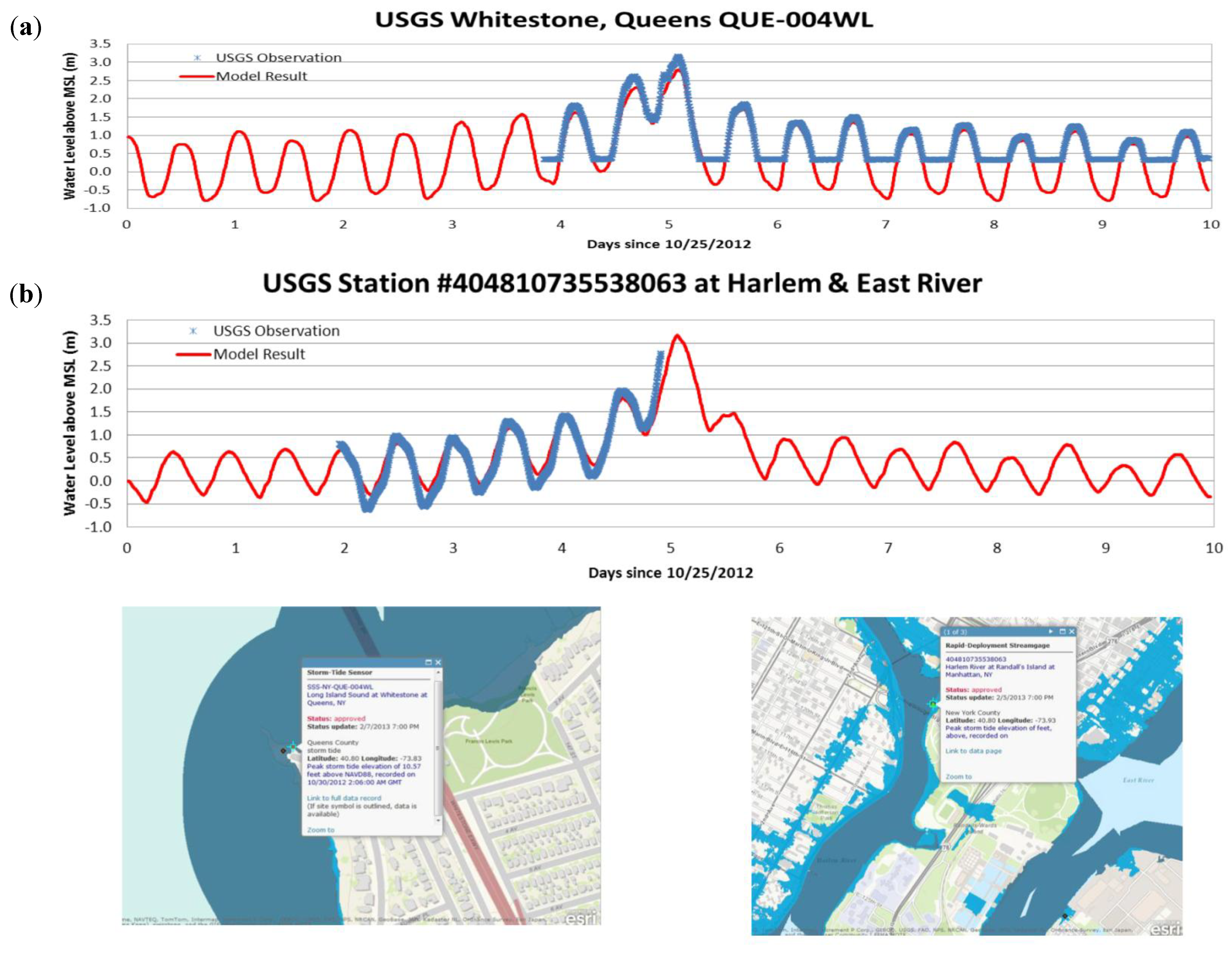
2.3. Storm Tide Hindcast for the U.S. East Coast

Hurricane Sandy made landfall near Atlantic City, NJ, USA, on 29 October 2012, around 23:30 GMT. The approaching hurricane generated wind fields, which had both local and remote effects. Given that the hurricane took the path along the offshore of the U.S. East Coast from the south to the north, the Eastern Seaboard experienced the remote wind effect before the hurricane made the landfall. In order to capture the buildup, the SELFE run started the spin up run with the tide only on October 12: 00:00:00 GMT for 3 days. The storm tide simulation then started (with the hot-start file) on October 15, 00:00:00 GMT for 16 days and ended on October 31, 00 00:00 GMT, 2012. For the early part of the storm tide period from October 15 to October 23, the model used NARR (North American Regional Reanalysis) wind and pressure fields every 3 h from the NOAA Earth System Research Laboratory. It was followed by the RAMS wind and pressure fields starting October 24, 00:00:00 GMT until it ended on October 31, 00:00:00 GMT. Figure 2a–c show the storm tide results at nine stations from Long Island Sound, NY, encompassing New York Harbor, to Duck, NC, during the period from October 28, 00:00:00 GMT to October 31, 00:00:00 GMT. Figure 2a is grouped with the stations in the Long Island Sound. Comparing the timing of the highest water level suggested that the surge started at Montauk, NY and propagated westward toward Kings Point, NY at which the storm tide reached the peak at around 3.2 m above mean sea level. The model performance was satisfactory with the correlation coefficient square (R²) above 0.94 and root mean square error (RMS) equal to 18 cm on average. It was noticed that there were phase discrepancies observed in the model at King’s Point, suggesting that some local effects contributed to the phase shift during the peak. Figure 2b was grouped with the station in the New York Harbor, at the entrance of the Harbor and in Atlantic City, NJ. Comparing the timing of the highest water levels suggested that there was a primary surge originating near Atlantic City and propagating north toward the Battery. The maximum storm tide height at the Battery reached 3.5 m above mean sea level, which is higher than that near where the storm made landfall, suggesting occurrence of amplification in New York Harbor. The model performance was again quite satisfactory with the correlation coefficient square (R²) above 0.95 and the root mean square error (RMS) around 17 cm on average. It is obvious that during Hurricane Sandy there were two storm surges converging upon New York City; one from Long Island Sound westward and the other from the New Jersey coast. Figure 2c groups the stations in Delaware, Virginia, and North Carolina, which are in the third and fourth quadrants of the hurricane track. While the northern stations were experiencing the maximum surge setup, these stations were actually experiencing set-down, as evidenced by the data, because of the offshore wind field. The model faithfully captured the dynamics correctly. The model performance in the region has a coefficient of determination (R²) above 0.90 and a root mean square error (RMS) around 18 cm on average. For Figure 2a–c, the mean absolute errors (MAE) are all below 15 cm except those at the stations: Lewes, DE, and Kings Point, NY. For Lewes DE, there were observation errors found in the measurement at Lewes, DE around October 30, 00:00:00 GMT, 2012 (in the time scale near day 3), and for Kings Point, an unexplained phase shift occurred near the maximum surge.

Figure 2. (a) Storm tide model results and data comparison for stations in Long Island Sound. Time series (left) and the statistical measures (right); (b) Storm tide model results and data comparison for stations near New York Harbor and Atlantic City, NJ, USA. Time series (left) and the statistical measures (right); (c) Storm tide model results and data comparison for stations in Delaware, Virginia and North Carolina, USA. Time series (left) and the statistical measures (right). The measurement errors are visible on day 3 at Lewes, DE, USA.

Figure 2. (a) Storm tide model results and data comparison for stations in Long Island Sound. Time series (left) and the statistical measures (right); (b) Storm tide model results and data comparison for stations near New York Harbor and Atlantic City, NJ, USA. Time series (left) and the statistical measures (right); (c) Storm tide model results and data comparison for stations in Delaware, Virginia and North Carolina, USA. Time series (left) and the statistical measures (right). The measurement errors are visible on day 3 at Lewes, DE, USA.

3. Sub-Grid Inundation Modeling in New York City

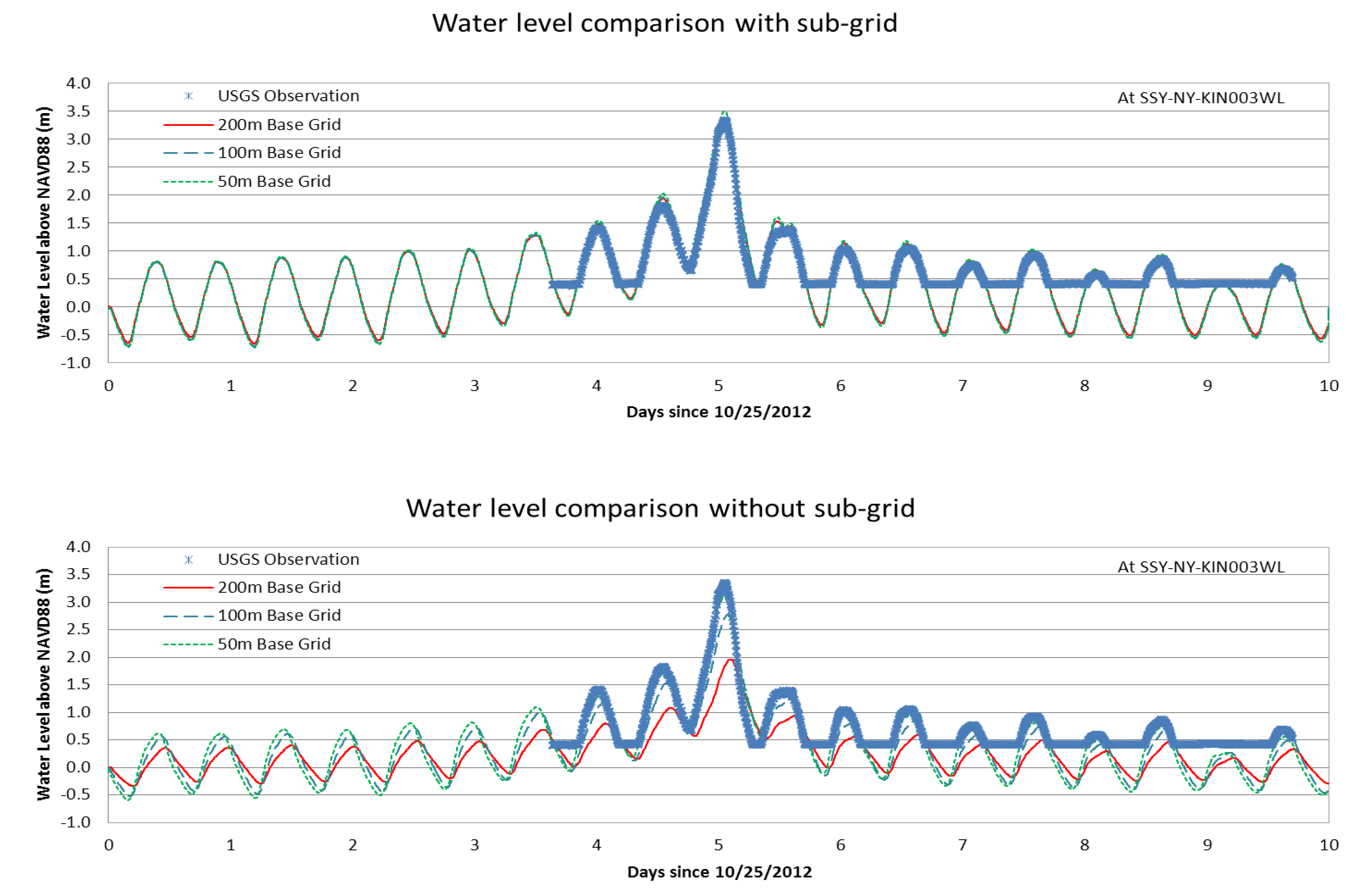
3.1. A New Paradigm for Inundation Modeling

When a hurricane surge floods into a city, it encounters land surfaces characterized by a wide range of features, from waterfront berms, streets, railroads, parks, highways to bridges, and building of different kinds. High-resolution hydrodynamic models are needed to simulate these local features. Even with the superior computing power available today, it is still insufficient to model these complex topographic features at the street and building scales. Given that LIDAR land data and water depths can now be collected with a very high resolution, it was recognized that the availability of detailed sub-element bathymetric data within a coarse computation grid should and can be used for further improving the model accuracy without having to use a fine computational mesh [14]. In this paper, a semi-implicit, semi-Lagrangian model: UnTRIM² was setup with the incorporation of LIDAR data in the sub-grid to simulate the inundation for New York City during Hurricane Sandy. It contains semi-implicit formulation and nonlinear solver for accurate simulating wetting and drying condition. The sub-grid friction and conveyance formulation were also included for the friction-dominated flow. The interested reader should refer to [8] and [14] for more detailed descriptions of the model feature. The basic concept of the sub-grid approach is to incorporate topographical details in a computational grid without having to make computations on the fine, sub-grid grid and hence achieve a fast computational runtime. For example, the sub-grid topography makes the co-existence of partially wet and dry regions, and the boundary, which separates the two, within a coarse computation grid possible. The end result is that the area calculation of a partially wetting and drying region can be determined more accurately instead of being designated as either completely wet or completely dry for the entire grid. In the same way, the cross-sectional areas perpendicular to the flow can also be obtained with higher accuracy by integrating slices of the sub-grid scale bathymetry across the flow face rather than based on one averaged depth for the entire flow face of a finite volume grid. In this way, more accurate flux calculation for the conveyance of the flow is achieved. In a friction-dominated flow, sub-grid bathymetry resolution can be further incorporated into the flow resistance formula to account for detailed bottom location and local bottom shear stress [8,15]. The formulation is briefly explained as follows. Let us assume that a 2-D flow is frictional dominated and thus the pressure gradient term is balanced by the friction term in the momentum equation at each time step:

(3)

where g is gravity, ζ is water surface elevation, cf is the friction parameter for which formulation can be given such as Chezy, where U is the velocity vector, and ||U|| is the magnitude of the velocity in Equation (3). This leads to:

(4)

where Ω is defined as conveyance velocity in Equation (4). If we assume that the pressure gradient is constant in the coarse grid cell during one time step, then given the fixed h and cf, it will lead to a single constant averaged velocity. On the sub-grid cell level, however, the velocity fields can vary because of the differences in the sub-grid bathymetry and the conveyances. If we assume that every sub-grid has the same surface size, then each sub-grid velocity will obey:

(5)

where j is the index for each sub-grid cell; h_j and u_j are the sub-grid depth and velocity, respectively. The sub-grid velocities u_j can be determined by ||U||, Ω of the coarse grid, and cf_j, and h_j, as follows:

(6)

where:

(7)

Therefore, the sub-grid level velocities and bottom stress can be obtained from the associated quantities at the coarse grid level through a simple algebraic relationship. These sub-grid information are integrated subsequently into the semi-implicit algorithm for the computation grid, permitting a substantial improvement of model accuracy without an overly expensive computational cost.

3.2. Sub-Grid Model Setup for New York City

In this study, the sub-grid hydrodynamic modeling effort was applied to research high-resolution street-level spatial inundation modeling in the New York Harbor region during Hurricane Sandy (2012). The sub-grid model domain encompasses the Hudson River up to Yonkers, the Harlem River, parts of Long Island Sound up to King’s Point, the East River and each of its tributaries (Figure 3a). Given that the New York City (NYC) building infrastructure is generally arranged in a block system, the grid developed using LIDAR-derived data has been scaled to square grids relatively congruent to the native resolution of the topographic data contained in the DEM (Digital Elevation Model, which is retrieved from the USGS National elevation dataset). The model grid designed for the New York City simulation makes use of a 200 m × 200 m square base grid and in each of the base grid, there are 40 by 40 numbers of 5 m × 5 m sub-grids embedded within each base grid cell (Figure 3b). To retain the accuracy, the uniform square grid LIDAR-derived data were imported directly into the sub-grid. When coupled with a nonlinear wetting and drying solver [14], the shoreline is intrinsically resolved in the sub-grid which allows partial wetting and drying within a coarse grid when the water level changes at with time step. The Open NYC Building Inventory is extremely important in the city landscape and was added separately to the DEM, and is resolved by the sub-grids (see right panel, Figure 3). The bathymetric and topographic data sources used in New York City are shown in Table 1.

Figure 3. (a) The sub-grid inundation modeling domain in New York City covering the Hudson River up to Yonkers, the Harlem River, part of the Long Island Sound up to King’s Point and each of their tributaries, shown in base grids. (b) The sub-grid 5 m by 5 m embedded in the 200 m × 200 m resolution base grid over the shaded area in lower Manhattan (right) including “The Battery”. The LIDAR data are directly imported into the uniform square sub-grids to resolve the building and the street.

Figure 3. (a) The sub-grid inundation modeling domain in New York City covering the Hudson River up to Yonkers, the Harlem River, part of the Long Island Sound up to King’s Point and each of their tributaries, shown in base grids. (b) The sub-grid 5 m by 5 m embedded in the 200 m × 200 m resolution base grid over the shaded area in lower Manhattan (right) including “The Battery”. The LIDAR data are directly imported into the uniform square sub-grids to resolve the building and the street.

Table 1. Data sources of the bathymetry and LIDAR topography used as inputs in the sub-grid.

	Bathymetry Data	Resolution	Area
Bathymetry	NOAA Coastal Relief Model	3 arc s (≈90 m)	Coastal Regions
	NOAA Bathymetric Survey Data	1/3 arc s (≈10 m)	Hudson River, East River, Kill van Kull, Raritan Bay, and New York Bay
Topography	USGS National Elevation Dataset	1/3 arc s (≈10 m)	Low-elevation areas around the New York Harbor and Raritan Bay
	USGS National Elevation Dataset	1/9 arc s (≈3 m)	Select areas of New York City
	Open NYC Building Inventory	0.1 m	New York City Buildings

Table 1. Data sources of the bathymetry and LIDAR topography used as inputs in the sub-grid.

	Bathymetry Data	Resolution	Area
Bathymetry	NOAA Coastal Relief Model	3 arc s (≈90 m)	Coastal Regions
	NOAA Bathymetric Survey Data	1/3 arc s (≈10 m)	Hudson River, East River, Kill van Kull, Raritan Bay, and New York Bay
Topography	USGS National Elevation Dataset	1/3 arc s (≈10 m)	Low-elevation areas around the New York Harbor and Raritan Bay
	USGS National Elevation Dataset	1/9 arc s (≈3 m)	Select areas of New York City
	Open NYC Building Inventory	0.1 m	New York City Buildings

Tides are forced via three open boundaries, one to the south, one to the west, and one to the east. The southern open boundary in the sub-grid domain is located at the mouth of the New York Bay into the Raritan Bay leading to the Atlantic Ocean. The open boundary to the west is Bergen Point (NOAA Station #8519483) where the Kill van Kull connects Newark Bay to New York Bay. The third open boundary is near Kings Point (NOAA Station #8516945) which lies to the east and connects the East River to Long Island Sound. Hourly fresh water flows for the Hudson River were obtained from USGS and specified as a flux distributed along nine elements at the northern boundary of the model domain near Wappingers Falls (Station #01372500). Atmospheric data were collected from NOAA atmospheric observation data at Bergen Point (Station #8519483). Atmospheric pressure was prescribed uniformly throughout the domain similar to that prescribed for wind. A Manning’s n value of 0.025 was determined to be used throughout the Hudson River and New York Bay except in the East and Harlem Rivers after the sub-grid model was calibrated with the astronomical tide data. A slightly higher Manning’s n value of 0.035 for the East and Harlem River was needed because the river was narrow, winding and contained many man-made features. After the forcing and the friction parameters were determined, the sub-grid model simulation was executed on a Dell Precision T-3500 with Intel Xeon W3670, Windows 7, 64-bit OS and 24 GB RAM. The CPU (Central Processing Unit) to real time ratio was roughly 240:1. Excellent storm tide results were obtained with a correlation coefficient of 0.98 compared with observed data from The Battery, NY NOAA tidal gauge station. Additional comparisons with the USGS rapid deployment gauges will be presented in the next section.

3.3. Sub-Grid Inundation Model Results Compared with USGS Hurricane Sandy Mapper

Aside from the modeling effort described so far, the USGS has made large efforts in deploying a monitoring network of water-level and pressure sensors along the U.S. Atlantic Coast during Hurricane Sandy [16]. These data combined with the field-verified high water marks collected post-storm were utilized to construct a water surface elevation, which was subsequently subtracted from the best available DEM to create a contour of the maximum extent of inundation, comprised of the inundation grid and surge boundary. The database and GIS (Geographic Information System) products produced by the USGS are tremendously valuable for benchmarking of the sub-grid model results.

3.3.1. Time Series Comparison—Timing of the Inundation

One of the means for verifying model performance is the use of time series comparisons at fixed spatial points. Figure 4a and Figure 5a,b show the comparison of sub-grid modeled storm tide results at three separate locations: Gowanus Canal, Brooklyn, Whitestone, Queens, and Lower Harlem, at the East River, where rapid deployment gauges were installed. In all three comparisons, it can be seen that the model-simulated results (shown in red) are consistent with the measured data (shown in blue) both in terms of the timing and the amplitude. The root mean square statistics for the above stations are 7.7 cm, 9.2 cm and 16.8 cm, respectively (note, only partial records are available at the station in lower Harlem at East River). In Figure 4a and Figure 5a, the gauge was set at a fixed height above the ground, which can become dry when the water falls below the gauge. What makes this comparison unique is that these stations are not permanently wet. That means the numerical wetting and drying scheme was quite robust and faithful in tracking the timing of the wetting and drying status revealed by the gauge. From the record, it is obvious that the inundation co-oscillated with the tidal cycle and that the model captured the timing and the depth of the water quite satisfactorily.

3.3.2. Thickness of the Inundation

When simulating inundation for the urban area such as the metropolitan area of New York City, one of the key parameters that needs to be determined is the flow resistance that includes the effects of high rise buildings and the streets. Since the flow resistance formula used is the Manning’s equation, values of Manning’s n are needed in addition to the water level calculated by the model. Our guidance in selecting the parameter mainly came from [17], in which the laboratory experiment was conducted to determine the friction parameters during the hurricane surge. The results from the laboratory experiment are then scaled up to the prototype using the dynamic similitude relationship. To do so, aerial photos were processed in order to estimate different scales and the distribution of the building. In the end, we resorted to determine different Manning’s n for large sections of the different neighborhoods of the city based on the non-dimensional number scaled between the building size and the street width. The detailed procedure for selecting Manning’s n for New York City can be found in [18]. The rapid deployment gauges provide unique and continuous information for checking the timing and the thickness of the inundation. Examining Figure 4 and Figure 5 closely, it can be seen that the model under-predicted the amplitude of the measurements, particularly for Figure 5b. Our assessment is that the current model indeed used a higher than normal friction parameter (with n = 0.045), in the Harlem at East River station, which may have contributed to the under-prediction of amplitude. For the stations at Gowanus Canal, and Whitestone, Queens, the RMS for the time series amount to 2.5% and 3.1% relative error of the total water level, demonstrating that the inundation calculations are accurate enough to estimate the thickness of the inundation, which is the total water level minus the local land height imbedded in the sub-grid.

Figure 4. (a), Simulated storm tide time series (red) versus measured time series by rapid deployed gauge (blue) in the Gowanus Canal, Brooklyn, NY. (b), The simulated maximum horizontal inundation extent (left) versus the measured maximum inundation extent estimated by USGS.

Figure 4. (a), Simulated storm tide time series (red) versus measured time series by rapid deployed gauge (blue) in the Gowanus Canal, Brooklyn, NY. (b), The simulated maximum horizontal inundation extent (left) versus the measured maximum inundation extent estimated by USGS.

Figure 5. (a) Simulated storm tide time series (red) versus measured time series by rapid deployed gauged (blue) in Whitestone, Queens, and (b) at the confluence of the Harlem and East River.

Figure 5. (a) Simulated storm tide time series (red) versus measured time series by rapid deployed gauged (blue) in Whitestone, Queens, and (b) at the confluence of the Harlem and East River.

3.3.3. Maximum Extent of the Inundation

Maximum horizontal extent of the inundation is an important attribute for flood risk assessment. The accuracy of the horizontal extent of the inundation depends on total volume flux and the propagation speed of the long wave associated with water level variation. Using a nonlinear wetting and drying solver, UnTRIM² sub-grid modeling allows the partially wet and dry status to be accurately resolved and switched naturally, and thus predict the maximum extent of the inundation accurately. We have made an animation of the floodwater movement in New York City during the entire event of Hurricane Sandy. With street buildings better resolved, one can clearly see the water rushing through the streets and flowing around the buildings with identifiable velocity and magnitude. The maximum extent of the inundation in the Brooklyn neighborhood is shown in the lower panel of Figure 4b: On the left is the prediction by the sub-grid model and on the right is the USGS observation. It can be seen that the patterns are extremely similar qualitatively; the model, however, provided additional quantitative information on the depth of the inundation and the velocity vector which which the water moved. The sensitivity test for running the inundation model with and without sub-grid was also conducted using 200 m, 150 m and 50 m resolutions, as shown in Figure 6. The top panel shows the result with the sub-grid and the lower panel that without sub-grid. It can be seen that the result without the sub-grid is sensitive to the grid resolution, the coarser the grid, the more dissipation on the surge wave height. In contrast, the result with the sub-grid is less sensitive to the grid resolution and closer to the observation. Lastly, the maximum extent of the horizontal inundation for the Hudson River (including the New York City and New Jersey sides), East and Harlem Rivers in New York City, was calculated and the distance between the model simulated extent and data-derived extent (estimated by USGS) was processed (see Table 2). It is pointed out that the second column in the table shows the number of points used and the third column shows the mean absolute difference in each of the regions. Overall, the mean difference of the horizontal extent is slightly less than 30 m, with a standard deviation of 25 m [18]. In comparison that is equivalent to about half a city block in Manhattan or a third of a football field.

Table 2. The comparison of maximum horizontal extent of inundation in New York City between model-simulated and data-derived distance estimates by USGS.

Survey Region	# of Points	Abs. Mean Difference	Std. Deviation
New York
East River NY	47,283	33.34	35.65
Harlem River NY	9,673	31.42	34.63
Hudson River NY	21,492	22.68	18.43
All New York	78,448	29.15	29.57
New Jersey
Hudson River NJ	16,396	30.49	21.71
All New Jersey	16,396	30.49	21.71
All Hudson River	37,888	26.58	20.07
Total Across Domain	94,844	29.82	25.64

Table 2. The comparison of maximum horizontal extent of inundation in New York City between model-simulated and data-derived distance estimates by USGS.

Survey Region	# of Points	Abs. Mean Difference	Std. Deviation
New York
East River NY	47,283	33.34	35.65
Harlem River NY	9,673	31.42	34.63
Hudson River NY	21,492	22.68	18.43
All New York	78,448	29.15	29.57
New Jersey
Hudson River NJ	16,396	30.49	21.71
All New Jersey	16,396	30.49	21.71
All Hudson River	37,888	26.58	20.07
Total Across Domain	94,844	29.82	25.64

Figure 6. Water level comparison (top) with sub-grid, (bottom) without sub-grid at Gowanus Canal, Brooklyn, NY, USA.

Figure 6. Water level comparison (top) with sub-grid, (bottom) without sub-grid at Gowanus Canal, Brooklyn, NY, USA.

4. Discussion and Conclusion

In the process of modeling the storm tide during Hurricane Sandy, other atmospheric models NAM (North American Mesoscale Model) and NARR (North American Regional Reanalysis) products were initially tested. The storm tide results produced by these two products were less satisfactory than those by RAMS, possibly due to temporal and spatial resolutions. The NAM and NARR only produce outputs every 3 h on a 12–32 km grid whereas RAMS provides hourly outputs on a 3–4 km grid. This could be significant considering coastal waterways are sensitive to the swift change of hurricane winds. In addition, the extension of simulation periods from 3 to 14 days before Hurricane landing also improved the results and allowed better capturing of the sub-tidal variations that occurred before the event. in the inundation model, the determination of Manning’s n for different sections of the neighborhood for New York City involved procedures to derive the building and street distribution from aerial photographs. Two GIS tools, distance and area methods, were used to compare the maximum inundation extent between modeled and USGS observed results. These procedures and many details can be found in [18].

As a conclusion, the paper describes the application of a modeling system consisting of a large-scale storm tide and a high-resolution inundation model for New York City during Hurricane Sandy. For large-scale storm tide modeling, satisfactory storm tide results were obtained over the mid-Atlantic portion of the U.S. East Coast by SELFE with an overall RMS of 15–20 cm and a relative error of 5%–7%. The computational efficiency achieved is about 144 times that of the real time situation on a 128-processor cluster with MPI parallel programming and the usage of semi-implicit and Eulerian-Lagrangian numerical schemes. For the inundation modeling, a novel approach, the sub-grid modeling technique in UnTRIM², was used, which incorporates high resolution LIDAR data of land heights and water depths in the sub-element of the computational grid. It provides more accurate calculations of conveyance fluxes, wetting and drying areas, and the bottom stress without having to make computations on the fine computation mesh, and so achieves savings of computational cost. The reasonably accurate high-resolution inundation was generated in New York City, which is consistent with the time series measurement of rapid deployment gauges. Overall, the mean absolute difference (MAD) of the maximum extent of inundation was less than 30 m between modeled and the data-derived estimates conducted by USGS. Finally, there are many processes at play during a hurricane surge event that are still not included in the current model; examples are precipitation, filtration, storm water drainage, and the effect of wind waves, which will be the focus of future improvement.

References

1. NOAA Service Assessment. Hurricane/Post-Tropical Cyclone Sandy, October 22–29, 2012; National Weather Service, NOAA: Silver Spring, MD, USA, 2012.
2. Jelesnianski, C.P.; Shen, J.; Shaffer, W.A. SLOSH: Sea, Lake, and Overland Surges form Hurricanes; NOAA Technical Report NWS 48; National Weather Service: Silver Spring, MD, USA, April 1992.
3. Luettich, R.A., Jr.; Westerink, J.J. Implementation of the Wave Radiation Stress Gradient As a Forcing for the ADCIRC Hydrodynamic Model: Upgrades and Documentation for ADCIRC; Version 34.12; Department of the Army, U.S. Army Corps of Engineers, Waterways Experiment Station: Vicksburg, MS, USA, May 1999. [Google Scholar]
4. Weisberg, R.; Zheng, L. Hurricane storm surge simulations comparing three-dimensional with two-dimensional formulations based on an Ivan-like storm over the Tampa Bay, Florida region. J. Geophys. Res. 2008, 113. [Google Scholar] [CrossRef]
5. Sheng, P.Y.; Alymov, V.; Paramygin, V. Simulation of storm surge, wave, currents and inundation in the outer banks and Chesapeake Bay during Hurricane Isabel in 2003: The importance of waves. J. Geophys. Res. 2010, 115. [Google Scholar] [CrossRef]
6. Zhang, K.; Li, Y.; Lui, H.; Rhome, J.; Forbes, C. Transition of the Coastal and Estuarine Storm Tide Model to an operational forecast model: A case study of Florida, Weather, and Forecasting. Weather Forecast. 2013, 28, 1019–1037. [Google Scholar] [CrossRef]
7. Zhang, Y.; Baptista, A.M. SELFE: A semi-implicit Eulerian-Lagrangian finite-element model for cross-scale ocean circulation. Ocean Model. 2008, 21, 71–96. [Google Scholar] [CrossRef]
8. Casulli, V. Semi-implicit, subgrid modelling of three-dimensional free-surface flows. Int. J. Numer. Methods Fluid 2010, 67, 441–449. [Google Scholar] [CrossRef]
9. Roland, A.; Zhang, Y.; Wang, H.V.; Meng, Y.; Teng, Y.; Maderich, V.; Brovchenko, I.; Dutour-Sikiric, M.; Zanke, U. A fully coupled wave-current model on unstructured grids. J. Geophys. Res. 2012, 117. [Google Scholar] [CrossRef]
10. Garratt, J.R. Review of drag coefficients over oceans and continent. Mon. Weather Rev. 1977, 105, 915–929. [Google Scholar] [CrossRef]
11. LeProvost, C.; Lyard, F.; Molines, J.M.; Gebco, M.L.; Rabilloud, F. A hydrodynamic ocean tide model improved by assimilating a satellite altimeter-derived dataset. J. Geophys. Res. 1998, 103, 5513–5529. [Google Scholar] [CrossRef]
12. Blumberg, A.; Khan, L.A.; St. John, J.P. Three-dimensional hydrodynamic model of New York Harbor region. J. Hydraul. Eng. 1999, 125, 799–816. [Google Scholar] [CrossRef]
13. Reid, R.O. Modification of the Quadric Bottom-Stress Law for the Turbulent Channel Flow in the Presence of Surface Wind-Stress; U.S. Beach Erosion Board: Washington, DC, USA, 1957; p. 33. [Google Scholar]
14. Casulli, V. A high resolution wetting and drying algorithm for free-surface hydrodynamics. Int. J. Numer. Methods Fluid 2009, 60, 391–408. [Google Scholar]
15. Stelling, G.S. Quadtree flood simulations with sub-grid digital elevation models. Proc. Inst. Civil Eng. Water Manag. 2012, 165, 567–580. [Google Scholar] [CrossRef]
16. McCallum, B.E.; Wicklein, S.M.; Reiser, R.G.; Busciolano, R.; Morrison, J.; Verdi, R.J.; Painter, J.A.; Frantz, E.R.; Gotvald, A.J. Monitoring Storm Tide and Flooding from Hurricane Sandy Along the Atlantic Coast of the United States, October 2012; U.S. Geological Survey Open-File Report 2013–1043, Office of Surface Water, U.S. Geological Survey, MS 415 National Center: Reston, VA, USA, 2013; p. 42. [Google Scholar]
17. Wang, S.-Y.; Christensen, B.A. Friction in hurricane-induced surges. In Proceedings of 20th Conference on Coastal Engineering, Taipei, Taiwan, 9–14 November 1986; pp. 822–836.
18. Loftis, J.D. Development of a high-resolution large-scale storm surge and sub-grid inundation model coupled with LIDAR topography for coastal flooding. Ph.D. Thesis, College of William and Mary, Williamsburg, VA, USA, 2014. [Google Scholar]