The Role of Infragravity Waves in Near-Bed Cross-Shore Sediment Flux in the Breaker Zone


Abstract
:1. Introduction
2. Methodology
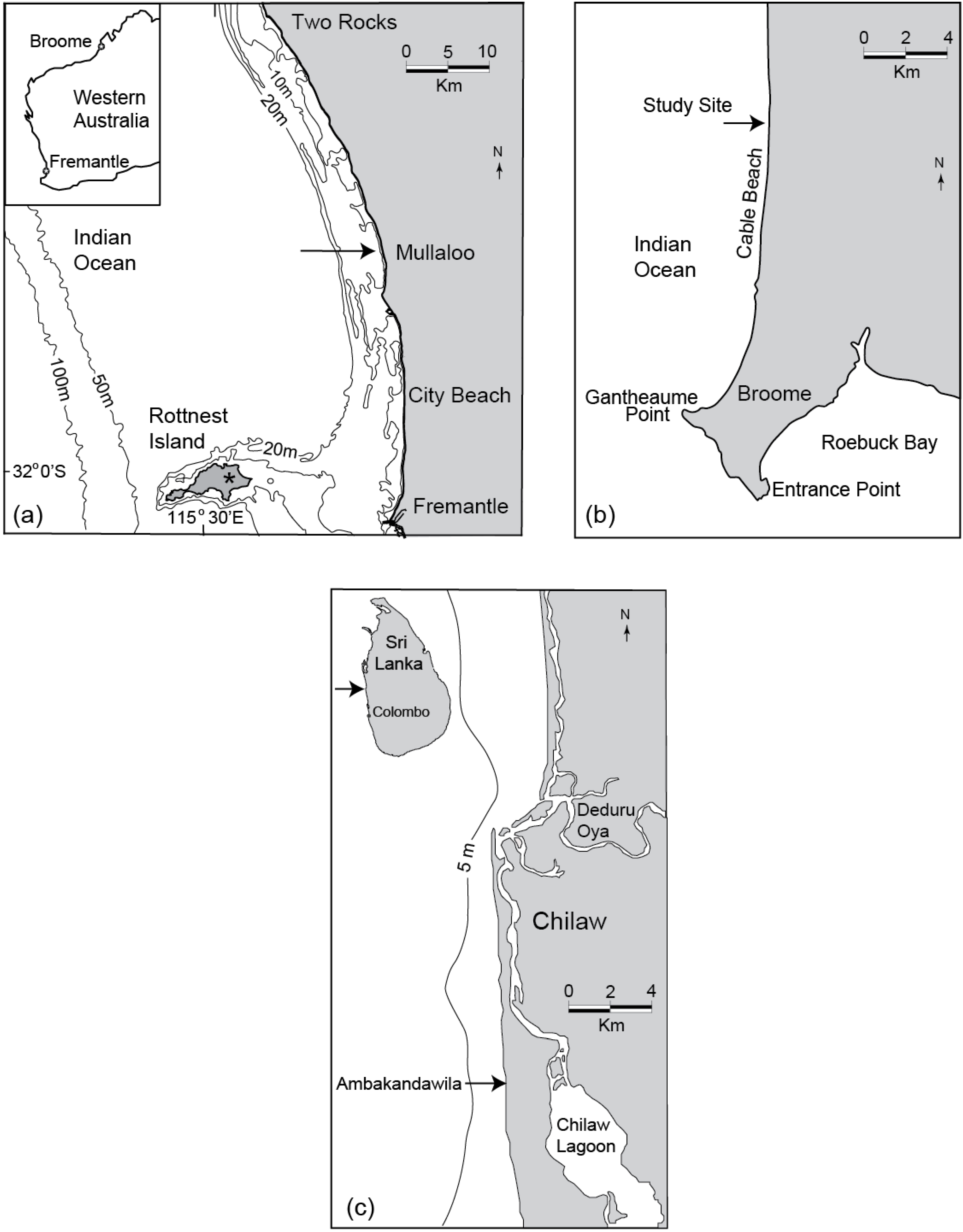
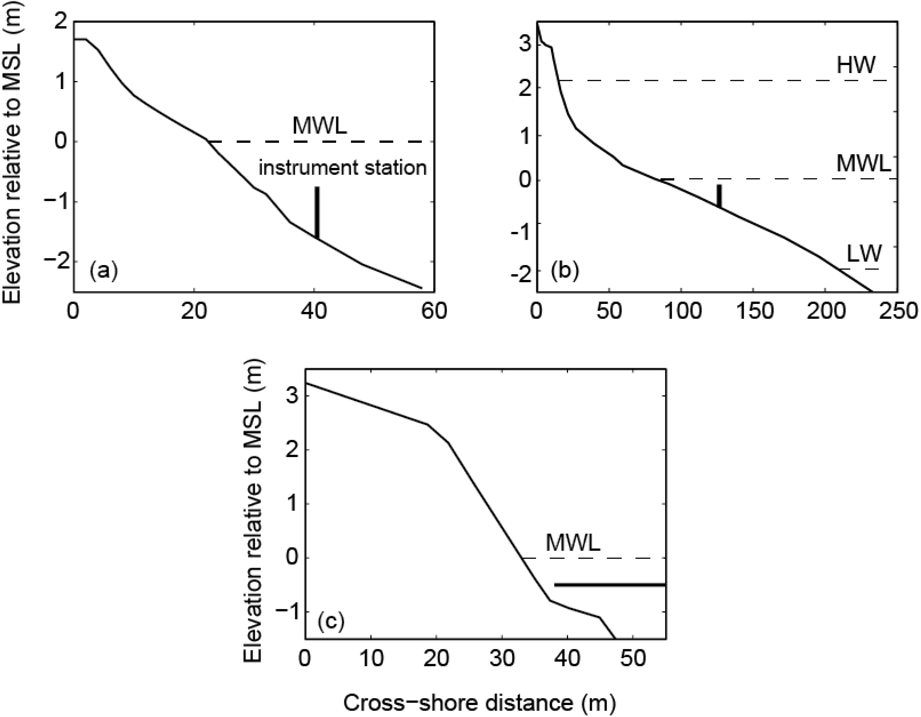
2.1. Field Sites


| Mullaloo Beach, Perth, Western Australia | Cable Beach, Broome, Western Australia | Ambakandawila Beach, Chilaw Sri Lanka | |
|---|---|---|---|
| Date of experiment | April (autumn), 1993 | August (winter), 1997 | January (summer), 1996 |
| Mean tidal range | 0.6 m | 9.8 m | 0.8 m |
| Mean wave height | 0.5–1.5 m | 0.5–1.5 m | 0.5–1.5 m |
| Peak Period | 14.9 s | 14.8 s | 14.2 s |
| Breaker type | Surging | Spilling | Surging |
| Beach morphology | Reflective, non-barred | Dissipative, non-barred | Reflective, non-barred |
| Grain size (d50) | 0.28 mm | 0.15 mm | 0.11 mm |
| Measurement locations | Close to breaker zone | Inside and outside of the breaker zone depending on tidal state | Inside and outside of the breaker zone; instrument location changed during measurement period |
| Data collection rate | 5 Hz | 5 Hz | 2 Hz |

2.2. Field Data Collection
2.3. Data Analysis Techniques
2.4. The Dean Number


3. Results
3.1. Sediment Resuspension


3.2. Cross-Shore Sediment Flux
3.2.1. Shoaling, Non-Breaking Waves over a Flat Bed


3.2.2. Temporal Variability: Tidal Cycle


3.2.3. Spatial Variability: Inside and Outside of the Surf Zone


3.2.4. Variation with the Dean Number

4. Discussion
4.1. Cross-Shore Location
4.2. Bed Ripples
4.3. Velocity Skewness (<u3>/<u2>3/2)
4.4. Dean Number (D)
5. Conclusions
- (a)
- A significant correlation between wave groups and suspended sediment concentration was observed at all of the measurement sites, confirming the well-established assumption that wave groups are more capable than incident swell waves of equal amplitude of suspending sediments. This correlation was observed in the presence and absence of ripples.
- (b)
- The direction and magnitude of suspended sediment flux varied depending on the measurement location with respect to the breaker line; however, other parameters, such as bed ripples and velocity skewness, could have influenced this.
- (c)
- At infragravity frequencies, the suspended sediment flux was mainly offshore outside of the surf zone (due to the combined action of wave groups and the group-bound long wave), while it varied inside of the surf zone. The wave groupiness factor was greater farther offshore of the surf zone and was relatively low inside of the surf zone.
- (d)
- The direction and magnitude of the suspended sediment flux inside of the breaker line changed with the breaker type.
- (e)
- Offshore suspended sediment flux due to swell waves was observed over less steep post-vortex ripples.
- (f)
- At the swell frequency band, onshore sediment flux was observed when the normalised velocity skewness was high; offshore flux was observed when the skewness was lower, but still positive, suggesting the influence of other parameters, such as ripples and grain size [28].
- (g)
- Suspended sediment flux due to swell waves was predominantly onshore when the Dean number was less than 1.67 and offshore when the Dean number was greater than 1.67. This agreed with Dean and Dalrymple’s [44] simple hypothesis, although it did not account for the influence of bed ripples or wave asymmetry.
Acknowledgments
Author Contributions
Conflicts of Interest
References
- Masselink, G.; Pattiaratchi, C. The effect of sea breeze on beach morphology, surf zone hydrodynamics and sediment resuspension. Mar. Geol. 1998, 146, 115–135. [Google Scholar] [CrossRef]
- Yates, M.L.; Guza, R.T.; O’Reilly, W.C. Equilibrium shoreline response: Observations and modeling. J. Geophys. Res. 2009, 114, C09014. [Google Scholar] [CrossRef]
- Hanson, H.; Larson, M.; Kraus, N.C. Calculation of beach change under interacting cross-shore and longshore processes. Coast. Eng. 2010, 57, 610–619. [Google Scholar] [CrossRef]
- Sternberg, R.W.; Shi, N.C.; Downing, J.P. Continuous measurements of suspended sediment. In Nearshore Sediment Transport; Seymour, R.J., Ed.; Springer: New York, NY, USA, 1989; pp. 231–257. [Google Scholar]
- Baldock, T.E.; Alsina, J.A.; Caceres, I.; Vicinanza, D.; Contestabile, P.; Power, H.; Sanchez-Arcilla, A. Large-scale experiments on beach profile evolution and surf and swash zone sediment transport induced by long waves, wave groups and random waves. Coast. Eng. 2011, 58, 214–227. [Google Scholar] [CrossRef]
- Huntley, D.A.; Hanes, D.M. Direct measurement of suspended sediment transport. In Coastal Sediments ’87, Proceedings of a Specialty Conference on Advances in Understanding of Coastal Sediment Processes, New Orleans, LA, USA, 12–14 May 1987; Kraus, N.C., Ed.; American Society of Civil Engineers: New York, NY, USA, 1987; pp. 723–737. [Google Scholar]
- Brenninkmeyer, B.M. In situ measurements of rapidly fluctuating, high sediment concentrations. Mar. Geol. 1976, 20, 117–128. [Google Scholar] [CrossRef]
- Sternberg, R.W.; Shi, N.C.; Downing, J.P. Field investigations of suspended sediment transport in the nearshore zone. In Coastal Engineering (1984), Proceedings of the International Nineteenth Coastal Engineering Conference, Houston, TX, USA, 3–7 September 1984; Edge, B.L., Ed.; American Society of Civil Engineers: New York, NY, USA, 1984; pp. 1782–1798. [Google Scholar]
- Hanes, D.M.; Huntley, D.A. Continuous measurements of suspended sand concentration in a wave dominated nearshore environment. Cont. Shelf Res. 1986, 6, 585–596. [Google Scholar] [CrossRef]
- Osborne, P.D.; Greenwood, B. Sediment suspension under waves and currents: Time scales and vertical structure. Sedimentology 1993, 40, 599–622. [Google Scholar] [CrossRef]
- Hanes, D.M. Suspension of sand due to wave groups. J. Geophys. Res. 1991, 96, 8911–8915. [Google Scholar] [CrossRef]
- Vincent, C.E.; Hanes, D.M.; Bowen, A.J. Acoustic measurements of suspended sand on the shoreface and the control of concentration by bed roughness. Mar. Geol. 1991, 96, 1–18. [Google Scholar] [CrossRef]
- Williams, J.J.; Rose, C.P.; Thorne, P.D. Role of wave groups in resuspension of sandy sediments. Mar. Geol. 2002, 183, 17–29. [Google Scholar] [CrossRef]
- Kularatne, S.; Pattiaratchi, C.B. Turbulent kinetic energy and sediment resuspension due to wave groups. Cont. Shelf Res. 2008, 28, 726–736. [Google Scholar] [CrossRef]
- Davidson, M.A.; Russell, P.E.; Huntley, D.A.; Hardisty, J. Tidal asymmetry in suspended sand transport on a macrotidal intermediate beach. Mar. Geol. 1993, 110, 333–353. [Google Scholar] [CrossRef]
- Hay, A.E.; Bowen, A.J. Coherence scales of wave-induced suspended sand concentration fluctuations. J. Geophys. Res. 1994, 99, 12749–12766. [Google Scholar] [CrossRef]
- Villard, P.V.; Osborne, P.D. Visualization of wave-induced suspension patterns over two-dimensional bedforms. Sedimentology 2002, 49, 363–378. [Google Scholar] [CrossRef]
- Doering, J.C.; Bowen, A.J. Wave-induced flow and nearshore suspended sediment. In Coastal Engineering (1988), Proceedings of the International Twenty-first Coastal Engineering Conference, Coata del Sol-Malaga, Spain, 20–25 June 1988; Edge, B.L., Ed.; American Society of Civil Engineers: New York, NY, USA, 1989; pp. 1452–1463. [Google Scholar]
- Osborne, P.D.; Greenwood, B. Frequency dependent cross-shore suspended sediment transport. 1. A non-barred shoreface. Mar. Geol. 1992, 106, 1–24. [Google Scholar] [CrossRef]
- Longuet-Higgins, M.S.; Stewart, R.W. Radiation stresses in water waves: A physical discussion, with applications. Deep Sea Res. 1964, 11, 529–562. [Google Scholar]
- Larsen, L.H. A new mechanism for seaward dispersion of midshelf sediments. Sedimentology 1982, 29, 279–283. [Google Scholar] [CrossRef]
- Shi, N.C.; Larsen, L.H. Reverse sediment transport induced by amplitude-modulated waves. Mar. Geol 1984, 54, 181–200. [Google Scholar] [CrossRef]
- Osborne, P.D.; Greenwood, B. Frequency dependent cross-shore suspended sediment transport. 2. A barred shoreface. Mar. Geol. 1992, 106, 25–51. [Google Scholar] [CrossRef]
- Aagaard, T.; Greenwood, B. Suspended sediment transport and morphological response on a dissipative beach. Cont. Shelf Res. 1995, 15, 1061–1086. [Google Scholar] [CrossRef]
- Osborne, P.D.; Vincent, C.E. Dynamics of large and small scale bedforms on a macrotidal shoreface under shoaling and breaking waves. Mar. Geol. 1993, 115, 207–226. [Google Scholar] [CrossRef]
- Osborne, P.D.; Vincent, C.E. Vertical and horizontal structure in suspended sand concentrations and wave-induced fluxes over bedforms. Mar. Geol. 1996, 131, 195–208. [Google Scholar] [CrossRef]
- Doucette, J.S. The distribution of nearshore bedforms and effects on sand suspension on low-energy, micro-tidal beaches in southwestern Australia. Mar. Geol. 2000, 165, 41–61. [Google Scholar] [CrossRef]
- Russell, P.E.; Huntley, D.A. A cross-shore transport “shape function” for high energy beaches. J. Coast. Res. 1999, 15, 198–205. [Google Scholar]
- Aagaard, T.; Nielsen, J.; Greenwood, B. Suspended sediment transport and nearshore bar formation on a shallow intermediate-state beach. Mar. Geol. 1998, 148, 203–225. [Google Scholar] [CrossRef]
- Conley, D.C.; Beach, R.A. Cross-shore sediment transport partitioning in the nearshore during a storm event. J. Geophys. Res. 2003, 108. [Google Scholar] [CrossRef]
- Pattiaratchi, C.B. Coastal tide gauge observations: Dynamic processes present in the Fremantle record. In Operational Oceanography in the 21st Century; Schiller, A., Brassington, G.B., Eds.; Springer: Heidelberg, Germany, 2011; pp. 185–202. [Google Scholar]
- Pattiaratchi, C.; Hegge, B.; Gould, J.; Eliot, I. Impact of sea-breeze activity on nearshore and foreshore processes in southwestern Australia. Cont. Shelf Res. 1997, 17, 1539–1560. [Google Scholar] [CrossRef]
- Masselink, G.; Pattiaratchi, C.B. Seasonal changes in beach morphology along the sheltered coastline of Perth, Western Australia. Mar. Geol. 2001, 172, 243–263. [Google Scholar] [CrossRef]
- Masselink, G.; Pattiaratchi, C. Tidal asymmetry in sediment resuspension on a macrotidal beach in northwestern Australia. Mar. Geol. 2000, 163, 257–274. [Google Scholar] [CrossRef]
- Pattiaratchi, C.; Masselink, G.; Wikramanayake, N. Sea breeze effects on coastal processes. In Proceedings of the Fifth International Conference on Coastal and Port Engineering in Developing Countries (COPEDEC V), Cape Town, South Africa, 16–17 April 1999; Council for Scientific and Industrial Research: Cape Town, South Africa, 1999; pp. 37–48. [Google Scholar]
- Foote, Y.; Russell, P.E.; Huntley, D.A.; Sims, P. Energetics prediction of frequency-dependent suspended sand transport rates on a macrotidal beach. Earth Surf. Process. Landf. 1998, 23, 927–941. [Google Scholar] [CrossRef]
- Ludwig, K.A.; Hanes, D.M. A laboratory evaluation of optical backscatterance suspended solids sensors exposed to sand-mud mixtures. Mar. Geol. 1990, 94, 173–179. [Google Scholar] [CrossRef]
- Bendat, J.S.; Piersol, A.G. Random Data: Analysis and Measurement Procedures; Wiley-Interscience: New York, NY, USA, 1986. [Google Scholar]
- Jenkins, G.M.; Watts, D.G. Spectral Analysis and Its Applications; Holden-Day: San Francisco, CA, USA, 1968; p. 525. [Google Scholar]
- List, J.H. Wave groupiness variations in the nearshore. Coast. Eng. 1991, 15, 475–496. [Google Scholar] [CrossRef]
- Dean, R.G. Heuristic models of sand transport in the surf zone. In Proceedings of the Conference on Engineering Dynamics in the Surf Zone; American Society of Civil Engineers: New York, NY, USA, 1973; pp. 208–214. [Google Scholar]
- Dean, R.G.; Dalrymple, R.A. Coastal Processes with Engineering Applications; Cambridge University Press: New York, NY, USA, 2002; p. 475. [Google Scholar]
- Clifton, H.E.; Dingler, J.R. Wave-formed structures and paleoenvironmental reconstruction. Mar. Geol. 1984, 60, 165–198. [Google Scholar] [CrossRef]
- Nielsen, P. Coastal Bottom Boundary Layers and Sediment Transport; Advanced Series on Ocean Engineering; World Scientific: Singapore, Singapore, 1992; Volume 4, p. 324. [Google Scholar]
- Elgar, S.; Guza, R.T.; Freilich, M.H. Eulerian measurements of horizontal accelerations in shoaling gravity waves. J. Geophys. Res. 1988, 93, 9261–9269. [Google Scholar] [CrossRef]
- Inman, D.L.; Bowen, A.J. Flume experiments on sand transport by waves and currents. In Coastal Engineering (1962), Proceedings of the eighth International Coastal Engineering Conference, Mexico City, Mexico, 26–29 November 1962; Edge, B.L., Ed.; American Society of Civil Engineers: New York, NY, USA, 1963; pp. 137–150. [Google Scholar]
- Brander, R.W.; Greenwood, B. Bedform roughness and the re-suspension and transport of sand under shoaling and breaking waves: A field study. In Proceedings of Canadian Coastal Conference, Vancouver, BC, Canada, 4–7 May 1993; Coastal Zone Canada Association: Ottawa, Canada, 1993; pp. 587–599. [Google Scholar]
- Kularatne, S.R.; Pattiaratchi, C.B. Numerical model study of cross-shore suspended sediment flux in the frequency domain. Coast. Eng. J. 2014. in review. [Google Scholar]
© 2014 by the authors; licensee MDPI, Basel, Switzerland. This article is an open access article distributed under the terms and conditions of the Creative Commons Attribution license (http://creativecommons.org/licenses/by/3.0/).
Share and Cite
Kularatne, S.; Pattiaratchi, C. The Role of Infragravity Waves in Near-Bed Cross-Shore Sediment Flux in the Breaker Zone. J. Mar. Sci. Eng. 2014, 2, 568-592. https://doi.org/10.3390/jmse2030568
Kularatne S, Pattiaratchi C. The Role of Infragravity Waves in Near-Bed Cross-Shore Sediment Flux in the Breaker Zone. Journal of Marine Science and Engineering. 2014; 2(3):568-592. https://doi.org/10.3390/jmse2030568
Chicago/Turabian StyleKularatne, Samantha, and Charitha Pattiaratchi. 2014. "The Role of Infragravity Waves in Near-Bed Cross-Shore Sediment Flux in the Breaker Zone" Journal of Marine Science and Engineering 2, no. 3: 568-592. https://doi.org/10.3390/jmse2030568
APA StyleKularatne, S., & Pattiaratchi, C. (2014). The Role of Infragravity Waves in Near-Bed Cross-Shore Sediment Flux in the Breaker Zone. Journal of Marine Science and Engineering, 2(3), 568-592. https://doi.org/10.3390/jmse2030568