On Peak Mooring Loads and the Influence of Environmental Conditions for Marine Energy Converters

Abstract

Mooring systems are among the most critical sub-systems for floating marine energy converters (MEC). In particular, the occurrence of peak mooring loads on MEC mooring systems must be carefully evaluated in order to ensure a robust and efficient mooring design. This understanding can be gained through long-term field test measurement campaigns, providing mooring and environmental data for a wide range of conditions. This paper draws on mooring tensions and environmental conditions that have been recorded (1) for several months during the demonstration of an MEC device and (2) over a period of 18 months at a mooring test facility. Both systems were installed in a shallow water depth (45 m and 30 m, respectively) using compliant multi-leg catenary mooring systems. A methodology has been developed to detect peak mooring loads and to relate them to the associated sea states for further investigation. Results indicate that peak mooring loads did not occur for the sea states on the external contour line of the measured sea states, but for the sea states inside the scatter diagram. This result is attributed to the short-term variability associated with the maximum mooring load for the given sea state parameters. During the identified sea states, MEC devices may not be in survival mode, and thus, the power take-off (PTO) and ancillary systems may be prone to damage. In addition, repeated high peak loads will significantly contribute to mooring line fatigue. Consequently, considering sea states inside the scatter diagram during the MEC mooring design potentially yields a more cost-effective mooring system. As such, the presented methodology contributes to the continuous development of specific MEC mooring systems.

1. Introduction

The use of renewable energy has been increasing over the last 40 years and will keep increasing because of climate change concerns, the rise of the price of fossil resources, the need for energy independence and growing energy demand. Marine renewable energy has the potential to provide a significant amount of renewable energy.

The main challenge for the development of marine renewable energy is to be cost effective. The predicted electricity generating costs of marine energy converters (MEC) have been significantly decreasing in the last twenty years [1]. In order to harvest the most energetic sea states, allowing increased competitiveness, systems have evolved from onshore to offshore systems and, consequently, from fixed to floating structures. Floating MECs require mooring systems, which are essential for the MEC’s survival. However, the cost of the mooring systems is much more critical for an MEC project than for an oil and gas project. In the example given by Fitzgerald [2], for an oil and gas project, the mooring costs represent less than 2% of the lifetime costs, while the mooring costs are equal to 18% of the wave energy project lifetime costs.

MECs have specific requirements in terms of mooring systems. Large offshore structures have their resonant frequencies significantly different from the wave frequency (WF) in order to avoid large resonant effects. On the contrary, most of the MEC devices need to be designed for resonant WF to produce energy [3]. The other MEC devices that do not need to be designed for resonant WF may also have physical properties (length, mass, etc.) that do not allow avoiding their resonant frequency to be significantly different from WF excitations. Regarding wave energy converter (WEC) devices, whilst for some WEC devices, the power take-off (PTO) system is directly coupled to the mooring system, other device design principles have their PTO system acting against a moored “superstructure”; for example, the Wavedragon; the superstructure would typically be designed to be away from the excitation frequency [3].

Prototype testing and full-scale testing of MEC devices are now being conducted. Field tests give insight into the behaviour of the MEC devices in real sea conditions. Measuring the mooring loads and the environmental conditions—wave and current, if available—of two mooring systems for several months, a methodology has been developed to identify the peak mooring loads and to present the mooring load measurements—their amplitude and percentage of occurrences—and their associated environmental conditions.

This paper is divided into seven sections, including the Introduction. The field measurements that have been used for this study are described in Section 2. The methodology to detect peak mooring load is outlined in Section 3. The assessment of the general environmental conditions and of the environmental conditions associated with peak mooring load is explained in Section 4. Results are presented in Section 5 and discussed in Section 6, followed by a conclusion in Section 7.

2. Mooring Sea Trial Facilities

Two facilities were used to gather data for this study: the South West Mooring Test Facility (SWMTF) and the Falmouth Bay Test Site (FaBTest), where the Fred Olsen Bolt-2 Lifesaver wave energy device was installed. These two facilities are located in the southwest of the U.K., less than three nautical miles (~5 km) apart on the South Cornish coast (Figure 1).

2.1. South West Mooring Test Facility

The SWMTF is installed in Falmouth Bay, Cornwall, U.K. This facility has been built to conduct long-term sea trials for moorings of MEC devices. The location was chosen to provide a location near a port and with wave conditions with a one-third scale to the Wave Hub site. The water depth at this site is between 27 m (Lowest Astronomical Tide: LAT) and 32.4 m (Highest Astronomical Tide: HAT). The deployment position of the buoy is 50°47.5′ N, 5°2.85′ W.

This facility has been previously described by Harnois et al. [4] and Johanning et al. [5]. The measurements of this facility have also been used by Thies et al. [6], for mooring line fatigue evaluation. The instruments used for this paper are described below, and their properties are presented in

Table 1. Summary of instrumentation at SWMTF.

Sensor	Parameter	Sample Frequency (Hz)	Data Sample Size
Teledyne RDI Workhorse Sentinel ADCP	Surface elevation and water current velocities converted into: wave: HS (m), TP (s), DP (deg); current: mean current magnitude CMag (m/s) and direction CDir (deg) along the water column (0.5-m bins)	2 Hz	1024 s
Axial load cells	Mooring loads: time series of loads (kN)	20 Hz	10 min

. A tank test of this buoy has also been conducted by Harnois et al. [7].

An instrumented surface buoy of 3250 kg and a 2.9-m float diameter (Figure 2a) was equipped with conventional axial load cells (Figure 2b) to record mooring load data at 20 Hz. For the test presented in this paper, this buoy was moored with a three leg combined (hybrid) chain fibre rope mooring system arranged as drawn in Figure 2c. The mooring legs combined chains and nylon rope as detailed in

Table 2. Summary of mooring line components at SWMTF.

	Mooring at SWMTF (from Seabed to Surface)
Type of Legs	Catenary
Number of equally-spread lines	3
Anchor type	Drag embedment anchor
Total length of each leg (including sensors and connections)	63 m
Length of the line in the water column	~38 m
Static tension	~3 kN
Weight to avoid large excursion or vertical mooring load on the anchor	4 m of DN32 stud link chain, 22 kg/m in air
No contact of the nylon rope with the seabed	36 m of DN24 open link chain, 11 kg/m in air
Nylon rope to provide compliance	20 m of 44-mm nylon rope, 1.2 kg/m in air
Protection of the top end of the nylon rope and mooring load measurement	Chain and load cells
Buoy	3.25-tonne buoy

. The heave, roll and pitch natural periods are between 2 and 2.5 s.

The data were continuously recorded and saved every 10 min. The values for the average, maximum and standard deviation of the mooring load during each 10-min interval were calculated and saved separately.

A Workhorse Sentinel Acoustic Doppler current profiler (ADCP) (Figure 2d) was equipped with four inclined beams to record wave and current data at 2 Hz, with a bin height of s = 0.5 m [8]. The ADCP is installed on the seabed 25 m towards the southeast direction with respect to the buoy equilibrium position as indicated in Figure 2c. The data were continuously recorded and saved every 17.067 min (2048 points). After the recovery of the ADCP, which is retrieved approximately every three months, the data were processed using WavesMon, a software package provided by Teledyne RDI to obtain data for several wave and current parameters, such as the significant wave height H_S, the peak period T_P, time-averaged current magnitudes for all bins in a vertical water column C_Mag, their corresponding current directions (current heading) C_Dir and the water depth h for each 17.067-min file.

2.2. FaBTest: Bolt-2 Lifesaver Device

The “Bolt-2 Lifesaver” wave energy device [9] has been installed at the Falmouth Bay test site (FaBTest) [10], Cornwall, U.K. The FaBTest site is a demonstration facility that enables device developers to test components, concepts or full-scale devices in a moderate wave climate with excellent access to nearby port infrastructure. The aim of the Technology Strategy Board (TSB) project was to conduct sea trials at full scale, before a deployment in less sheltered conditions. The water depth at this site is between 45 m (LAT) and 51 m (HAT). The deployment position of the floating structure was 50°6.0402′ N, 4°59.6455′ W. The instruments used for this paper are described below, and their properties are presented in

Table 3. Summary of the instrumentation at the Bolt-2 LifeSaver installation.

Sensor	Parameter	Sample Frequency (Hz)	Data Sample Size
FUGRO Oceanor Seawatch mini II directional wave buoy	HS,TP and DP	2	30 min
Axial load cells: Strainstall 5395 Underwater load shackles	Time series of mooring loads (tonnes)	200	Up to 20 min

.

An instrumented surface annulus buoy (Figure 3a) of 40 tonnes and a 10-m inner diameter, a 16-m outer diameter and a 1-m height was equipped with five conventional axial load cells (Figure 3b) to record mooring load data at 200 Hz. This buoy was moored with a five leg catenary mooring system installed as shown in Figure 3c. The mooring legs combined chains and nylon rope as described in

Table 4. Summary of the mooring line components at the Bolt-2 LifeSaver installation.

	Mooring at Fred Olsen Device (from Seabed to Surface)
Type of Legs	Catenary
Number of equally-spread lines	5
Anchor type	Drag embedment anchor
Total length of each leg (including sensors and connections)	113 to 153 m
Length of the line in the water column	~91 m
Static tension	~7.5 kN
Weight to avoid large excursion or vertical mooring load on the anchor	line 1 to 5: 70/80/40/40/70 m DN60 stud link chain, Grade 1 79 kg/m in air
No contact of the nylon rope with the seabed	38 m of DN36 open link chain, Grade 2 26 kg/m in air
Nylon rope to provide compliance	32 m of 64 mm nylon braid line rope
	2.5 kg/m in air
Protection of the top end of the nylon rope	3 m of DN36 open link chain, Grade 2 26 kg/m in air
Buoy	~40-tonne buoy

. Data were recorded and saved in files containing a maximum of 20 min of data (240,000 data points); this was not on a continuous basis, but based on the discretion of the wave energy developer. The average, maximum and standard deviation of the mooring load during each record period were calculated and saved in a separate file.

A Seawatch mini II directional wave buoy (Figure 3d) was used to record wave data at 2 Hz [11,12]. The wave buoy was installed at 334 m from the Bolt-2 Lifesaver device (Figure 3c). Data were continuously recorded, then processed at the buoy every 30 min by the on-board software WaveSense. The processed statistical wave data, such as H_S and T_P, were saved.

3. Methodology to Detect Peak Mooring Loads

A methodology has been developed to isolate peak mooring loads. Peak mooring loads are defined as sudden mooring loads with a large amplitude.

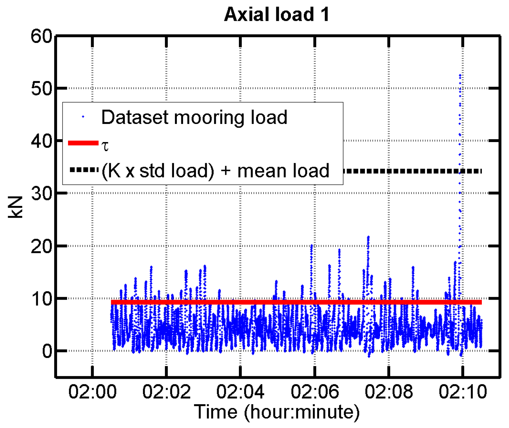
During the deployment, time series of mooring load data were measured with inline load cells at 20 Hz (SWMTF) and 200 Hz (Bolt-2 Lifesaver). The processing of mooring load data started with a quality check applied on the mooring load data assessing possible drift or offset for these data, as described by Thies et al. [6].

An example of the time series of mooring loads at SWMTF is presented in Figure 4. A sudden increase in tension to 53 kN is observed between 9 and 10 min, and the standard deviation of the load is large during the whole dataset.

A minimum threshold τ and a peak mooring load factor K are introduced to determine if the datasets contain peak mooring loads. τ is compared to the maximum mooring load of the dataset while K is compared to the standard score of the maximum S_max of the dataset. The minimum threshold τ is used to identify mooring loads with a sufficiently large amplitude, while the peak mooring load factor K is introduced to isolate datasets containing sharp mooring loads. K basically checks that the peak load is the result of a dynamic behaviour and not from an increase in load due to slow second order motion. The calculation of the standard score of the maximum (Equation (1)) gives the difference between the maximum and the mean per unit standard deviation and allows the comparison of: (i) the dynamic part of the load (the amplitude of the maximum mooring load minus the mean mooring load); and (ii) of the spreading of the mooring loads in the selected dataset.

$$S_{\max }(x)=\frac{\max (x)-\overline{x}}{{\sigma }_x}$$

(1)

x is the dataset of the mooring load, S_max the standard score of the maximum, $\overline{x}$ the mean of x and ${\sigma }_x$ the standard deviation of x.

An increase in load due to slow second order motion would result in an increase in the standard deviation of mooring load and a decrease in the standard score of the maximum mooring load.

S_max assesses the non-linearity of mooring loads. This non-linearity can be caused by:

• Geometric non-linearity that is associated with changes in the shape of the mooring line caused by vertical force components;
• Non-linear stretching of synthetic ropes;
• Non-linear seabed friction;
• Non-linear drag of the mooring line, which may cause snap loads.

The larger the K and τ values, the less datasets of mooring loads are identified as containing peak mooring loads, as shown in the example in

Table 5. Example of the percentage of occurrences of SWMTF datasets considered as containing peak mooring loads on line 1 for different values of τ and K. The joint percentage of occurrences (JPOs) of the τ\K combinations corresponding to the numbers in italics have been plotted in Figure 15.

τ\K	0	2.5	5	7.5	10
0 kN	100.00%	99.98%	14.56%	0.40%	0.02%
7.5 kN	13.29%	13.29%	6.45%	0.32%	0.01%
10 kN	5.00%	5.00%	3.38%	0.27%	0.01%
12.5 kN	2.09%	2.09%	1.64%	0.18%	0.01%
20 kN	0.25%	0.25%	0.25%	0.07%	0.01%
30 kN	0.04%	0.04%	0.04%	0.02%	0.01%
40 kN	0.01%	0.01%	0.01%	0.01%	0.01%
50 kN	0.01%	0.01%	0.01%	0.01%	0.01%

. This example shows which percentage of datasets is defined as containing peak mooring loads on mooring line 1 at SWMTF. For example, if τ is set to 0 kN and K to zero, this means that all datasets are defined as containing peak mooring loads. If τ is set to 10 kN and K to 7.5, this means that 0.27% of the datasets are defined as containing peak mooring loads. A mooring system with a high number of mooring lines or in a calm environment will be less likely to observe peak mooring loads at a similar mooring load factor and threshold value. As a consequence, τ and K have to be chosen depending on the environmental conditions and mooring configuration (in particular, the number of mooring lines and mooring compliance). In addition, the severity of selected peak mooring loads also needs to be defined. For this paper, τ was chosen equal to three times the overall mean load on all mooring lines at both installations. This value is equal to 9.32 kN at SWMTF and 35.33 kN at the Bolt-2 Lifesaver mooring. K was chosen equal to 7.5 at both installations. These choices allow the selection of a sufficient number of peak mooring loads for further investigations.

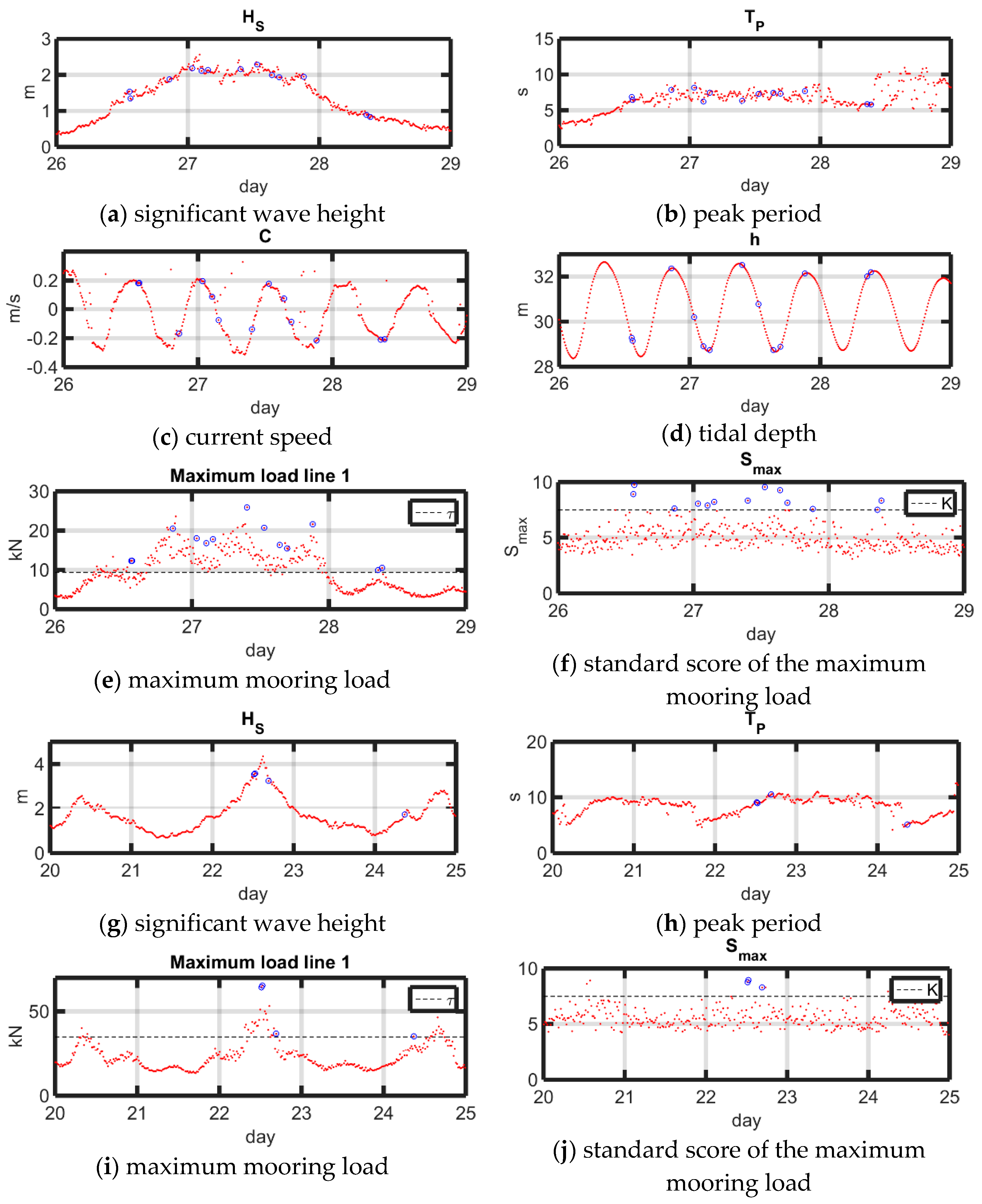
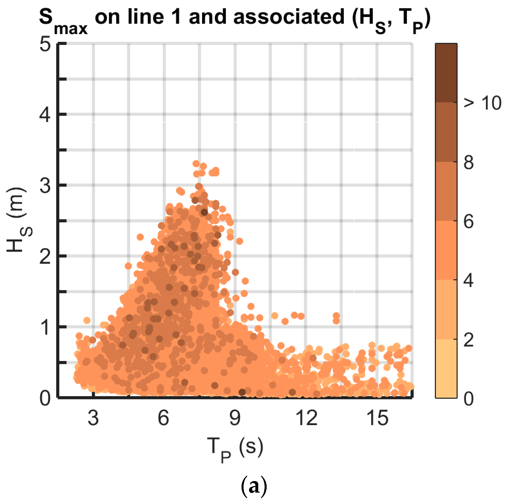
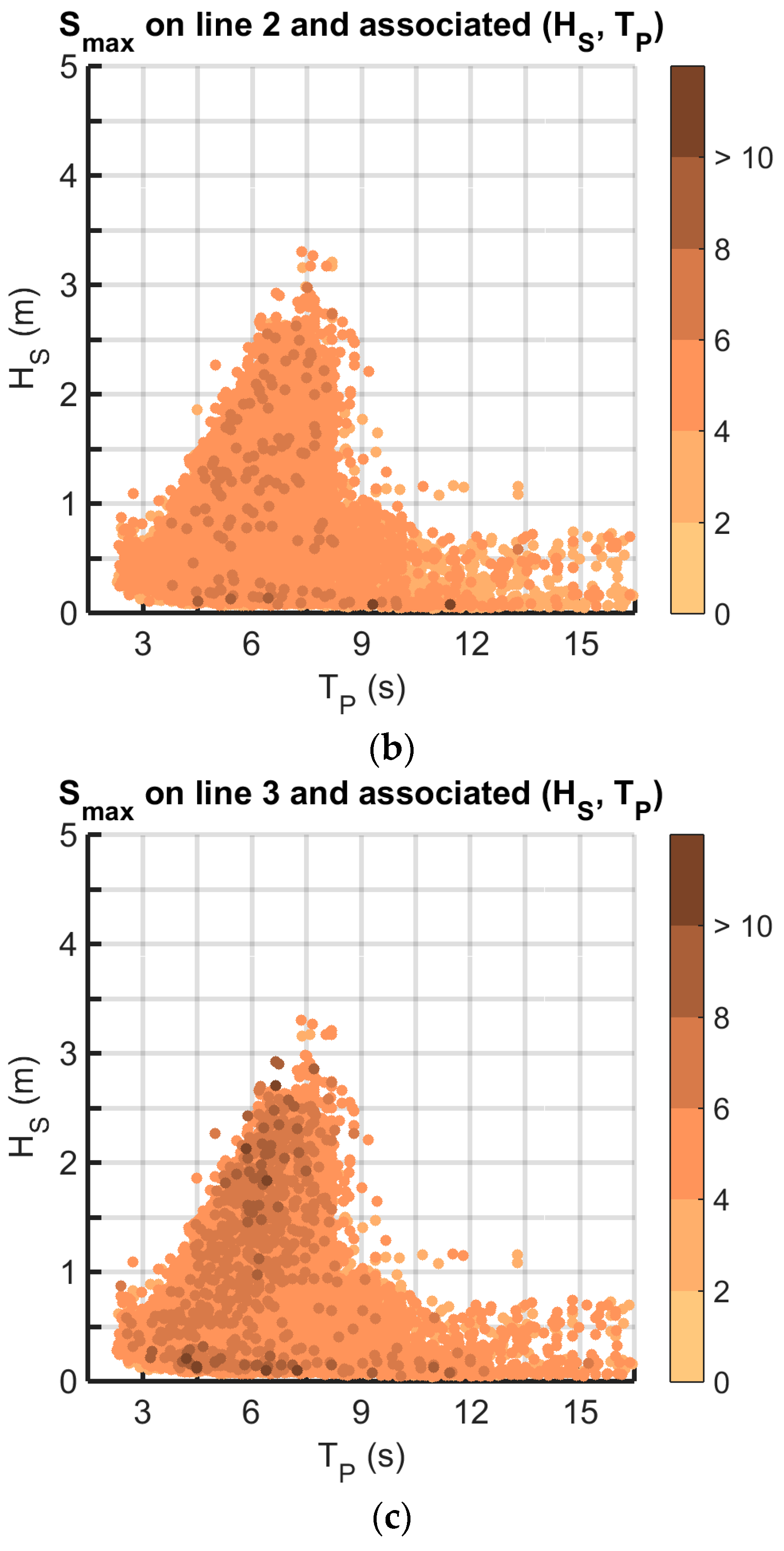
For each dataset of the time series of mooring load and for each mooring line, the standard score of the maximum is calculated and the maximum mooring load is considered. Figure 5a–f shows an example of the standard score and maximum load at SWMTF on mooring line 1 for several days, as well as the corresponding environmental conditions. Similarly, Figure 5g–j shows an example of H_S, T_P, maximum load and standard score and maximum load at the Bolt-2 LifeSaver on mooring line 1. In both cases, if the standard score and the maximum value are higher than K and τ, respectively, then a peak mooring load is detected and indicated by a blue circle. Additionally, the environmental parameters occurring at this time are recorded. This methodology is repeated on all mooring lines, applying the same mooring load factor K and threshold value τ.

4. Environmental Conditions Associated with Peak Mooring Loads

The environmental conditions recorded at the site are compared to the environmental conditions associated with peak mooring loads. In order to compare these data, the environmental conditions at the test site are initially assessed, and then, the ones associated with peak mooring loads are examined.

4.1. Assessment of the Site Environmental Conditions

In order to identify the range of sea states occurring at a site and the percentage of occurrences of these sea states during a sea trial, scatter diagrams are built.

A scatter diagram is obtained by classifying into different ranges and then counting for each range the number of occurrences of two environmental parameters, such as H_S and T_P, obtained by wave measurement or hindcast. This method is shown in Equation (2). The minimum values x₀ and y₀, bin sizes x_bin and y_bin and numbers of bins i and j are chosen to include all recorded sea states and to find a compromise between the resolution and the population of the bins.

$$SD{(x,y)}_{i,j}={\displaystyle \sum _{k=1}^{nb\_data}\langle \begin{array}{c}{x}_0+(i-1)x_{bin}\le x_k<x_0+i{x}_{bin}\\ and\\ y_0+(j-1)y_{bin}\le y_k<y_0+j{y}_{bin}\end{array}\rangle }$$

(2)

with SD as the scatter diagram and x_k and y_k the couple describing the environmental conditions for a given sea state k.

If for a given i, j and k both conditions $x_0+(i-1)x_{bin}\le x_k<x_0+i{x}_{bin}$ and $y_0+(j-1)y_{bin}\le y_k<y_0+j{y}_{bin}$ are gathered, then the value between the bracket is equal to one, else it is equal to zero.

In order to identify which sea states have been more frequent during a sea trial, the joint percentage of occurrences (JPOs) of each pair of environmental conditions is calculated by dividing the scatter diagram by the sum of all of its values (Equation (3)).

$$JPO{(x,y)}_{i,j}=\frac{SD{(x,y)}_{i,j}}{{\displaystyle \sum _{i,j}SD{(x,y)}_{i,j}}}=\frac{SD{(x,y)}_{i,j}}{nb\_data}=\frac{{\displaystyle \sum _{k=1}^{nb\_data}\langle \begin{array}{c}{x}_0+(i-1)x_{bin}\le x_k<x_0+i{x}_{bin}\\ and\\ y+(j-1)y_{bin}\le y_k<y_0+j{y}_{bin}\end{array}\rangle }}{nb\_data}$$

(3)

with JPO as the joint percentage of occurrences.

The environmental conditions considered in this paper are the wave conditions assessed with the significant wave height H_S, the peak period T_P and, if available, the tidal conditions assessed with the current velocity C and the tidal varying water depth h.

In order to assess H_S and T_P, time series of the surface elevation were recorded over a period of 17.067 min (1024 s) (SWMTF) and 30 min (FaBTest) with a measurement rate of 2 Hz. The wave statistical parameters H_S and T_P were calculated by the firmware packages provided with the wave sensors, and a quality control was applied to remove spikes, extended constant values or instrument noise following EquiMar D2.2 [13] recommendations. Sea conditions are considered stationary and the duration of the measurement sufficient to estimate the wave parameters.

At the SWMTF, time-averaged current magnitude C_Mag and direction C_Dir were additionally calculated by the ADCP manufacturer firmware WavesMon at a number of bins distributed regularly through the water column (every 0.5 m) over a period of 17.067 min. It should be noted that a surface layer, with a thickness of 5%–15% of the total water column, can be observed, as shown for example in Figure 6. In this surface layer, measurements are compromised by sidelobe reflections of the acoustic beams as discussed by RDI [14]. The maximum current magnitude C_{Mag_max} is evaluated in the bins below the surface layer. The current direction C_{Dir_max} is the direction measured at the bin of maximum current magnitude. Because the tidal flow has two opposite directions, the current velocity C is introduced in Equation (4) to summarise the magnitude and direction in a single variable.

$$C=C_{Mag\_\max }\times \cos \left[C_{Dir\_\max }-\overline{C_{Dir\_ebb}}\right]$$

(4)

with $\overline{C_{Dir\_ebb}}$ the mean ebb direction during the whole deployment.

The wave and tidal data were interpolated to provide data when mooring load data measurements were available. An example of interpolated wave parameters H_S and T_P, tidal parameters C and h and associated maximum mooring loads for the SWMTF and Bolt-2 Lifesaver installation is shown in Figure 5a–f and Figure 5g–j, respectively.

The H_S and T_P wave measurements are arranged in a 10 × 10 scatter diagram. Figure 7a is an example of such a scatter diagram. The corresponding matrix of JPO is calculated for each H_S and T_P pair in Figure 7b following Equation (5).

$$JPO{(H_S,T_P)}_{i,j}=\frac{{\displaystyle \sum _{k=1}^{nb\_data}\langle \begin{array}{c}{H}_S{}_0+(i-1)H_S{}_{bin}\le H_S{}_k<H_S{}_0+i{H}_S{}_{bin}\\ and\\ T_P{}_0+(j-1)T_P{}_{bin}\le T_P{}_k<T_P{}_0+j{T}_P{}_{bin}\end{array}\rangle }}{nb\_data}$$

(5)

with H_{S k} and T_{P k} the wave conditions at a given time, H_S0 and T_P0 the minimum wave conditions considered and H_{S bin} and T_{P bin} the bin size. For all wave scatter diagrams presented in this document, the values of H_S between 0 and 5 m were considered, with bins of 0.5 m, and the values of T_P between 1.5 s and 16.5 s with bins of 1.5 s, which include all recorded sea states and provide a good compromise between the resolution and the population of the bins.

The joint percentage of occurrence matrix is then used to draw contour lines, as shown in Figure 7c, with linear interpolation used to smooth the contour lines. These contour lines show the limit between the cases that occur and the ones that did not occur. Linear interpolation is used to plot a line between a case that occurs and a case that did not occur.

The usage of multiple contour lines allows the separation of environmental condition by percentage of occurrences. For example, a point in Figure 7c between a 3% and 6% curve means that between 3% and 6% of the recorded wave conditions were occurring in this range of occurrences of the H_S and T_P values. These contour lines should not be confused with the x-year return period contour lines as defined by the Det Norske Veritas standard DNV-OS-E301 [15]. The contour lines defined in this paper and used in the following are based on measurements and show sea states that occurred a similar number of times during a sea trial, while contour lines used for the mooring design are based on probability models and show points with the same probability of occurrence.

A similar methodology is followed for the calculation of the joint percentage of occurrences of tidal conditions, as shown in Equation (6):

$$JPO{(C,h)}_{i,j}=\frac{{\displaystyle \sum _{meas=1}^{nb\_data}\left[\begin{array}{c}{C}_0+(i-1)C_{bin}\le C_k<C_0+i{C}_{bin}\\ and\\ h_0+(j-1)h_{bin}\le h_k<h_0+j{h}_{bin}\end{array}\right]}}{nb\_data}$$

(6)

with h_k and C_k the tidal conditions at a given time, h₀ and C₀ the minimum tidal conditions and h_bin and C_bin the bin size. For all tidal diagrams considered in this document, the values of C between −0.6 and 0.6 m/s were considered, with bins of 0.12 m/s, and the values of h between 27 m and 34 s, with bins of 0.7 m.

4.2. Analysis of Environmental Conditions Associated with Peak Mooring Loads

The joint percentages of occurrences of environmental conditions associated with peak mooring loads JPO(H_{S peak}, T_{P peak}) and JPO(C_peak, h_peak) (if available) are calculated. Multi-contour plots are drawn to summarise these results. These plots indicate which wave or tidal conditions were more frequently associated with peak mooring loads. These JPOs need to be compared to the joint percentages of occurrence of general environmental conditions JPO(H_S, T_P) and JPO(C, h). For this purpose, the external contour line of the H_S and T_P JPO plot, which is the line between the observed occurrence and the absence of occurrence of a given sea state, is added to the plot of the joint percentage of occurrence of H_{S peak} and T_{P peak} (black dotted line). A similar line is added to the tidal condition plot.

5. Field Test Results

In this section, the key results of the assessment of environmental conditions associated with peak mooring load conditions are presented for the SWMTF and for the Bolt-2 Lifesaver installation. Firstly, the general environmental conditions are assessed at both sites, by plotting the contours of the joint percentage of occurrences of the measured general environmental conditions. Secondly, peak mooring loads are detected, and the contours of the joint percentage of occurrences of the environmental conditions associated with peak mooring loads are plotted. To conclude, both contour plots are compared.

5.1. South West Mooring Test Facility

The parameters H_S, T_P, C, h and the mean, max and standard deviation of mooring load data have been collected, corrected and interpolated, and an example of the data is shown in Figure 5a–f. The data used for this analysis were recorded continuously between 16 September 2010 and 27 January 2011, for a total period of 133 days. Some datasets were removed due to a lack of wave data available at the same time.

5.1.1. Environment

The contour plot of the joint percentage of occurrences of H_S and T_P is shown in Figure 8a. The interpolated sea states were classified into 41 sea state ranges. The sea states that occurred more than 7.5% of the time during the period of measurement were for H_S below 1 m and T_P between 4 and 7 s. The maximum measured H_S was below 4 m.

The contour plot of the joint percentage of occurrences of h and C is shown in Figure 8b. The measured and interpolated current parameters were classified into 54 tidal combinations. Tidal conditions with occurrences higher than 7.5% occurred for h between 31.4 and 31.9 m and C between −0.1 and 0 m/s.

5.1.2. Peak Mooring Loads

The amplitude of the maximum load recorded on each mooring line, as well as the associated wave conditions are plotted in Figure 9a–c. Figure 9a,c indicates that only one dataset of mooring load on line 1 and line 3, respectively, had a maximum load over 50 kN. This maximum load occurred for two distinct sea states. In both cases, this maximum occurs for H_S approximately equal to 2.5 m and T_P to 7 s. Figure 9a,c also indicates that there were more datasets with the maximum over 30 kN occurring on mooring line 3 than on mooring line 1. Figure 9b shows that all mooring loads on line 2 were below 20 kN. Figure 9a–c also shows that the maximum mooring loads are generally higher for high H_S values.

The standard score of the maximum S_max recorded on each mooring line, as well as the associated wave conditions are plotted in Figure 10a–c. These figures indicate that high values of S_max can occur for any sea state. Higher values of S_max are achieved on lines 1 and 3 than on line 2.

The combination of the maximum mooring load and standard score of the maximum S_max was used to detect peak mooring loads.

Table 6. Number/percentage of detected peak mooring loads for the SWMTF and the Bolt-2 Lifesaver device.

SWMTF		Bolt-2 LifeSaver
line (Orientation °)	Number of Peak Loads/Percentage of Datasets Containing Peak Loads	line (Orientation °)	Number of Peak Loads/Percentage of Datasets Containing Peak Loads
line 1 (185°)	55/0.29%	line 1 (136°)	23/0.47%
line 2 (305°)	1/0.01%	line 2 (64°)	1/0.02%
line 3 (65°)	73/0.39%	line 3 (352°)	0/0%
		line 4 (280°)	1/0.02%
		line 5 (208°)	11/0.23%
Total number of 10-min datasets with wave data available	18,837	Total number of datasets after correction and with wave data available at the same time	4878
Total number of 10-min datasets with 90° < DP < 150°	8878/47%	Total number of datasets with 120° < Dmean < 150°	745/15%
Total number of 10-min datasets with 150° < DP < 210°	9052/48%	Total number of datasets with 180° < Dmean < 210°	2060/42%

shows that only one peak mooring load occurrence was observed in mooring line 2, while 55 and 73 occurrences were identified on lines 1 and 3, respectively. This can be explained by the fact that mooring line 2 is not facing the wave direction (Figure 2c) and that the waves were evenly distributed between their two predominant directions.

Figure 11a–c shows the joint percentage of occurrences of wave conditions associated with peak mooring loads on each mooring line. Peak mooring loads occurred for 13, 1 and 12 different ranges of sea states for lines 1, 2 and 3, respectively. Most of the measured peak mooring loads were observed on line 1 (Figure 11a) and on line 3 (Figure 11c) for ranges of H_S and T_P inside the scatter diagram. The number of peak mooring loads detected on mooring line 2 is too low to include it in any conclusions.

The total number of datasets is reminded in the last three rows, as well as the number of datasets associated with a range of wave directions.

Figure 11d–f shows the joint percentage of occurrences of tidal conditions associated with peak mooring loads on all mooring lines. Peak mooring loads occurred for 22, 1 and 28 different ranges of sea states for lines 1, 2 and 3, respectively. More than 7.5% of the observed peak loads were observed on line 1 (Figure 11d) and on line 3 (Figure 11f) for two different combinations of h and C, one for low tide, the other for high-tide.

5.2. FaBTest: Bolt-2 Lifesaver Device

The wave parameters H_S and T_P and the mean, max and standard deviation of mooring load data have been collected, corrected and interpolated, and an example of the data is shown in Figure 5g–j.

The data used for this analysis were recorded between 3 October 2012 and 30 June 2013. However, mooring loads were not recorded continuously. At the Bolt-2 Lifesaver device, mooring load data and the corresponding interpolated wave conditions H_S, T_P are available for a total of 33 days for this paper.

5.2.1. Environment

The contour plot of the joint percentage of occurrences of the general wave conditions H_S and T_P is shown in Figure 12. The measured sea states were classified into 44 ranges of sea states. The sea states that occurred more than 7.5% of the time during the period of measurement were for H_S below 1.5 m and T_P between 4.5 and 9 s. The maximum measured H_S was below 5 m.

5.2.2. Peak Mooring Loads

In mooring lines 1–5, a total of 23, 1, 0, 1 and 11 peak mooring loads, respectively, were observed and are shown in Table 6. A very low number of peak mooring loads was observed on mooring lines 2–4, while significantly more occurrences were observed on line 1 and line 5. This can be explained by the fact that mooring lines 2–4 were not facing the main wave directions (Figure 3c, Table 6).

Figure 13a–e shows the joint percentage of occurrences of wave conditions associated with peak mooring loads on each mooring line. The sea states associated with peak mooring loads were classified into 8, 1, 0, 1 and 8 ranges of sea states for lines 1–5, respectively. More than 15% of the observed peak mooring loads were for H_S between 1.25 and 3 m and T_P between 3.5 and 8.5 s on line 1 and (a) for H_S between 1.75 and 2.5 m and T_P between 5 and 8 s or (b) for H_S between 3 and 4 m and T_P between 8 and 10 s on line 5.

6. Discussion

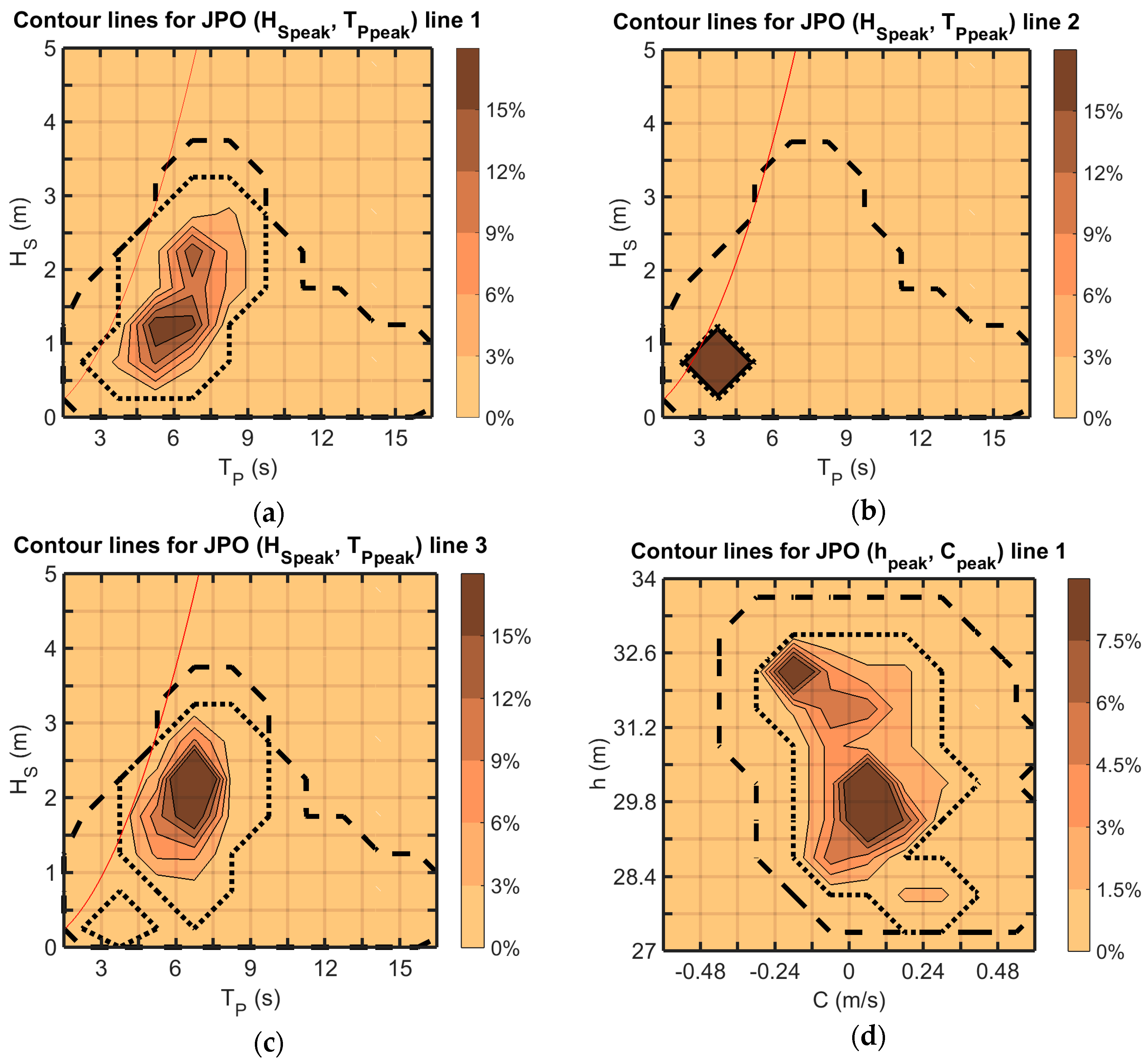
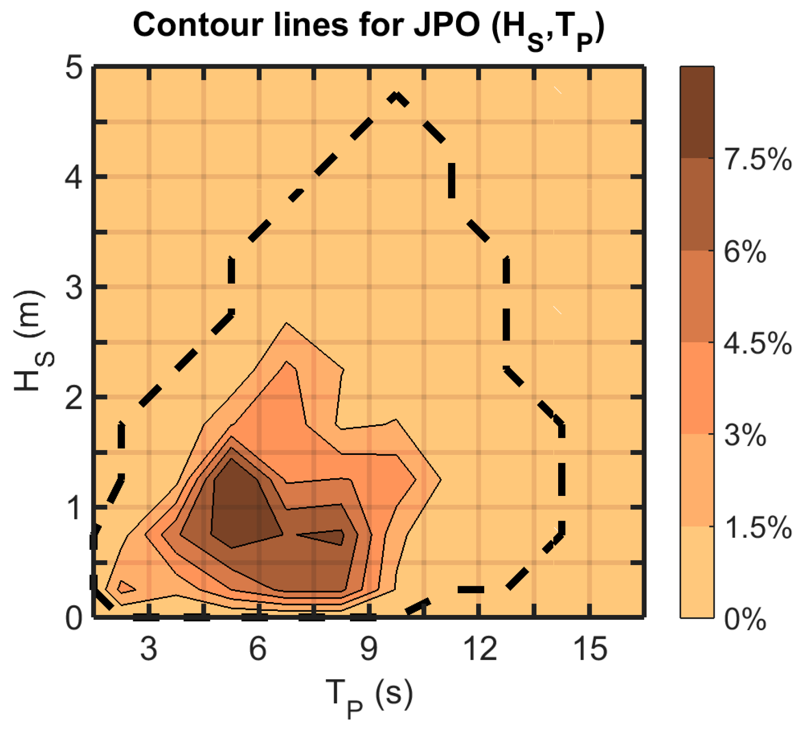
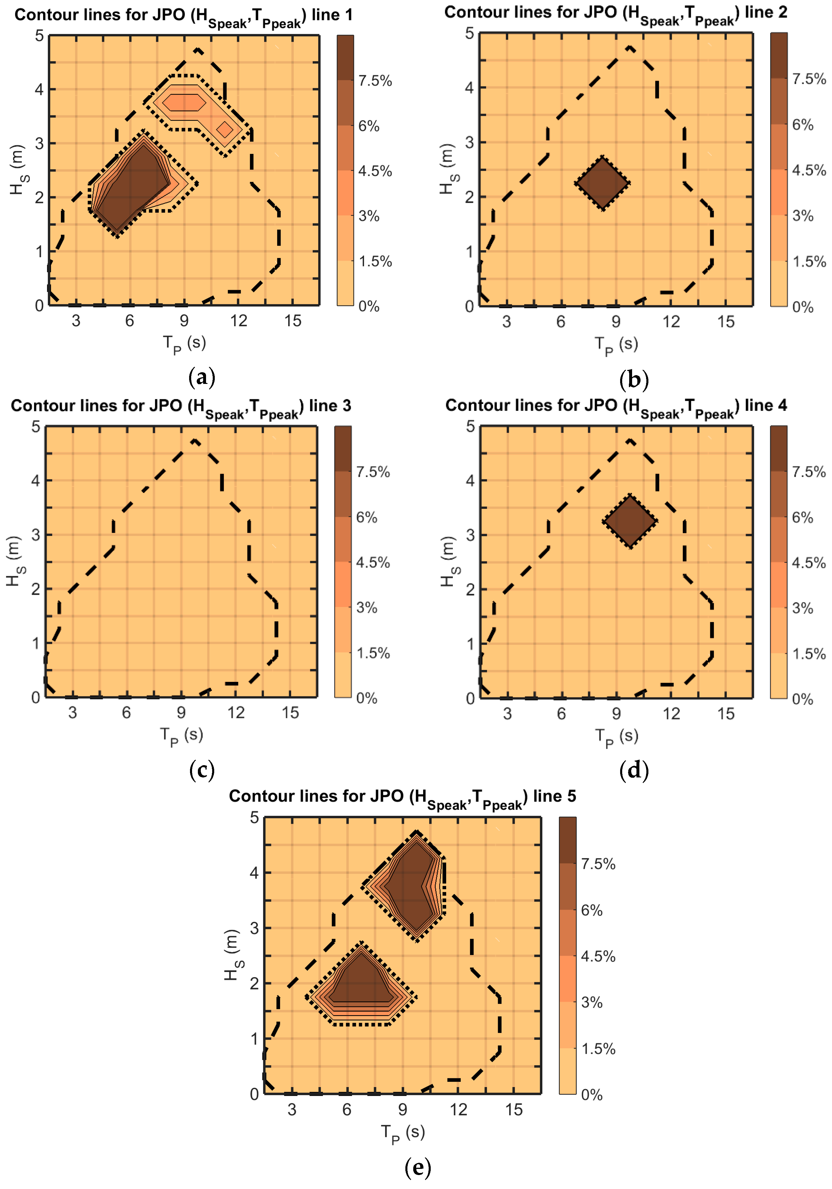
The results have separately described the general environmental conditions measured at the test sites and the environmental conditions that were associated with peak mooring loads.

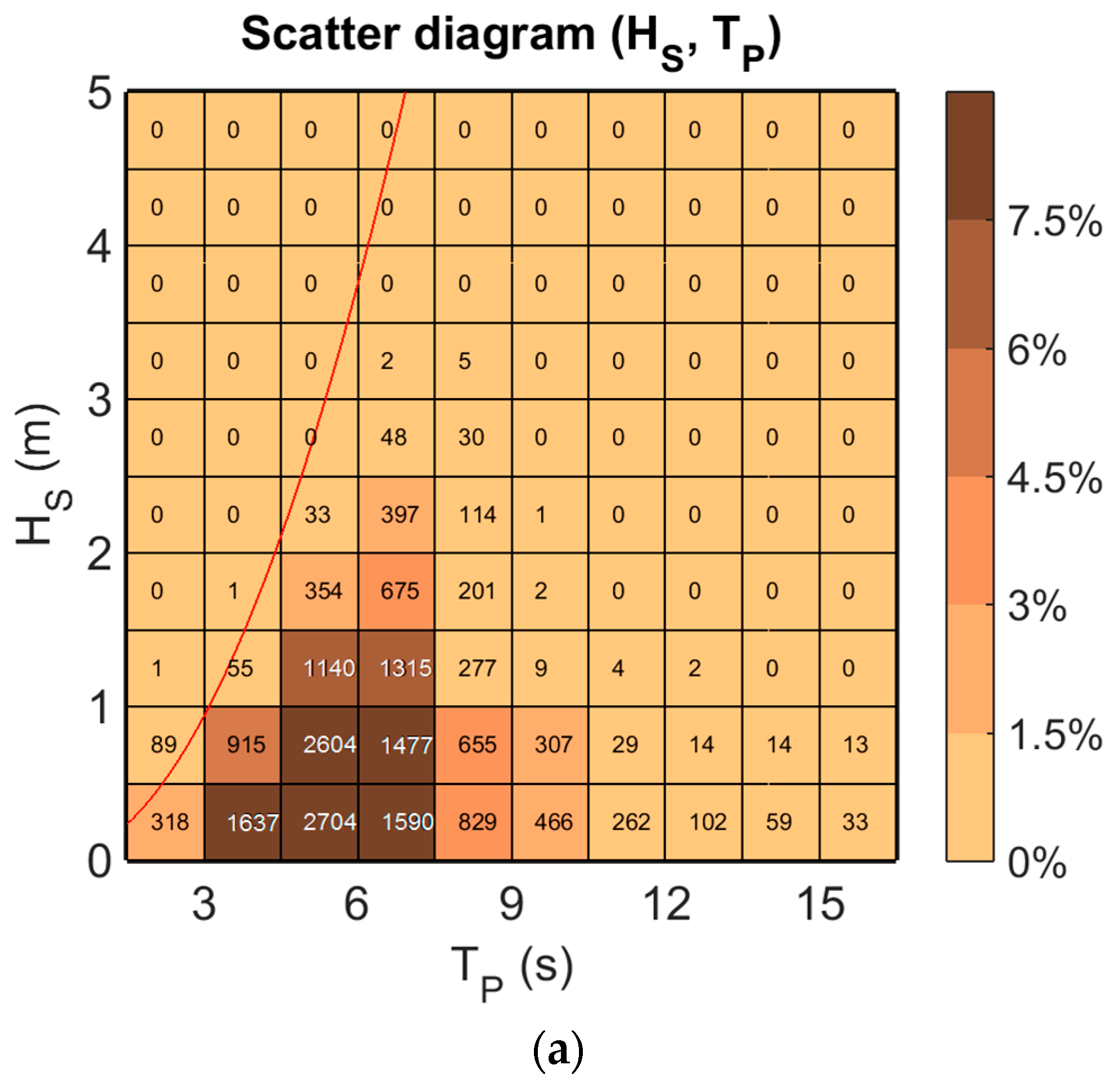
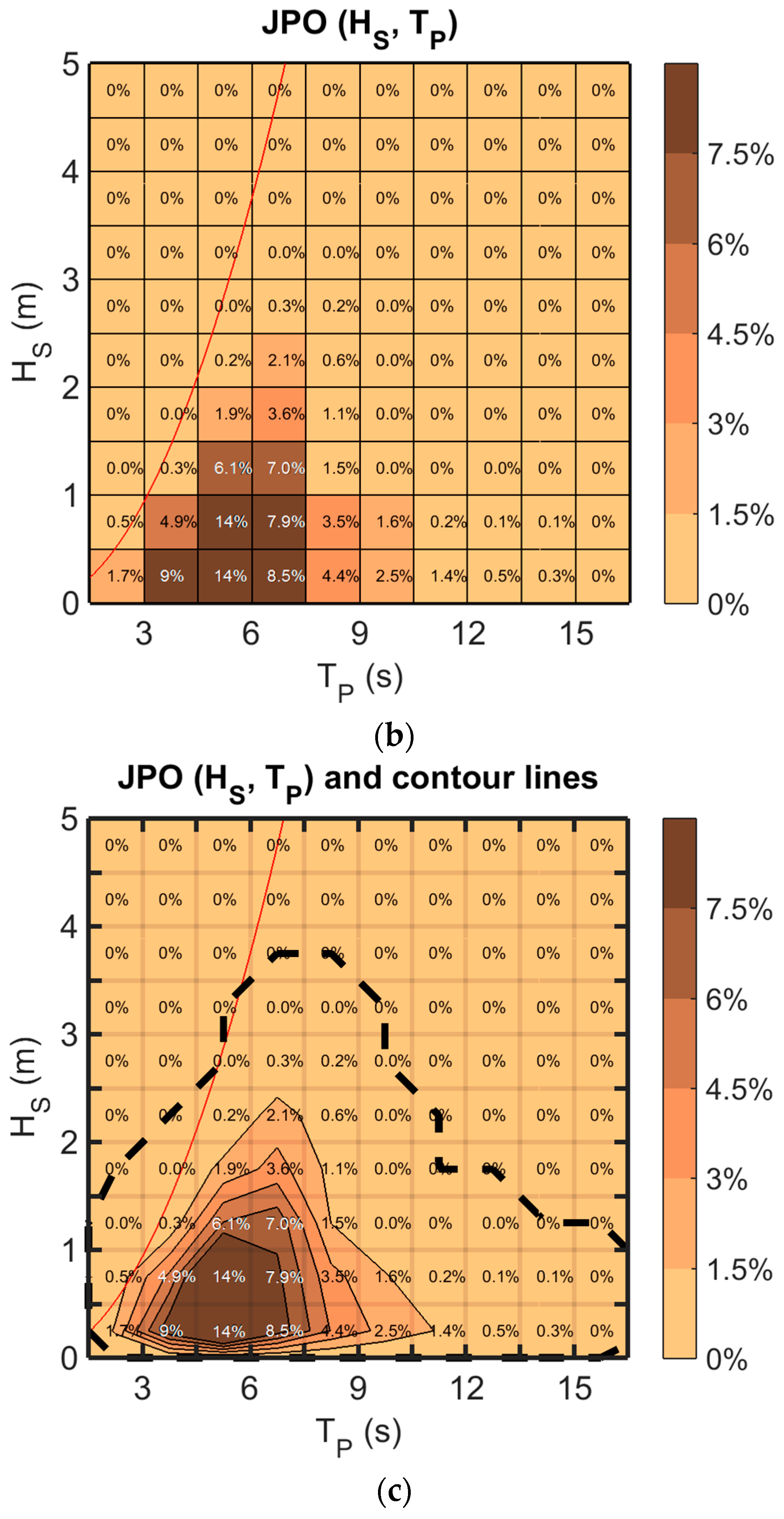
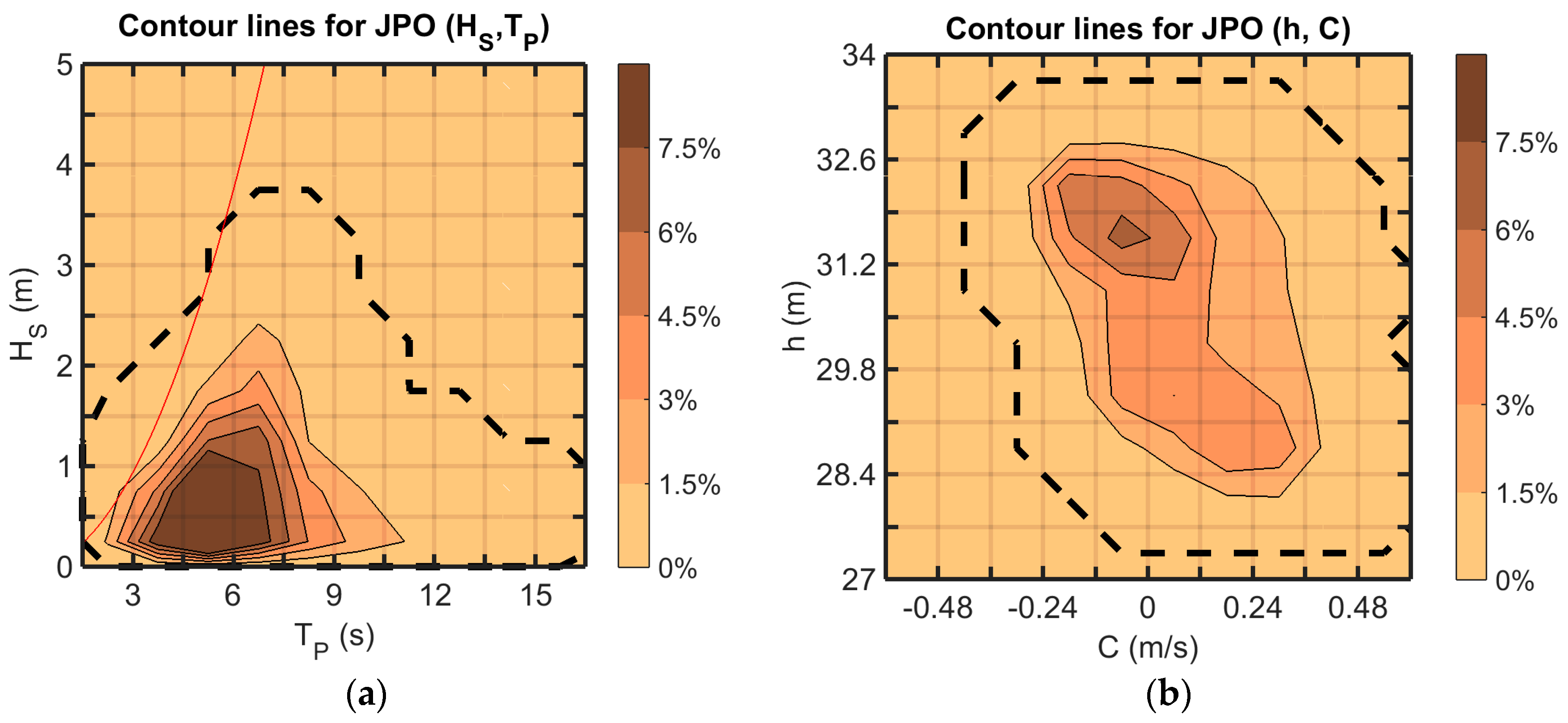
The joint percentage of occurrences of the wave conditions associated with peak mooring loads H_{S peak} and T_{P peak} is compared to the joint percentage of occurrences of the general wave conditions H_S and T_P. In addition, when available, the joint percentage of occurrences of the tidal conditions associated with peak mooring loads C_peak and h_peak is compared to the joint percentage of occurrences of the general tidal conditions C and h. These investigations give insight into specific and more general considerations. Specific considerations are the location of the measured peak mooring loads on the measured scatter diagram, the wave directions associated with peak mooring loads and the tidal conditions associated with peak mooring loads. More general considerations are the influence and meaning of the parameters chosen to isolate peak mooring loads, the improvement of MEC mooring design, the improvement of MEC mooring standards and the limitations of this study. These aspects are discussed in the following.

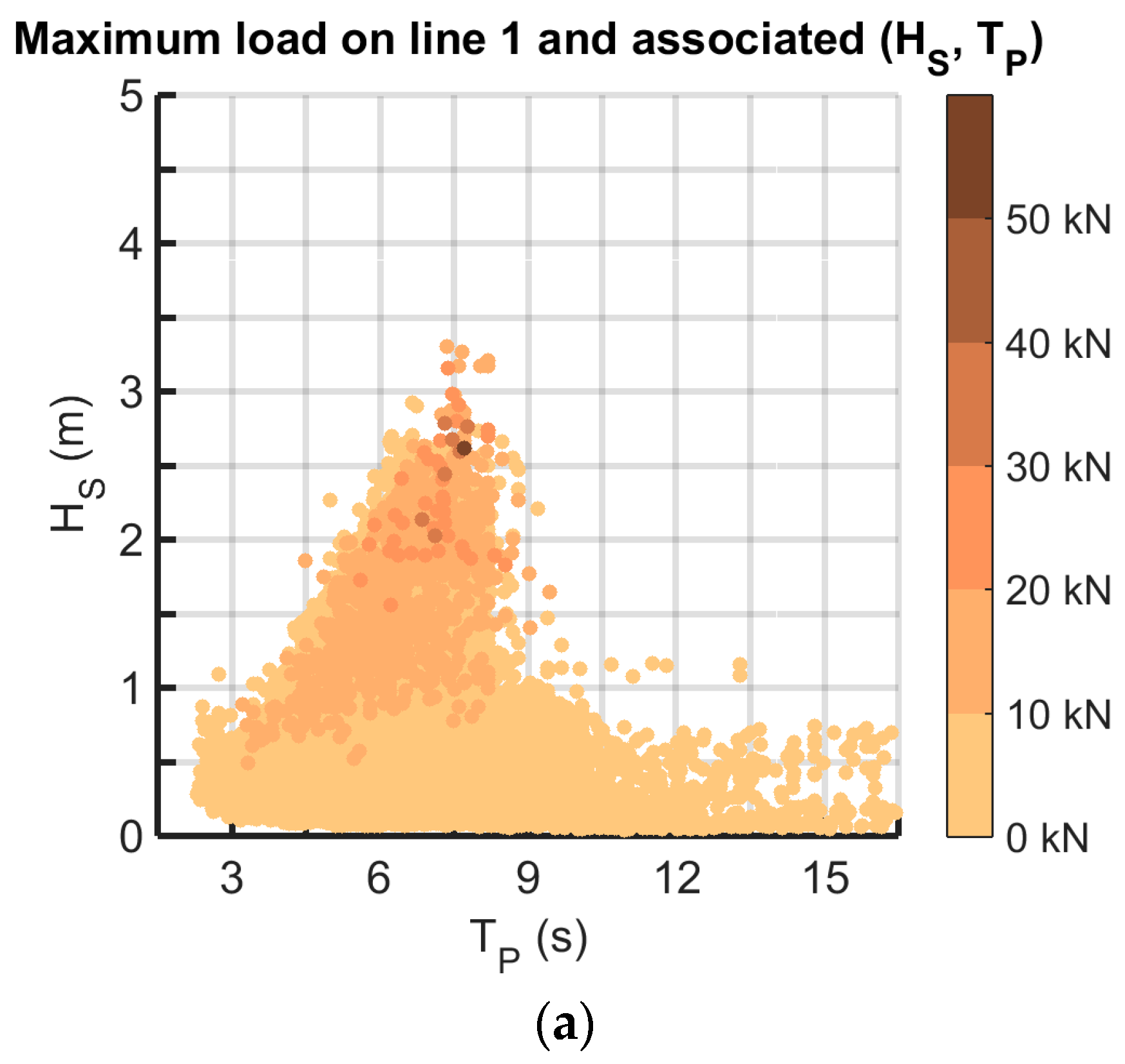
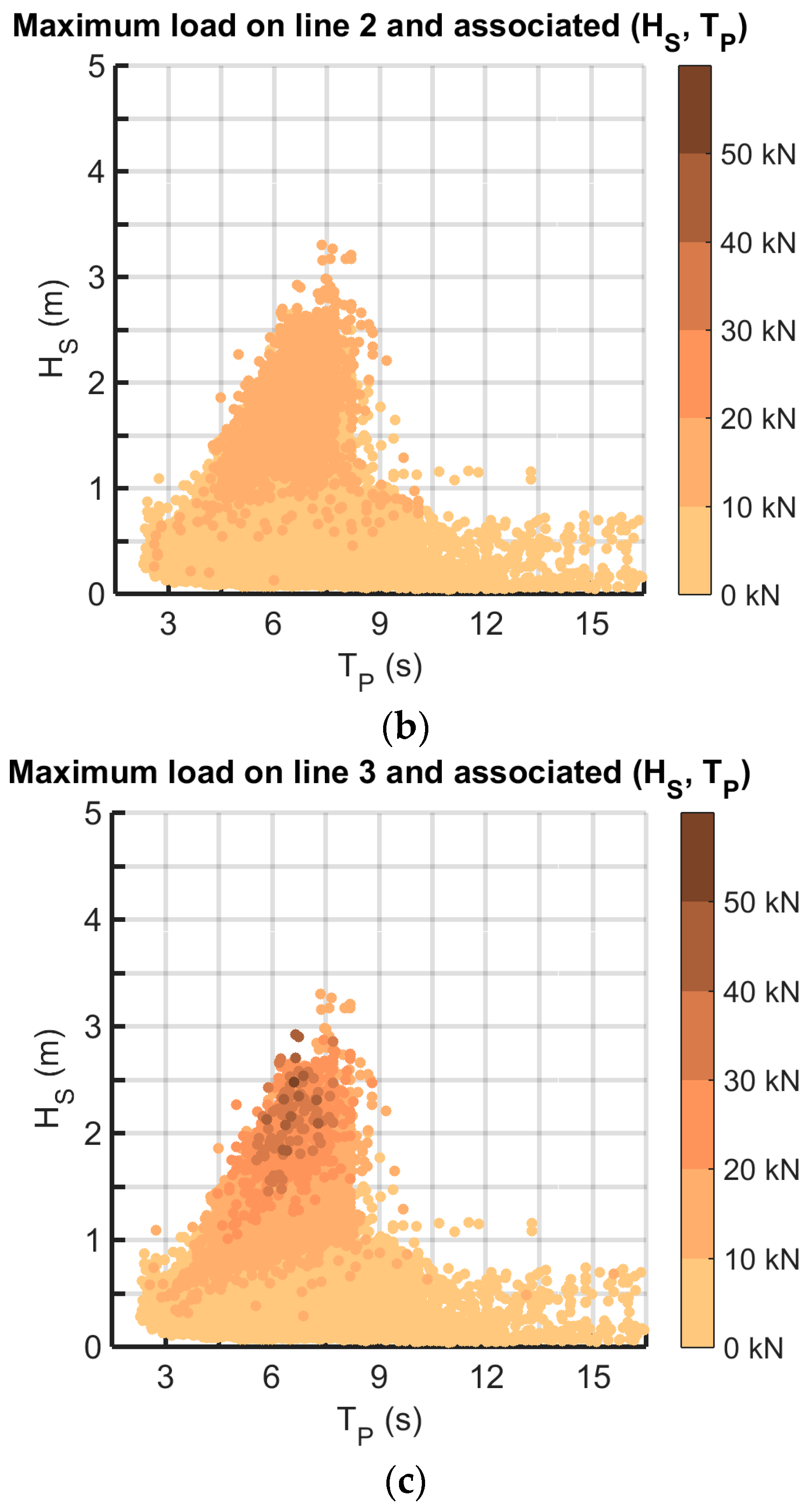
The results indicate that the peak mooring loads were more frequent inside the scatter diagram of the measured sea states (for moderate sea states) than on its external contour line. This can be clearly seen at both installations in Figure 11a–c (SWMTF) and Figure 13a–e (Bolt 2 Lifesaver).

Due to short-term response variability, the maximum mooring load for a given duration and for a given sea state is not a single value, but a random variable following the extreme value distribution (EVD), which is mainly dependent on H_S and on the mooring system design. The operational sea states were observed a large number of times, so higher mooring loads were more likely to occur for operational sea states representing a higher fractile of the EVD.

Ambühl [16] similarly noticed that large mooring loads on MEC moorings may occur during operation and not for extreme sea states when the device is in storm protection mode. The findings regarding the occurrence and potential severity of peak loads within this study and [16] emphasise that it is essential to undertake a detailed fatigue and peak load assessment, considering all operation sea states at an early design phase to avoid field failure.

Table 7. Natural period for the SWMTF moored structure.

	Natural Period
Surge/sway	24.8 s
Heave	2.0 s
Roll/pitch	2.4 s
yaw	6.3 s

indicated the natural period of the SWMTF moored system. The natural period is approximately 2 s for the heave and pitch motion. Figure 11a–c shows the joint percentage of occurrences of the wave conditions associated with peak mooring loads H_{S peak} and T_{P peak}. Peak mooring loads most frequently occurred for T_{P peak} around 6 s. This result indicates that the peak mooring loads are not directly driven by a resonant pitch or heave motion of the moored system. The measurements of the six DOF buoy motion, as well as the understanding of the wave elevation at the buoy can be used in the future to gain understanding of the mechanisms behind peak mooring loads.

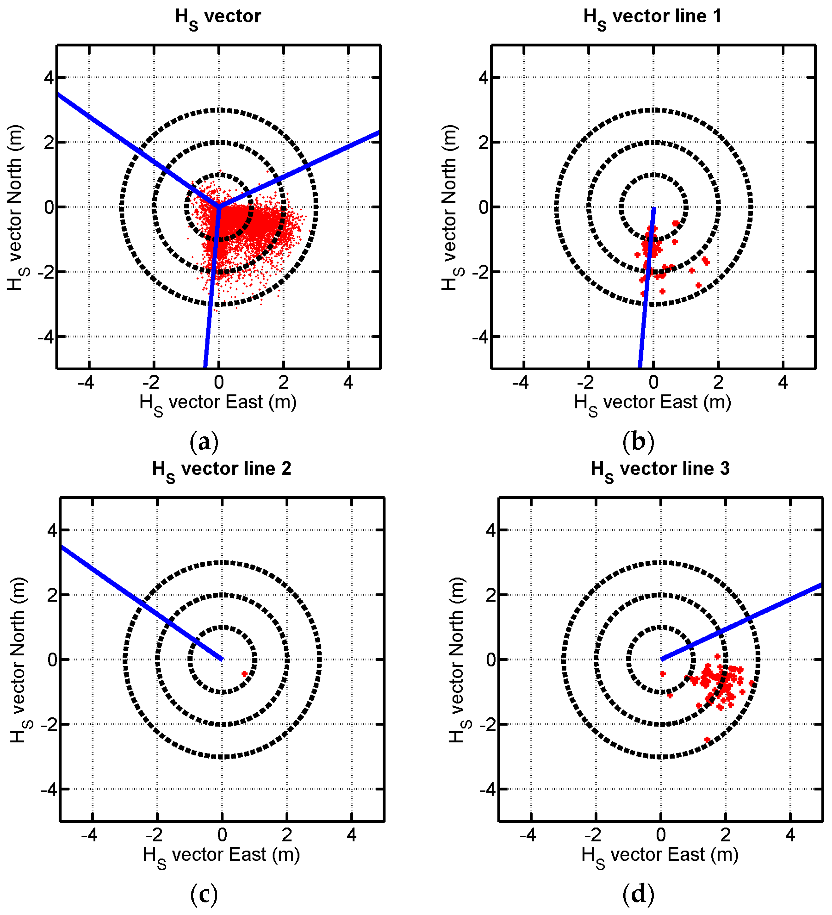
Results indicated that peak mooring loads occurred for a low value of H_S if the mooring line was aligned with the wave direction (Table 6). Figure 14a–d plots a vector H_{S vec} (red dots) with an amplitude equal to H_S and a direction equal to the peak direction D_P, associated with the peak period T_P. In Figure 14a, the three mooring lines are drawn (blue lines), while in Figure 14b–d, only one mooring line is drawn. Figure 14a plots H_{S vec} for the general environmental conditions, while Figure 14b–d plots H_{S vec} for the wave conditions associated with peak mooring loads on mooring lines 1–3, respectively. Figure 14a shows that two wave climates are occurring at SWMTF: one with waves coming from the east, the other with waves coming from the south. The mooring configuration of SWMTF was orientated to have the easterly sea states between mooring lines 1 and 3. The consequences of this choice can be observed in Figure 14b–d. Figure 14d indicates that no waves were able to align with line 3, resulting in peak mooring loads mainly for high H_S values. In Figure 14b, it can be observed that the waves coming from the south are able to align with line 1, resulting in peak mooring loads, even at low H_S, with wave heights below 1 m. These results indicate that directional contours could be introduced for the mooring design of any system installed in a location with different dominating wave directions in order to optimise the mooring configuration accordingly.

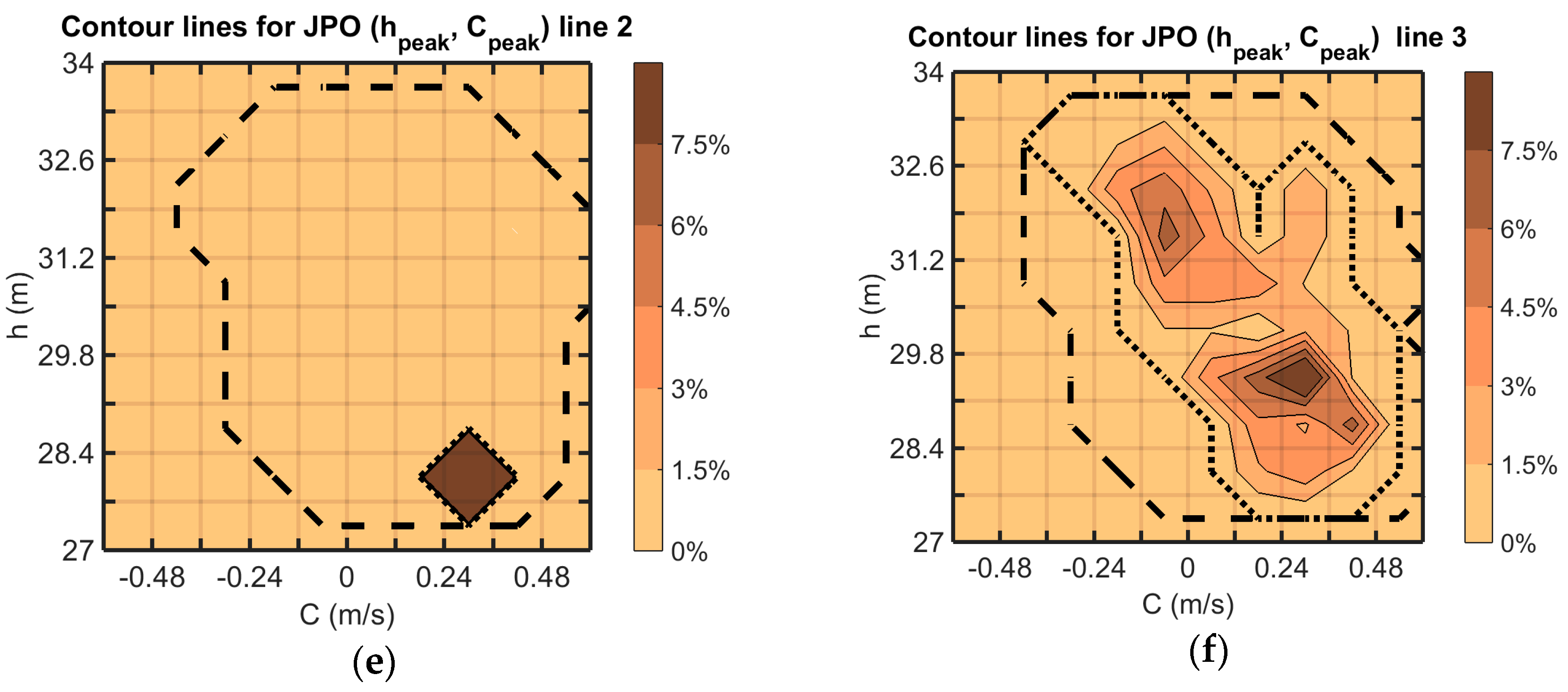
Tidal variations and the change in current direction also need to be taken into account for the mooring design. Based on the SWMTF results (Figure 11d–f), it can be observed that peak mooring loads are occurring both for low and high tides. The number of occurrences of peak mooring loads seems to be higher for low tidal conditions. However, the number of data points available is relatively low, and more data would be required in order to gain more confidence in this result. This result could be explained by the fact that the pre-tension in the mooring system is reduced for low tide, which consequently can lead to snatch loads [17]. The mooring system should be carefully designed for low tide conditions, but other tidal ranges have to be investigated during the design process because peak mooring loads also occur for high tide conditions. Standards, such as Det Norske Veritas DNV-OS-E301 [15] and American Petroleum Institute API RP 2SK [18], do not give specific recommendations for tidal variations, but they indicate that mooring design should be done for applicable water depths and currents. Based on the results of this study, several tidal elevations should be considered for MEC mooring design with an emphasis on low tide conditions.

The design of a mooring system can be complex if the tidal range is significant to the nominal water depth.

Table 8. Tidal variations compared to water depth at different wave energy sites.

Location		Scale	Nominal Water Depth	Tidal Range	Tidal Range/Nominal Water Depth
Nursery site
	SWMTF	1/3	27	5.4	20%
	FaBTest [16]	1	45 (15–55)	6	13%
	Galway Bay [19]	1/4	23	4	17%
Wave energy facility
	WaveHub [20]	1	55 (50–60)	7.3	13%
	EMEC Billia Croo	1	~50	6	12%

compares the nominal water depth and the tidal range at some nursery sites and wave energy facilities. It identifies that pre-tension variations caused at some sites, with a comparatively large tidal range to water depth ratio, could lead to design difficulties of the mooring system.

The tidal range needs to be accommodated by the mooring system, either by a specific mooring configuration or mooring materials. For example, the mooring tethers discussed by Thies et al. [17] can accommodate the tidal range. For the two mooring configurations presented in this paper, the tidal range was accommodated by chains lying on the seabed and lifted for high tide conditions. However, these chains add weight on the floating structure, which may be prejudicial to the power production.

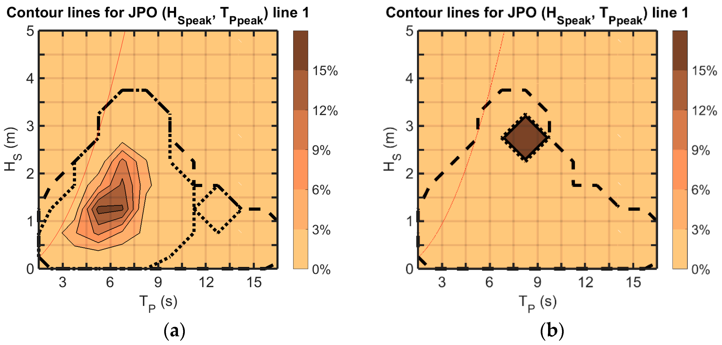
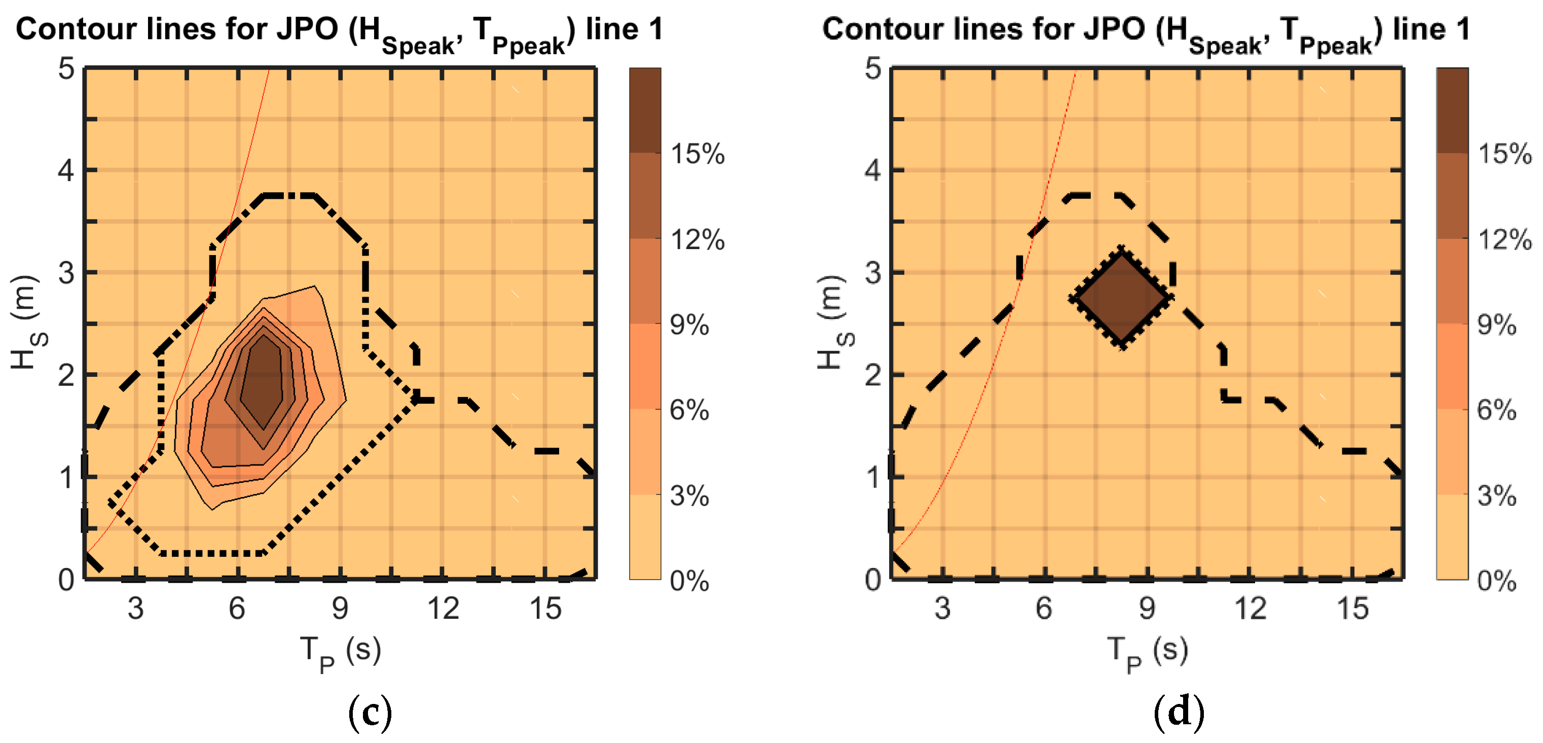
Table 6 gives a first indication of the influence of the parameters τ and K, which have been used in this paper to detect peak mooring loads. The percentage of sea states considered as containing peak mooring loads is indicated in this table for different τ and K combinations. It is of interest to gain more insight into the influence of τ and K on the detection of peak mooring loads. Whilst the analysis method is generic and applicable to different sites and devices, the individual parameters depend on the device characteristics, the site conditions and of course the mooring configuration and materials. As such, a sensitivity study is recommended to determine the specific parameters. The environmental conditions associated with peak mooring loads on mooring line 1 at SWMTF, shown in Figure 11a, have been plotted for different τ and K parameter values. The results of this sensitivity study are presented in Figure 15a–d. For lower values of τ, the JPO plots are similar, irrespective of K: peak loads still occur inside the scatter diagram, but they occur for sea states with higher H_S when τ increases and with lower H_S when τ decreases. For higher values of τ irrespective of K, only a few peak loads have been detected, and therefore, these results are difficult to use for general conclusions. Hence, the chosen values for τ and K must strike a balance of isolating peak loads (requiring high values) whilst capturing a sufficient amount of peak loads.

Some parameters could be further investigated to reduce the number of occurrences of peak mooring loads:

(a)

An increase of the pre-tension of the mooring system would reduce the number of occurrences of peak mooring loads, as suggested by the semi-taut configuration discussed by Johanning and Smith [21]. However, this should be balanced with the power production for a WEC device. A high pre-tension would reduce the motion of the floating structure and consequently will have an effect on the power production in the case of a motion-dependent wave energy device. With a semi-taut configuration, it would also be difficult to achieve a sufficiently high pre-tension for low tide, while achieving a reasonably low pre-tension for high tide.

(b)

An increase in the number of lines can also reduce the number of peak mooring loads. The results from the Bolt-2 Lifesaver mooring with five mooring lines cannot be directly compared to the SWMTF mooring with three mooring lines, as the period and duration of tests were different, and the floating structures are considerably different in size and mass. However, this solution is not cost effective because of the cost of the extra mooring lines, and it may also affect the power production by restraining the motion of the floating structure.

(c)

If the installation site has a limited number of wave directions and a low number of mooring lines, the mooring system can be oriented to avoid the worst wave climate. However, the seabed properties also have to be considered. The presented installations use drag embedment anchors, which require a soft soil, e.g., sand or clay.

The findings in this paper indicate that specific MEC design procedures would be beneficial. Currently, MEC devices are largely designed following offshore standards, with a tendency for too conservative design assumptions, leading to overdesigned mooring systems [22]. Design calculations could be conducted inside the scatter diagram, during operations. These calculations are most of the time already conducted for PTO optimisation and survival. MEC mooring systems could also be designed following a load and resistance factor design (LRFD) method [23], which is well suited to a given MEC mooring system.

One of the limitations of this study is that the two test sites used for this study are close to each other, with similar sheltered wave conditions and similar tidal conditions, and installed for a relatively short period of time. The two use similar multi-leg catenary moorings. The positive point is that some confidence can be gained in the results by observing similar results at both facilities and by comparing and explaining the differences. One of the main differences between both facilities is that FaBTest is in a more exposed location. This can be observed in the general wave condition results with more bins populated in the wave scatter diagram at FaBTest than at SWMTF, for a shorter sea trial time. Furthermore, the Bolt-2 Lifesaver device was operational, and the results did not consider if the PTOs were working or not. Further investigations could be conducted to assess if the mooring loads are reduced when the PTOs are active.

7. Conclusions

The outcomes of this study are some of the first published contributions based on extensive field load measurements of floating MEC systems. This paper has assessed the influence of environmental conditions on peak mooring loads. Some particular environmental conditions were more frequently associated with peak mooring loads.

The same methodology could be applied at different sites, for different MEC devices and alternative mooring configurations. This research will serve as a base for future studies aiming at understanding the individual hydrodynamic behaviour of floating structures and their mooring systems, leading to peak mooring loads. The objective is to find design solutions to mitigate peak mooring loads whilst avoiding the costly overdesign of mooring systems or compromising with the power production. The procedure and methodology presented in this paper will assist device developers, certification agencies and engineering companies involved in the development of dynamic MEC mooring systems to evaluate, refine and mitigate peak mooring load conditions.

References

1. Clément, A.; McCullen, P.; Falcao, A.; Fiorentino, A.; Gardner, F.; Hammarlund, K.; Lemonis, G.; Lewis, T.; Nielsen, K.; Petroncini, S.; et al. Wave energy in Europe: Current status and perspectives. Renew. Sustain. Energy Rev. 2002, 6, 405–431. [Google Scholar] [CrossRef]
2. Fitzgerald, J. Position Mooring of Wave Energy Converters. Ph.D. Thesis, Chalmers University of Technology, Göteborg, Sweden, 2009. [Google Scholar]
3. Harris, R.E.; Johanning, L.; Wolfram, J. Mooring systems for wave energy converters: A review of design issues and choices. In Proceedings of the 3rd International Conference on Marine Renewable Energy (MAREC), Blyth, UK, 7–9 July 2004.
4. Harnois, V.; Parish, D.; Johanning, L. Physical measurement of a slow drag of a drag embedment anchor during sea trials. In Proceedings of the International Conference on Ocean Energy (ICOE), Dublin, Ireland, 17–19 October 2012.
5. Johanning, L.; Spargo, A.W.; Parish, D. Large scale mooring test facility—A technical note. In Proceedings of the 2nd International Conference on Ocean Energy (ICOE), Brest, France, 15–17 October 2008.
6. Thies, P.R.; Johanning, L.; Harnois, V.; Smith, H.C.M.; Parish, D.N. Mooring line fatigue damage evaluation for floating marine energy converters: Field measurements and prediction. Renew. Energy 2013, 63, 133–144. [Google Scholar] [CrossRef]
7. Harnois, V.; Weller, S.D.; Johanning, L.; Thies, P.R.; Le Boulluec, M.; Le Roux, D.; Soulé, V.; Ohana, J. Numerical model validation for mooring systems: Method and application for wave energy converters. Renew. Energy 2015, 75, 869–887. [Google Scholar] [CrossRef] [Green Version]
8. Teledyne RD Instruments. WavesMon v3.08 User’s Guide. 2011. Available online: http://new.comm-tec.com/Docs/Manuali/RDI/WavesMon%20Users%20Guide.pdf (accessed on 1 April 2016).
9. Hjetland, E.; Bjerke, I.; Tjensvoll, G.; Sjolte, J. A brief introduction to the bolt-2-wave project. In Proceedings of the 9th European Wave and Tidal Energy Conference (EWTEC), Southampton, UK, 5–9 September 2011.
10. FaBTest. Description of Site Characteristics and Eligible Test Installations. 2012. Available online: http://fabtest.com/sites/default/files/Appendix-9-FaB-Test-site-characteristics-05.03.2012.pdf (accessed on 1 April 2016).
11. Fugro. SEAWATCH Mini II Buoy. 2010. Available online: http://www.oceanor.no/related/Datasheets-pdf/SW20_SEAWATCH_Mini_II_Buoy_FINAL.pdf (accessed on 1 April 2016).
12. Sanmuganathan, V. Seawatch Mini II Buoy; User Manual; Fugro GEOS Ltd.: Wallingford, UK, 2009. [Google Scholar]
13. EquiMar (Equitable Testing and Evaluation of Marine Energy Extraction Devices in terms of Performance, Cost and Environmental Impact). EquiMar Deliverable D2.2: Wave and Tidal Resource Characterisation. 2011. Available online: http://www.equimar.org/equimar-project-deliverables.html (accessed on 1 April 2016).
14. RD Instruments. Acoustic Doppler Current Profiler. Principles of Operations. A Practical Primer. 1996. Available online: http://misclab.umeoce.maine.edu/boss/classes/SMS_598_2012/RDI_Broadband%20Primer_ADCP.pdf (accessed on 1 April 2016).
15. DNV (Det Norske Veritas). DNV-OS-E301: Position Mooring; DNV: Oslo, Norway, 2013. [Google Scholar]
16. Ambühl, S.; Sterndorff, M.; Sørensen, J.D. Extrapolation of extreme response for different mooring line systems of floating wave energy converters. Int. J. Mar. Energy 2014, 7, 1–19. [Google Scholar] [CrossRef]
17. Thies, P.R.; Johanning, L.; McEvoy, P. A novel mooring tether for peak load mitigation: Initial performance and service simulation testing. Int. J. Mar. Energy 2014, 7, 43–56. [Google Scholar] [CrossRef] [Green Version]
18. API (American Petroleum Institute). API RP 2SK: Recommended Practice for Design and Analysis of Stationkeeping Systems for Floating Structures; API: Washington, DC, USA, 2005. [Google Scholar]
19. MARINET. SEAI_OEDU - National Wave Energy Test Site, Galway Bay. Available online: http://www.fp7-marinet.eu/SEAI_OEDU-wave-energy-test-site-galway-bay.html (accessed on 1 April 2016).
20. JP KENNY. SW Wave Hub—Metocean design basis. 2009. Available online: http://www.wavehub.co.uk/downloads/Resource_Info/Metocean_design_basis_Metoc_JP_Kenny_Report_2009.pdf (accessed on 1 April 2016).
21. Johanning, L.; Smith, G.H.; Wolfram, J. Measurements of static and dynamic mooring line damping and their importance for floating WEC devices. Ocean Eng. 2007, 34, 1918–1934. [Google Scholar] [CrossRef]
22. Paredes, G.M.; Bergdahl, L.; Palm, J.; Eskilsson, C.; Pinto, F.T. Station keeping design for floating wave energy devices compared to floating offshore oil and gas platforms. In Proceedings of the 10th European Wave and Tidal Energy Conference (EWTEC), Aalborg, Denmark, 2–5 September 2013.
23. DNV (Det Norske Veritas). Classification Notes 30.6: Structural Reliability Analysis of Marine Structures; DNV: Oslo, Norway, 1992. [Google Scholar]
Figure 1. South West Mooring Test Facility (SWMTF) and the Falmouth Bay Test Site (FaBTest) locations, adapted from the United Kingdom Hydrographic Office (UKHO) admiralty chart. ADCP: acoustic Doppler current profiler.
Jmse 04 00029 g001
Figure 2. SWMTF arrangement and instrumentation: (a) buoy; (b) tri-axial (left) and axial (right) mooring load cells and back-up rope (white); (c) plan view layout of the mooring system and ADCP (wave and current sensor) and (d) ADCP in its frame being installed.
Jmse 04 00029 g002
Figure 3. Bolt-2 Lifesaver arrangement and instrumentation: (a) floating structure; (b) mooring load cell; (c) plan view layout of the mooring system and wave buoy; and (d) adjacent wave buoy.
Jmse 04 00029 g003
Figure 4. Example of a 10-min record of mooring load on line 1 at SWMTF showing the value during a storm (17 November 2010) and a comparison of the values with a load factor K and a minimum threshold τ.
Jmse 04 00029 g004
Figure 5. Example of sea trial measurements for several days (red dots) and the detection of peak mooring loads and their corresponding environmental conditions (blue circles): at SWMTF: (a) HS; (b) TP; (c) C; (d) h; (e) maximum mooring load on line 1; and (f) standard score of the maximum mooring load Smax on line 1; at the Bolt-2 Lifesaver installation: (g) HS; (h) TP; (i) maximum mooring load on line 1; and (j) standard score of the maximum mooring load Smax on line 1.
Jmse 04 00029 g005
Figure 6. Example of current magnitude data recorded by the ADCP at SWMTF through the water column for several days.
Jmse 04 00029 g006
Figure 7. Examples based on the SWMFT wave data used in this paper of: (a) the scatter diagram, showing the number of occurrences of sea states for a given range of wave parameters HS and TP; (b) the joint percentage of occurrences (JPO) of sea states for a given range of wave parameters HS and TP; (c) the contour plot of JPO for wave data HS and TP. The red line corresponds to the breaking limit.
Jmse 04 00029 g007aJmse 04 00029 g007b
Figure 8. JPO for SWMTF general (a) wave measurements (HS, TP) and (b) current measurements (h, C).
Jmse 04 00029 g008
Figure 9. Summary of the measured maximum mooring loads at SWTMF and of the associated environmental conditions for (ac) lines 1–3.
Jmse 04 00029 g009aJmse 04 00029 g009b
Figure 10. Summary of the measured standard score of the maximum mooring loads Smax at SWTMF and of the associated environmental conditions for (ac) lines 1–3.
Jmse 04 00029 g010aJmse 04 00029 g010b
Figure 11. JPO for SWMTF environmental conditions associated with peak mooring loads: JPO(HS peak, TP peak) on mooring lines (a) 1, (b) 2 and (c) 3; JPO(hpeak, Cpeak) on mooring lines (d) 1, (e) 2 and (f) 3. The large black dashed line is the external contour line of the general environmental conditions. The thin black dotted line is the external contour line of the environmental conditions associated with peak mooring load.
Jmse 04 00029 g011aJmse 04 00029 g011b
Figure 12. JPO(HS, TP) for the Bolt-2 Lifesaver general wave measurements.
Jmse 04 00029 g012
Figure 13. JPO for the Bolt-2 Lifesaver wave conditions associated with peak mooring loads: JPO(HS peak, TP peak) on mooring lines (a) 1, (b) 2, (c) 3, (d) 4 and (e) 5. The large black dashed line is the external contour line of the general environmental conditions. The thin black dotted line is the external contour line of the environmental conditions associated with peak mooring load.
Jmse 04 00029 g013
Figure 14. HS vector summarising the amplitude of HS during a sea state and the associated peak wave direction DP (here, the wave direction is the incoming direction) (a) for the general wave conditions and for the sea states associated with peak mooring loads on mooring lines (b) 1, (c) 2 and (d) 3.
Jmse 04 00029 g014
Figure 15. JPO for SWMTF environmental conditions associated with peak mooring loads: JPO(HS peak, TP peak) on mooring line 1, (a) with K = 5 and τ = 7.5 kN, (b) with K = 10 and τ = 7.5 kN, (c) with K = 5 and τ = 12.5 kN and (d) with K = 10 and τ = 12.5 kN. The large black dashed line is the external contour line of the general environmental conditions. The thin black dotted line is the external contour line of the environmental conditions associated with peak mooring load.
Jmse 04 00029 g015aJmse 04 00029 g015b