Performance Assessment of NAMI DANCE in Tsunami Evolution and Currents Using a Benchmark Problem

Abstract

Numerical modeling of tsunami evolution, propagation, and inundation is complicated due to numerous parameters involved in the phenomenon. It is important to assess the performance of numerical codes that solve tsunami motion, as well as flow and velocity patterns. NAMI DANCE is a computational tool developed for the modeling of long waves. It provides numerical modeling and efficient visualization of tsunami generation, propagation, and inundation mechanisms and computes the tsunami parameters. In the theory of long waves, the vertical motion of water particles has no effect on the pressure distribution. Based upon this approximation and neglecting vertical acceleration, the equations of mass conservation and momentum are reduced to two-dimensional depth-averaged equations. NAMI DANCE uses finite difference computational method to solve linear and nonlinear forms of depth-averaged shallow water equations in long wave problems. In this study, NAMI DANCE is applied to a benchmark problem which was discussed in the 2015 National Tsunami Hazard Mitigation Program (NTHMP) annual meeting in Portland, USA. The benchmark problem features a series of experiments in which a single solitary wave propagates up a triangular shaped shelf which has an offshore island feature. The problem provides detailed free surface elevation and velocity time series in the vicinity of the island. The comparison of the results showed that NAMI DANCE is able to satisfactorily predict long wave evolution, propagation, amplification, and tsunami currents.

1. Introduction

Tsunamis are large waves that are generated by the abrupt movement of the ocean floor caused by undersea earthquakes, underwater landslides, volcanic eruptions, or large meteorite strikes. Tsunami waves are accepted as the most destructive parameter of this phenomenon; however, currents that are triggered by large wave movements may be very fatal in some cases. Basin resonance and geometric amplification are two reasonably well-understood mechanisms for local magnification of tsunami impact in closed basins, and are generally the mechanisms investigated when estimating the tsunami hazard potential in a port or harbor; on the other hand, the understanding of and predictive ability for currents is lacking [1]. This study aims to investigate the sufficiency of two-dimensional depth-averaged shallow water equations in the estimation of tsunami evolution, propagation, and amplification as well as tsunami currents by using a numerical tool; namely NAMI DANCE. Since the 1970s, solitary waves have commonly been used to model tsunamis, especially in experimental and mathematical studies [2]. In this respect, the numerical code is applied to a benchmark problem which focuses on the evolution and propagation of a single solitary wave over complex bathymetry. The problem describes a series of experiments that analyze the transformation of a single solitary wave as it propagates up a triangular shaped shelf with an island feature located at the offshore point of the shelf. The currents that are formed in the vicinity of the island are also investigated in the experiments. The benchmark problem used in this study is Benchmark Problem #5 of the 2015 National Tsunami Hazard Mitigation Program (NTHMP) workshop which was held in Portland, USA [3]. By comparing the benchmark data and the numerical results, it is observed that two-dimensional depth-averaged shallow water equations give satisfactory results regarding tsunami wave evolution and currents and thus are sufficient tools to use while determining tsunami mitigation strategies.

2. Materials and Methods

2.1. The Numerical Model: NAMI DANCE

Tsunami numerical modeling by NAMI DANCE is based on the solution of a nonlinear form of long wave equations with respect to related initial and boundary conditions [4]. In general, the explicit numerical solution of nonlinear shallow water (NSW) equations is preferred since it consumes reasonable computer time and memory, and also provides the results in acceptable error limits [4]. NAMI DANCE is a numerical model which is able to simulate tsunami evolution, propagation and inundation. It has been developed by the collaboration of Ocean Engineering Research Center, Middle East Technical University, Turkey, and Special Research Bureau for Automation of Marine Researches, Russia [5,6]. NAMI DANCE uses C++ programming language and solves NSW equations using a staggered leapfrog numerical solution procedure. In the theory of long waves, the vertical motion of water particles is not considered since it has a negligible effect on the pressure distribution. Based upon this approximation, using necessary dynamic and kinematic conditions and including the bottom friction terms, the fundamental equations of NAMI DANCE, which are given Equations (1)–(5), are obtained and these equations are discretized by following the staggered leapfrog scheme.

$$\frac{\partial \eta }{\partial t}+\frac{\partial M}{\partial x}+\frac{\partial N}{\partial y}=0$$

(1)

$$\frac{\partial M}{\partial t}+\frac{\partial }{\partial x}\left(\frac{M^2}{D}\right)+\frac{\partial }{\partial y}\left(\frac{MN}{D}\right)+gD\frac{\partial \eta }{\partial x}+\frac{g{n}^2}{D^{\raisebox{1ex}{$7$}\!\left/ \!\raisebox{-1ex}{$3$}\right.}}M\sqrt{M^2+N^2}=0$$

(2)

$$\frac{\partial N}{\partial t}+\frac{\partial }{\partial x}\left(\frac{MN}{D}\right)+\frac{\partial }{\partial y}\left(\frac{N^2}{D}\right)+gD\frac{\partial \eta }{\partial y}+\frac{g{n}^2}{D^{\raisebox{1ex}{$7$}\!\left/ \!\raisebox{-1ex}{$3$}\right.}}N\sqrt{M^2+N^2}=0$$

(3)

$$M=u\left(h+\eta \right)=uD$$

(4)

$$N=v\left(h+\eta \right)=vD$$

(5)

where x and y are the horizontal axes; t is time; h is undisturbed flow depth; η is the vertical displacement above the undisturbed water surface; M and N are the discharge fluxes in x and y directions; u and v are particle velocities in x and y directions, respectively; n is the Manning’s roughness coefficient; g is the gravitational acceleration, and D is the total water depth given by h + η [6].

NAMI DANCE is able to compute (i) tsunami source from either rupture characteristics or predetermined wave form; (ii) propagation; (iii) arrival time; (iv) coastal amplification; (v) inundation (according to accuracy and grid size); (vi) distribution of current velocities and their directions at selected time intervals; (vii) relative damage levels according to drag and impact forces; (viii) time histories of water surface fluctuations; (ix) 3D plots of sea state at selected time intervals from different camera and light positions; and (x) animations of tsunami propagation [7]. NAMI DANCE has been applied to analytical, experimental, and field benchmark problems [8,9] for validation and verification [10,11,12,13,14] and also applied to several tsunami events [7,15,16,17,18].

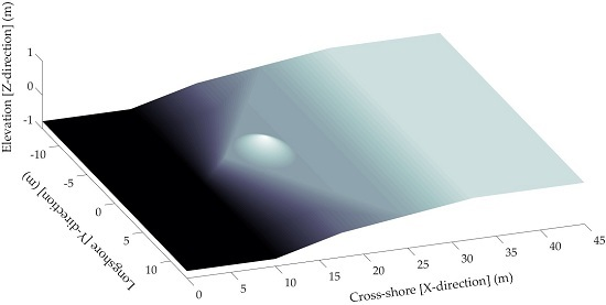
2.2. The Benchmark Problem

The benchmark problem describes a series of experiments which have a single solitary wave propagating up a triangular shaped shelf with an island feature located at the offshore point of the shelf. The series of experiments are conducted in a large wave basin which is 48.8 m long, 26.5 m wide and 2.1 m deep [19]. The basin is equipped with a piston-type wave maker powered by an electric motor and a wave board that consists of 29 independently functioning paddles, which is able to produce linear and nonlinear waves up to 0.8 m in height [19]. The walls and the underlying bathymetry of the basin are made of concrete in order to reduce the boundary effects due to friction [19]. The complex bathymetry is constructed symmetrically along the centerline of the basin. The water depth is kept constant at 0.78 m and hence the still water level (SWL) intersects the land at X = 25.75 m [19]. A single solitary wave with a height of 0.39 m is generated for each trial [19]. In the experiments, resistance and sonic wave gages are used to record the free surface elevation time series, and the velocity time series are recorded via acoustic Doppler velocimeters (ADVs) [19]. The bathymetry provided with the benchmark problem is given in Figure 1.

The free surface elevation time series are recorded at Y = 0.0 m at following X-locations: X = 7.5 m, 13.0 m, and 21.0 m; at Y = 5.0 m at following X-locations: X = 7.5 m, 13.0 m, and 21.0 m; and at X = 25.0 m at following Y-locations: Y = 0.0 m and 5.0 m. The velocity data are recorded at two locations: X = 13.0 m, Y = 0.0 m and z = 0.75 m and X = 21.0 m, Y = −5.0 m, and z = 0.77 m.

The input parameters that are necessary for numerical modeling are the XYZ dataset of the bathymetry and the free surface elevation time series of the incoming wave. The dimensions of these parameters are kept the same as the ones that are used in the experiments. Figure 2 shows the model bathymetry and the incoming wave, which is a single solitary wave with a height of 0.39 m. The free surface elevation time series of the incoming wave is inputted from the left border, i.e., X = 0.0 m along Y-axis. The model bathymetry is formed using structured grids. The spatial grid size, Δx, is selected as 0.05 m to achieve more accurate results. The time step, Δt, is selected as 0.001 s to ensure stability with 0.05 m grid size. The duration of each simulation is 20 s, which is sufficient to observe the maximum wave height and the effect of the island on the propagation of the solitary wave. It is observed that it takes approximately 1 h to complete each simulation using 12-Core CPUs.

3. Results

3.1. Free Surface Elevation Time Series

The free surface elevation is measured via wave gages which are placed offshore, near shore and in the vicinity of the island. The gages placed in the vicinity of the island make it possible to record and analyze the effect of the island on the propagation of the single solitary wave and wave currents. The comparison of the results regarding the free surface elevation time series is given in Figure 3.

The results revealed that depth-averaged NSW equations are able to satisfactorily predict the free surface elevation at gages 1, 4, 7, and 8. However, these equations fail to accurately estimate the free surface elevation in the vicinity of the island, i.e., at gages 2, 3, 5, and 6. It is known from the experimental observations that turbulence and relatively large wave currents are formed in the vicinity of the island; these are considered to play a role in the underestimation of maximum wave amplitudes.

3.2. Velocity Time Series

The velocity time series are measured via ADVs. The effect of the island on the direction and magnitude of wave currents is also recorded and analyzed. The comparison of the results regarding the wave currents is given in Figure 4.

The results showed that depth-averaged NSW equations are able to satisfactorily predict the velocity components in x-direction. On the other hand, the maximum velocity values in y-direction are underestimated even though the predicted and measured velocity components show a similar trend.

3.3. Performance Assessment of the Model

The credibility of a numerical model is directly related to its performance. Using numerical models, it is impossible to obtain the same outcomes as those in natural systems since natural systems are never closed and model results are not always unique. The expected outcome is an acceptable level of agreement between analytical/experimental/field data and model prediction, as well as sufficient accuracy of the model. The performance of numerical models can be assessed by demonstrating the agreement between observation and prediction. Models can only be evaluated in relative terms, and their predictive value is always debatable. There is a variety of different methods to assess the performance of numerical models. Error statistics is one of these tools.

Different types of errors are introduced to determine the correlation between the analytical/experimental/field data and model results. In National Oceanic and Atmospheric Administration (NOAA), two common errors are emphasized; namely, normalized root mean square error, NRMSE, and the error of the maximum value, MAX [20]. The percent NRMSE is applied within a space segment or time period to all observed data points. The main use of NRMSE is to assess the accuracy of a model in predicting the entire set of observed data; in other words, it is used to define the overall model performance. NRMSE deals with an error of absolute values and does not show the bias of the code’s prediction (i.e., underprediction or overprediction). MAX is used to quantify each model’s predictive accuracy for the maximum data point regardless of the location and time.

The formulas to evaluate percent NRMSE and MAX error values are given in Equations (6) and (7):

$$\text{NRMSE}=100\times \frac{1}{f{\left(x_i\right)}_{max}-f{\left(x_i\right)}_{min}}\sqrt{\frac{{\sum }^{\text{}}{\left(f\left(x_i\right)-y_i\right)}^2}{n}}$$

(6)

$$\text{MAX}=100\times \frac{\left|f{\left(x_i\right)}_{max}-y_{imax}\right|}{f{\left(x_i\right)}_{max}}$$

(7)

where f(x_i) represents the observed data and y_i represents the predicted data.

The benchmark problem discussed in this study features a series of experiments collecting free surface elevation and velocity data. The velocity computations in numerical models differ at shallow water depths because of the nature and limit of two-dimensional depth-averaged shallow water equations. Therefore, larger error limits are accepted for velocity comparisons in shallow water depths. The NRMSE and MAX error limits for velocity values for experimental benchmarks can be selected as 15% and 25%, respectively [20]. For free surface elevation time series, NRMSE and MAX error limits may be reduced to 15% and 10%, respectively [20]. Statistical error analysis is applied to the results given in Section 3.1 and Section 3.2. The results are listed separately for the free surface elevation time series, and velocity time series and are given in

Table 1. Error statistics of numerical results for free surface elevation time series recorded at each gage.

Free Surface Elevation (FSE)	% NRMSE	% MAX
Gage 1	0.60	0.02
Gage 2	7.30	19.30
Gage 3	15.00	17.60
Gage 4	2.60	2.60
Gage 5	7.20	18.80
Gage 6	8.70	8.20
Gage 7	4.50	7.30
Gage 8	5.00	6.80

and

Table 2. Error statistics of numerical results for horizontal velocity time series recorded at each gage.

Horizontal Velocity	% NRMSE	% MAX
Gage 2, U	8.25	18.90
Gage 2, V	16.00	27.90
Gage 9, U	10.75	15.00
Gage 9, V	16.00	28.60

.

4. Discussion

Nonlinear depth-averaged shallow water equations are commonly used to simulate the evolution and propagation of long waves offshore, near shore, and on the ground. These equations are solved using an explicit numerical scheme in which the staggered grid method in space and the leapfrog method in time are adopted. NAMI DANCE is one of many numerical tools that solve two-dimensional depth-averaged nonlinear shallow water equations to estimate the long wave behavior depending on bathymetry and topography. It is still controversial whether these equations predict tsunami currents accurately or not. In this study, the competence of depth-averaged NSW equations was tested using a benchmark problem. The results were analyzed in two aspects; free surface elevation and velocity time series. It is revealed that depth-averaged NSW equations satisfactorily predict the evolution, propagation, and amplification of long waves over complex bathymetry when turbulence effect is negligible. In the opposite case, the numerical results and observed data show a similar trend; however, the propagation and amplification of long waves are not accurately predicted. The turbulence and shoaling effects in the vicinity of the island, as well as the limitations of depth-averaged NSW equations, are considered to play a role in the underestimation of maximum wave amplitudes. The predicted and measured velocity components in x-direction are in good agreement with each other. The maxima of the velocity components in x-direction are reached. On the other hand, even though the predicted and measured velocity components in y-direction show a similar trend, the maximum velocity values are underestimated. Therefore, the prediction of the velocity components in y-direction needs improvement. Depth-averaged NSW equations may be a sufficient tool while developing tsunami mitigation strategies. However, long wave currents need further analysis in closed basins such as harbors and ports where they become a prominent parameter for the impact and drag on marine vessels, and also the resilience and endurance of coastal structures.

5. Conclusions

Numerical modeling of coastal hydrodynamics constantly gains importance in the world of coastal engineering due to the rapid development in computing technology. The modeling techniques have become more sophisticated and a large number of models can now be employed in a variety of coastal hydrodynamic problems. Accordingly, the performance assessment of numerical codes becomes crucial. The credibility of a numerical model has a direct relationship with its performance, which can be evaluated by indicating the level of agreement between observation and prediction. NAMI DANCE is one of many coastal models that solve two-dimensional depth-averaged NSW equations. This study investigated the performance of these equations in the estimation of long wave evolution, propagation, amplification, and long wave currents using NAMI DANCE. In this respect, the numerical code was applied to a benchmark problem which describes a series of experiments that analyze the transformation of a single solitary wave as it propagates up a triangular shaped shelf with an island feature located at the offshore point of the shelf. The results of this study indicate that depth-averaged NSW equations satisfactorily predict the evolution, propagation, and amplification of long waves over complex bathymetry when turbulence effect is negligible. On the other hand, NSW equations are not able to produce accurate results when the turbulence effects become dominant. Depth-averaged NSW equations may still be preferred while developing tsunami mitigation strategies. However, further studies on different benchmark problems are necessary to identify the performance and validity of depth-averaged NSW equations when the current behavior of long waves is investigated.

References

1. Lynett, P.J.; Borrero, J.C.; Weiss, R.; Son, S.; Greer, D.; Renteria, W. Observations and modeling of tsunami-induced currents in ports and harbors. EPSL 2012, 327, 68–74. [Google Scholar]
2. Madsen, P.A.; Fuhrman, D.R.; Schaffer, H.A. On the solitary wave paradigm for tsunamis. J. Geophys. Res. 2008, 113. [Google Scholar] [CrossRef]
3. NTHMP Mapping & Modeling Benchmarking Workshop: Tsunami Currents. Benchmark #5. Available online: http://coastal.usc.edu/currents_workshop/problems/prob5.html (accessed on 2 August 2016).
4. Onat, Y.; Yalciner, A.C. Initial stage of database development for tsunami warning system along Turkish coasts. Ocean Eng. 2013, 74, 141–154. [Google Scholar] [CrossRef]
5. Kian, R.; Yalciner, A.C.; Aytore, B.; Zaytsev, A. Wave Amplification and Resonance in Enclosed Basins; A Case Study in Haydarpasa Port of Istanbul. In Proceedings of the 2015 IEEE/OES Eleventh Current, Waves and Turbulence Measurement, St. Petersburg, VA, USA, 2–6 March 2015; Volume 11, pp. 1–7.
6. Patel, V.M.; Dholakia, M.B.; Singh, A.P. Emergency preparedness in the case of Makran tsunami: A case study on tsunami risk visualization for the western parts of Gujarat, India. Geomat. Nat. Hazards Risk 2016, 7, 826–842. [Google Scholar] [CrossRef]
7. Yalciner, A.C.; Pelinovsky, E.; Zaytsev, A.; Kurkin, A.; Ozer, C.; Karakus, H.; Ozyurt, G. Modeling and visualization of tsunamis: Mediterranean examples. In Tsunami and Nonlinear Waves, 1st ed.; Kundu, A., Ed.; Springer: Berlin, Germany, 2007; pp. 273–283. [Google Scholar]
8. Synolakis, C.E.; Bernard, E.N.; Titov, V.; Kanoglu, U.; Gonzalez, F. Validation and verification of tsunami numerical models. PAGEOPH 2008, 165, 2197–2228. [Google Scholar] [CrossRef]
9. Yalciner, A.C.; Zaytsev, A.; Kanoglu, U.; Velioglu, D.; Dogan, G.G.; Kian, R.; Sharghivand, N.; Aytore, B. NTHMP Mapping and Modeling Benchmarking Workshop: Tsunami Currents. Available online: http://coastal.usc.edu/currents_workshop/presentations/Yalciner.pdf (accessed on 2 August 2016).
10. Ozer, C.; Yalciner, A.C. Sensitivity study of hydrodynamic parameters during numerical simulations of tsunami inundation. PAGEOPH 2011, 168, 2083–2095. [Google Scholar]
11. Sozdinler, C.O.; Yalciner, A.C.; Zaytsev, A. Investigation of tsunami hydrodynamic parameters in inundation zones with different structural layouts. PAGEOPH 2014, 172, 931–952. [Google Scholar] [CrossRef]
12. Sozdinler, C.O.; Yalciner, A.C.; Zaytsev, A.; Suppasri, A.; Imamura, F. Investigation of hydrodynamic parameters and the effects of breakwaters during the 2011 Great East Japan Tsunami in Kamaishi Bay. PAGEOPH 2015, 172, 3473–3491. [Google Scholar] [CrossRef]
13. Velioglu, D.; Kian, R.; Yalciner, A.C.; Zaytsev, A. Validation and Performance Comparison of Numerical Codes for Tsunami Inundation. In Proceedings of the 2015 American Geophysical Union Fall Meeting, San Francisco, CA, USA, 14–18 December 2015.
14. Velioglu, D.; Kian, R.; Yalciner, A.C.; Zaytsev, A. Validation and Comparison of 2D and 3D Codes for Nearshore Motion of Long Waves Using Benchmark Problems. In Proceedings of the 2016 European Geosciences Union, Vienna, Austria, 17–22 April 2016.
15. Dilmen, D.I.; Kemec, S.; Yalciner, A.C.; Düzgün, S.; Zaytsev, A. Development of a tsunami inundation map in detecting tsunami risk in Gulf of Fethiye, Turkey. PAGEOPH 2015, 172. [Google Scholar] [CrossRef]
16. Heidarzadeh, M.; Krastel, S.; Yalciner, A.C. The state-of-the-art numerical tools for modeling landslide tsunamis: A short review. In Submarine Mass Movements and Their Consequences, 6th ed.; Sebastian, K., Jan-Hinrich, B., David, V., Michael, S., Christian, B., Roger, U., Jason, C., Katrin, H., Michael, S., Carl, B.H., Eds.; Springer: Bern, Switzerland, 2013; Volume 37, pp. 483–495. [Google Scholar]
17. Yalciner, A.C.; Gülkan, P.; Dilmen, D. I.; Aytore, B.; Ayca, A.; Insel, I.; Zaytsev, A. Evaluation of tsunami scenarios for western Peloponnese, Greece. Boll. Geofis. Teor. Appl. 2014, 55, 485–500. [Google Scholar]
18. Zahibo, N.; Pelinovsky, E.; Kurkin, A.; Kozelkov, A. Estimation of far-field tsunami potential for the Caribbean Coast based on numerical simulation. Sci. Tsunami Hazards 2003, 21, 202–222. [Google Scholar]
19. Swigler, D.T. Laboratory Study Investigating the Three-dimensıonal Turbulence and Kinematic Properties Associated with a Breaking Solitary Wave. Master’s Thesis, Texas A&M University, College Station, TX, USA, August 2009. [Google Scholar]
20. National Tsunami Hazard Mitigation Program. Proceedings and Results of the 2011 NTHMP Model Benchmarking Workshop. Available online: http://nws.weather.gov/nthmp/documents/nthmpWorkshopProcMerged.pdf (accessed on 21 July 2016).
Figure 1. The bathymetry provided with the benchmark problem.
Jmse 04 00049 g001
Figure 2. Model parameters: (a) bathymetry of the numerical model, NAMI DANCE; (b) incoming wave.
Jmse 04 00049 g002
Figure 3. Comparison of free surface elevation (FSE) results: (a) X = 7.5 m and Y = 0.0 m at Gage 1; (b) X = 13.0 m and Y = 0.0 m at Gage 2; (c) X = 21.0 m and Y = 0.0 m at Gage 3; (d) X = 7.5 m and Y = 5.0 m at Gage 4; (e) X = 13.0 m and Y = 5.0 m at Gage 5; (f) X = 21.0 m and Y = 5.0 m at Gage 6; (g) X = 25.0 m and Y = 0.0 m at Gage 7; (h) X = 25.0 m and Y = 5.0 m at Gage 8. Black line represents benchmark data, red line represents numerical results.
Jmse 04 00049 g003
Figure 4. Comparison of results: (a) horizontal velocity in x-direction, U, recorded at X = 13.0 m, Y = 0.0 m and Z = 0.75 m at Gage 2; (b) horizontal velocity in y-direction, V, recorded at X = 13.0 m, Y = 0.0 m and Z = 0.75 m at Gage 2; (c) horizontal velocity in x-direction, U, recorded at X = 21.0 m, Y = −5.0 m and Z = 0.77 m at Gage 9; (d) horizontal velocity in y-direction, V, recorded at X = 21.0 m, Y = −5.0 m and Z = 0.77 m at Gage 9. Black line represents benchmark data, red line represents numerical results.
Jmse 04 00049 g004