1. Introduction
Systematic analyses of large-scale Ocean Thermal Energy Conversion (OTEC) impacts and their possible feedback effects on the size of global OTEC resources have been few probably for two main reasons. On one hand, it is a dauntingly complex problem to tackle, even with the recent availability of massive computing capabilities; simplifying the modeling framework may prove expedient, but excessive simplifications also introduce limitations and are likely to cast doubts on any result. More importantly, the urgency of solving such a problem is bound to seem remote given the very slow pace of development afflicting OTEC technologies. From environmental and permitting perspectives, however, one should recognize an increasing tendency to expect a grasp of large-scale impacts for any given technology, even if a specific project is small and isolated.
The analysis of the impacts of large-scale OTEC development using a locally one-dimensional (1-D) framework was spearheaded by Martin and Roberts for the Gulf of Mexico [
1], when computing capabilities were very limited; the reduction of a fully three-dimensional problem was more easily justified in this case of a semi-enclosed body of water. Drawing on experience acquired with one-dimensional oceanic models applied to a newly proposed geo-engineering concept at global scales [
2,
3], the deep ocean sequestration of anthropogenic carbon dioxide, Nihous later probed the issue of large-scale OTEC resources with similar models [
4,
5,
6]. The limitations of this approach were never in doubt, since horizontal transport phenomena are dominant in the ocean, and the situation far more complex than represented in simple advection-diffusion models of the oceanic water column. In the absence of any rational method to assess global OTEC resources, though, the motivation for such studies was to be able to provide a starting point for future, more elaborate analyses, while identifying possible qualitative features of large-scale OTEC impacts, including self-limiting modifications of the vertical thermal structure of the ocean.
Studies of large-scale OTEC development using state-of-the-art three-dimensional (3-D) ocean general circulation models were initiated more recently [
7,
8,
9] and provided significant additional insight toward the evaluation of sustainable OTEC resources, and of the potential large-scale environmental effects associated with the widespread implementation of the OTEC technology. They were able, in particular, to predict geographically differentiated effects that a one-dimensional model cannot address. Even with this more sophisticated and numerically intensive work, however, many issues remain to be addressed in order to gain further confidence in the results. In the most recent attempt to improve the underlying modeling protocol, for example, a low-complexity atmospheric model was coupled with a previously selected oceanic general circulation model to better represent feedback effects between ocean and atmosphere [
10].
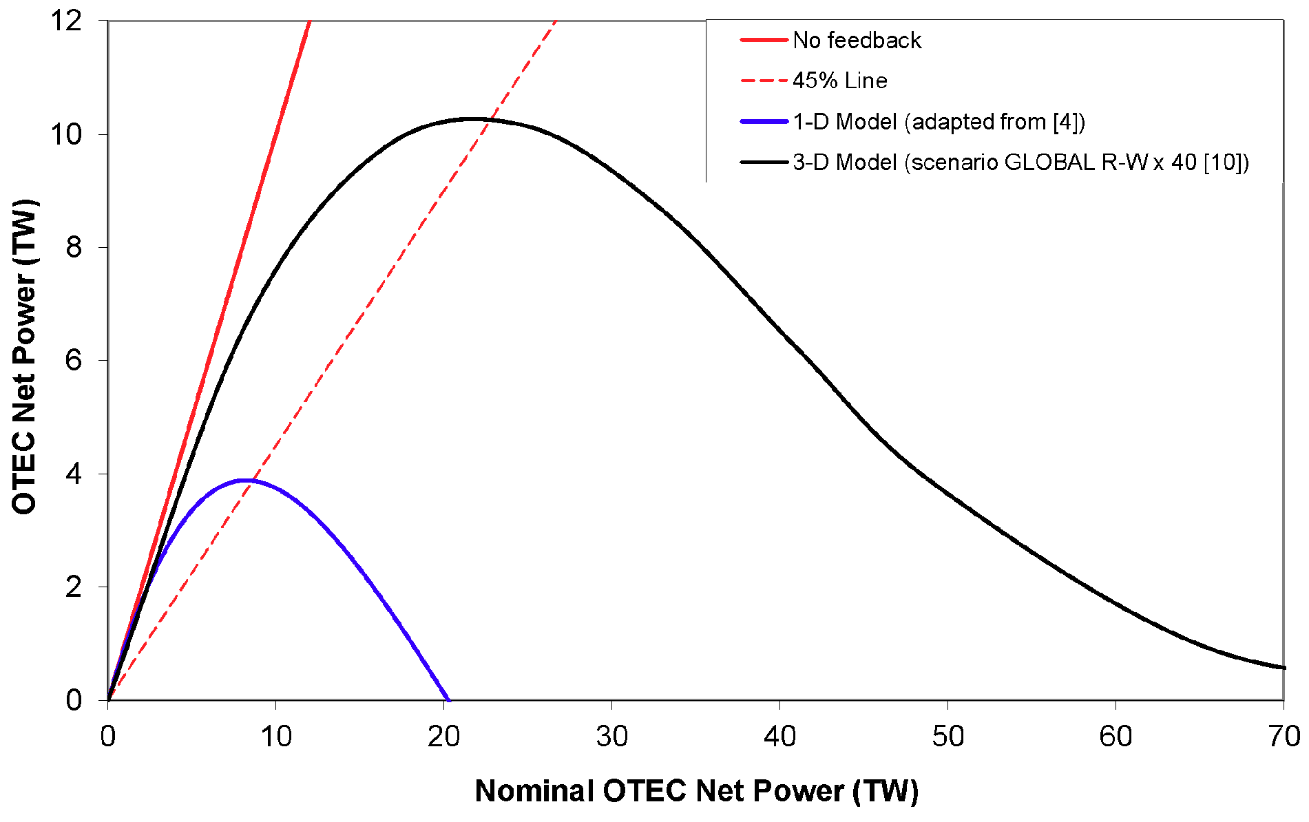
A somewhat surprising result from the much more complex analyses was that many predicted qualitative features were also apparent from the simple 1-D models, among which the existence of a steady-state (asymptotic) global OTEC net power maximum primarily caused by an accumulation of heat in the mid-depth water column. In both classes of models, and for various OTEC scenarios, the temperature profiles in the OTEC region, at maximum net power output, share many similarities, including, in particular, the amount of warming around the deep cold seawater intake depth in the OTEC region. As a result, maximum OTEC net power essentially remains proportional to deep seawater intake flow rate (or equivalently, nominal OTEC power, if there were no seawater temperature changes), with a value of the order of 0.20 TW Sv
−1 (one terawatt is 10
12 W, and one sverdrup is 10
6 m
3 s
−1); this also corresponds to a net power ratio of about 45% (i.e., power produced over nominal power). What mainly differentiates the ‘bulk’ output from all models and scenarios so far is the magnitude of the overall OTEC deep cold seawater flow rate at which OTEC net power would peak. In one-dimensional models, it basically takes much smaller OTEC seawater flow rates to modify the existing seawater temperature profiles. These points can be appreciated in
Figure 1, where the output of the most basic steady-state 1-D model has been adapted ‘locally’ to every 1 degree by 1 degree (latitude-longitude) cell of the OTEC region [
4]; the precise definition of the OTEC region, as well as the OTEC warm-to-cold seawater flow rate ratio (1.5 here, instead of 2) and net power formula were adapted for comparison to the most recent 3-D study [
10].
What all large-scale OTEC studies to date have shared is the protocol for effluent discharge. The initial 1-D analyses called for a mixed-effluent discharge at a water depth where the released water would be neutrally buoyant in the unperturbed ocean (i.e., without temperature changes) [
4,
5]. No rationale was explicitly given. The same discharge method was used in the more elaborate 3-D work, although it was recognized that an actual effluent discharge would likely occur in shallower waters, but that the ensuing plume effects (sub-grid sinking and turbulent mixing) could not adequately be captured in the ocean general circulation model at selected grid resolutions [
7,
8]; this also was consistent with running the numerically less intensive hydrostatic version of the 3-D code, where the vertical momentum equation is reduced to a hydrostatic balance. In a later study, the discharge protocol was described as a choice “with little loss of generality [
9]”, which may well turn out to be an incorrect statement.
While care was taken to avoid plume effects with OTEC effluents, other studies were conducted with similar modeling tools to investigate artificial upwelling, where convective mixing cannot be avoided since denser water is brought to shallower depths by design [
11,
12]. Even though the same caveats would apply, it was demonstrated at least that stable steady-state temperature profiles are obtained following artificial upwelling (while convective mixing schemes are used for transient calculations). Therefore, there is little reason not to contemplate alternative OTEC effluent discharge scenarios, at least from a steady-state (sustainable) perspective. This allows, in particular, the consideration of what is believed to be the most practical OTEC effluent discharge scenario, i.e., within (or just below) the oceanic mixed layer [
13]. Also, the option of locating the OTEC condenser and the cold seawater ducting at depth has been proposed for some time [
14,
15,
16], to eliminate the need for a large and costly pipe extending from the cold seawater withdrawal depth to the surface. Although detailed designs are lacking for such a concept, with serious engineering challenges of its own, implementing OTEC with a deep condenser certainly would require the cold effluent discharge to be treated separately.
The preliminary analytical evaluation of alternative OTEC effluent discharge schemes described below is based on a simple but numerically efficient 1-D algorithm [
4]. The model, described in
Section 2, is an extension of the published version that allows the possibility of separate OTEC evaporator and condenser discharges. Results are given in
Section 3, where on one hand, mixed and separate OTEC discharges are compared, and on the other hand, more practical cases of mixed or evaporator effluent discharges in shallow water are also considered.
2. One-Dimensional Steady-State Model of the Water Column with OTEC
As mentioned in
Section 1, a vertical one-dimensional steady-state model of the water column was previously used to evaluate large-scale OTEC resources [
4]. Symbols used in describing this model and its present extension are listed in
Appendix A. A diffusion-advection equation for seawater temperature was solved from the seafloor (
z = 0) to the base of a mixed layer of thickness
hm (
z =
L). The OTEC process was represented by two sinks, in the mixed layer (warm seawater intake) and at
z =
zcw (cold seawater intake), as well as by a source at
z =
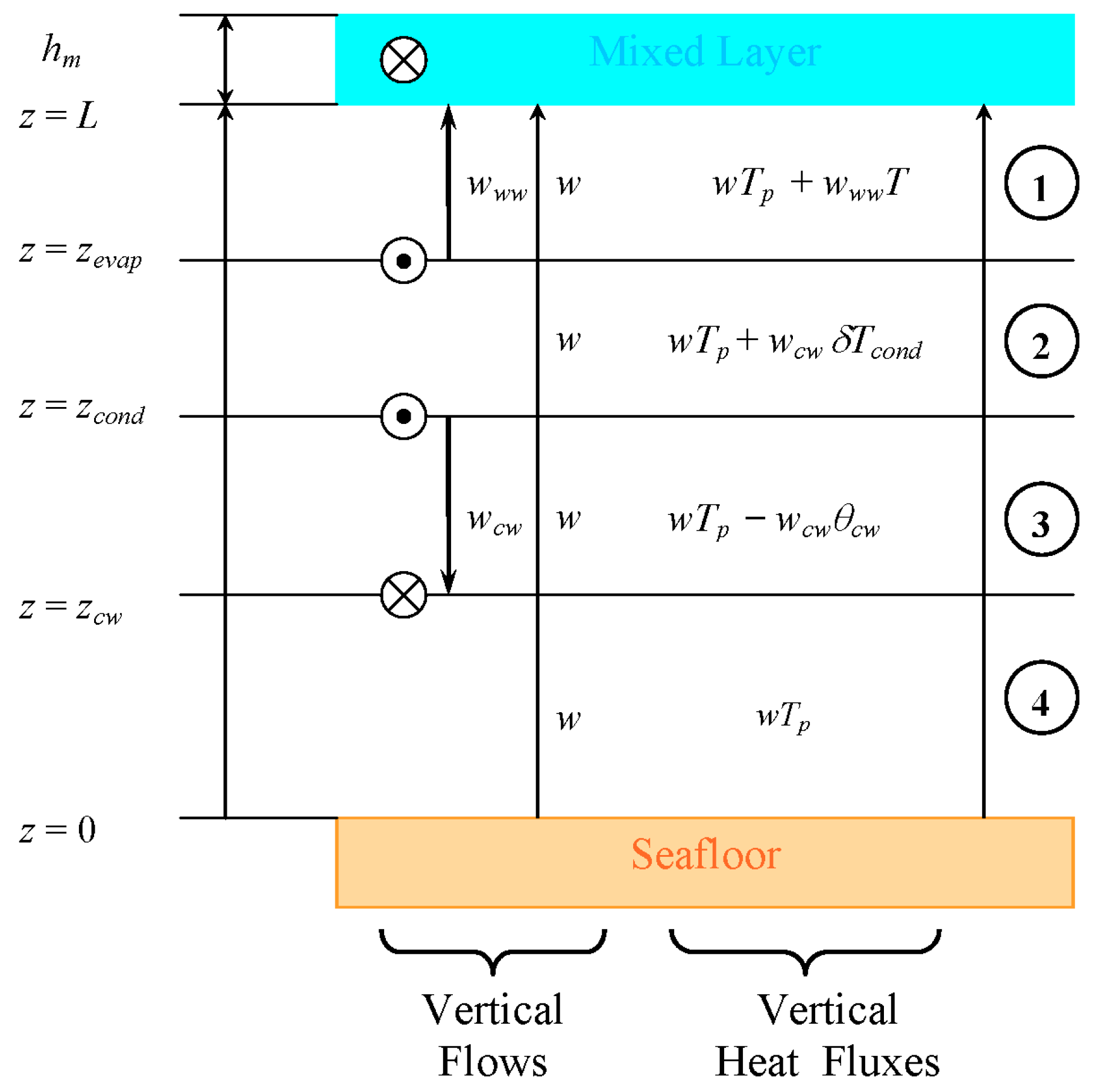
zmix (mixed effluent discharge). The present study extends the model to cases of separate OTEC evaporator and condenser effluent discharges, at
z =
zevap and
z =
zcond, respectively. This is schematically illustrated in
Figure 2. In mathematical terms, sources (depicted as circles with a dot) and sinks (depicted as circles with a cross) are Dirac distributions centered at specific vertical locations; they are singular, but with the property that a spatial integration (across such singularities) generates known step functions. Thus, the vertical domain can be split in four regions (labeled in the right-hand-side of
Figure 2) with specific vertical mass flows, normalized by
ρAOTEC, and heat fluxes, normalized by
ρcpAOTEC. The OTEC implementation area
AOTEC is a passive parameter in this 1-D model, with an order-of-magnitude value of 100 million square kilometers (10
14 m
2);
ρ and
cp are representative values of the density and specific heat of seawater, e.g., 1025 kg m
−3 and 4000 J kg
−1 K
−1. Owing to the very low thermodynamic efficiencies of OTEC cycles, an assumption that the overall OTEC process does not remove heat from the ocean is also made (lifting such assumption can be shown to result in negligible differences). Therefore, we have
www δTevap ≈
wcw δTcond, where the positive temperature differences
δTevap and
δTcond are respectively defined by the seawater temperature of the evaporator effluent
θevap =
T −
δTevap, and by the seawater temperature of the condenser effluent
θcond =
θcw +
δTcond. Finally, please note that for the mixed layer to be in steady-state equilibrium, a heat flux
wTp (not shown in
Figure 2), where
Tp is polar water temperature, must be extracted at the domain’s presumed margins to mimic deep water formation.
The steady-state temperature profile in the water column can be determined from the following steady-state heat flux equations:
These first-order ordinary differential equations require only one boundary condition each, and can easily be solved, especially if we take the vertical diffusion coefficient
K and background upward advection velocity
w to be constant, although such an expedient choice is not necessary [
11]. Since large-scale OTEC processes do affect ocean temperatures in the water column, however, one more unknown appears in the specified right-hand-sides, i.e., the cold seawater intake temperature
θcw. A similar issue does not arise for the mixed-layer temperature
T in a one-dimensional model under the assumption that the overall OTEC process does not remove heat from the ocean. In other words, there is only one possible steady-state mixed-layer temperature, although transient cooling does occur in time-domain calculations [
5]; note that a three-dimensional model would allow permanent surface cooling in the OTEC region if surface warming occurs elsewhere [
7,
8,
9,
10]. The chosen expression for the OTEC seawater condenser warming
δTcond corresponds to the simplified OTEC temperature ladder shown in Nihous [
5],
Figure 2.
The system is algebraically closed with the boundary conditions (−
K dθ/
dz +
wθ) =
wTp at
z = 0 and
θ =
T at
z =
L, in addition to three temperature continuity conditions at
zcw,
zcond and
zevap. The published algorithm for mixed OTEC effluent discharge is recovered when
zcond =
zevap =
zmix [
4]; Region 2 in
Figure 2 merely vanishes and Equation (2) need not be considered.
Before presenting results in
Section 3, a few comments about this one-dimensional model are proposed to better understand the steady-state mixed-layer heat balance under various OTEC seawater discharge scenarios, while a few expected features of the seawater temperature profile may provide calculation check points. Firstly, by comparing Equations (3) and (4), we note that the
z-derivative of
θ is continuous at
z =
zcw across the OTEC cold seawater sink. Next, in the absence of OTEC operations (
www =
wcw = 0), the steady-state mixed-layer heat balance can be written:
where the last term in the left-hand-side corresponds to deep-water formation, and the upward heat flux from the water column (between brackets) is defined by Equation (1). With OTEC operations, and if no effluent is discharged into the mixed-layer, the steady-state mixed-layer heat balance becomes:
where the first term in the left-hand-side represents the OTEC warm seawater intake sink, and the upward heat flux from the water column (between brackets) is defined by Equation (1) as before. Comparing Equations (5) and (6) reveals that the
z-derivative of
θ at
z =
L remains the same whether
www is zero (no OTEC) or not, i.e.,
dθ/
dz(
L) =
w(
T −
Tp)/
K.
If the OTEC evaporator effluent is discharged in the mixed layer, Region 1 in
Figure 2 vanishes and Equation (1) is no longer applicable. The steady-state mixed-layer heat balance is altered as follows:
where the first term in the left-hand-side represents the OTEC evaporator effluent source, and the upward heat flux from the water column (between brackets) is now defined by Equation (2). In this case, the
z-derivative of
θ at
z =
L decreases to limit diffusive heat losses from the mixed layer and compensate for the new source of cooler water; we have
dθ/
dz(
L) = {
w(
T −
Tp) −
wwwδTevap}/
K.
Finally, in the most practical case of a mixed-effluent discharge within the mixed layer (i.e.,
zmix =
L), both Regions 1 and 2 vanish, while Equations (1) and (2) are no longer applicable. Only Regions 3 and 4 are left in
Figure 2, and only Equations (3) and (4) need to be solved. The steady-state heat balance of the mixed layer is now written:
where the first term in the left-hand-side represents the net OTEC mixed-effluent source, and the upward heat flux from the water column (between brackets) is defined by Equation (3). In this case, the
z-derivative of
θ at
z =
L further decreases to limit diffusive heat losses from the mixed layer and compensate for a net input of much cooler water; we have
dθ/
dz(
L) = {
w(
T −
Tp) −
wcw(
T −
θcw)}/
K. Mathematically, Equation (8) is equivalent to the mixed-layer heat balance for scenarios of artificial upwelling (of deep water) into the mixed layer [
11]
1, since the OTEC warm seawater source and sink contributions here cancel out.
3. Results
Equations (1) through (4) are solved subject to their boundary conditions. Since the focus here is to explore different protocols for handling OTEC seawater effluents, several input choices in the model are kept the same as in Nihous [
4]. In particular, constant values of the background diffusion and advection parameters are selected, i.e.,
K = 2300 m
2 yr
−1 and
w = 4 m yr
−1; solutions in each Region labeled in
Figure 2 then involve simple exponentials of
z and constants (or in the special case
wcw =
w in Region 3, a linear function of
z). In addition, we set
Tp = 0 °C and
T = 25 °C, and select an OTEC seawater flow-rate ratio
www/
wcw of 2. The mixed layer is 75 m thick over a water column of 4000 m, and the OTEC deep cold seawater intake is maintained at a water depth of 1000 m (
zcw = 3075 m). Variable parameters are the OTEC deep cold seawater flow rate
wcw, as well as the evaporator and condenser effluent discharge depths (coordinates
zevap and
zcond in general). Once the temperature profile for a given OTEC scenario is known, OTEC power is determined from the following formula used in earlier work [
4,
5]:
where the nominal turbo-generator efficiency
εtg is 0.85, and
T in the denominator of the bracketed expression is the absolute steady-state temperature of the mixed layer, i.e., 298.15 K.
3.1. Separate Discharges versus Mixed Discharge under Baseline Scenarios
The baseline mixed effluent discharge scenario previously adopted consisted of choosing
zmix at a water depth where the mixed OTEC effluent would be neutrally buoyant without OTEC (i.e., initially) [
4]. Given the initial temperature profile obtained in this one-dimensional model, and since there is no consideration of salinity (which would also affect buoyancy), it corresponds here to a water depth of 253 m (
zmix = 3822 m, for an initial mixed effluent temperature of 18.33 °C). This approach defines baseline OTEC effluent discharge scenarios in what follows. Accordingly, in the case of separate discharges, both evaporator and condenser effluent discharges are then assumed to be initially neutrally buoyant. This corresponds to water depths of 136 m (
zevap = 3939 m, for an evaporator effluent temperature of 22.5 °C) and 602 m (
zcond = 3473 m, for an initial condenser effluent temperature of 10 °C), respectively.
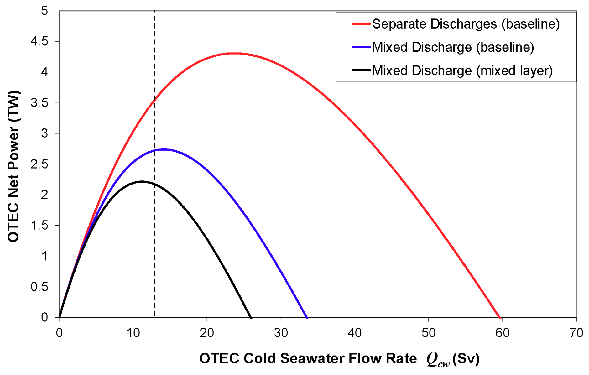
Figure 3 shows OTEC net power calculated from Equation (9), in terawatts, as a function of the overall OTEC deep cold seawater volume flow rate
Qcw =
AOTEC wcw, in sverdrups. The dotted line indicates the condition when the advective drawdown induced in Region 3 by the OTEC deep seawater intake,
wcw, is exactly equal to the background upward advection rate
w. Baseline effluent discharge scenarios correspond to the blue and red curves. It is striking that separate discharges allow a maximum OTEC net power of 4.3 TW while a mixed discharge corresponds to a value of 2.7 TW. These peak values correspond to OTEC cold seawater flow rates
wcw (
Qcw) of 7.5 m yr
−1 (23.8 Sv) and 4.5 m yr
−1 (14.3 Sv), respectively. This confirms the nearly constant OTEC seawater flow intensity at peak net power production, of the order of 0.20 TW Sv
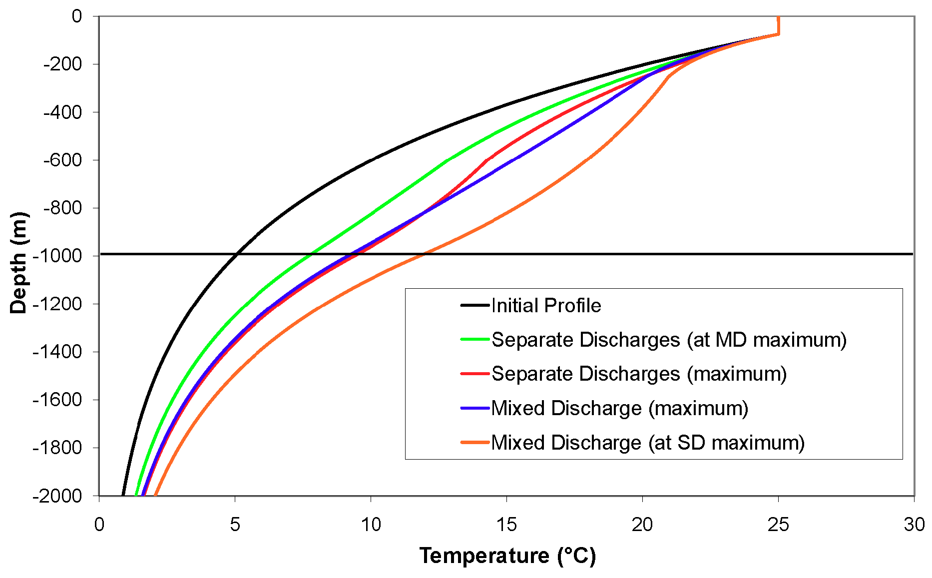
−1. It indicates, in turn, that the warming of the deep cold seawater intake temperature is nearly the same in all instances of maximum OTEC net power production. This can be seen in
Figure 4, where the blue and red temperature profiles are very similar below and across the deep-water intake depth of 1000 m. Other curves demonstrate that less degradation of the temperature profile occurs with separate discharges at given OTEC flow rates. In other words, less heat penetrates the oceanic water column across the ocean-atmosphere interface during the transient phase. This heat can be quantified by the integral
: separate OTEC effluent discharges correspond to about 60% only of the value obtained for mixed discharge.
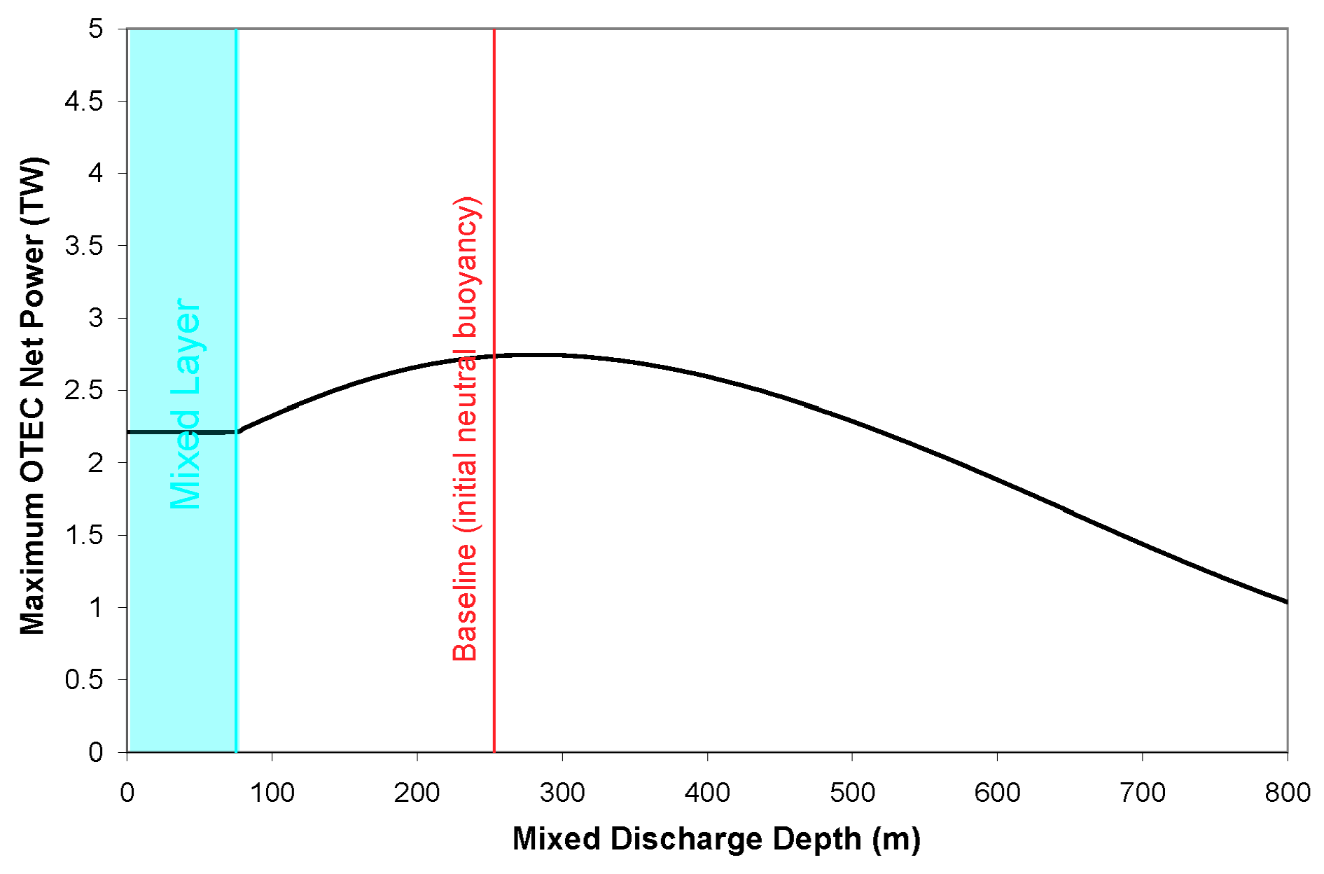
3.2. Mixed Discharge at Variable Depth
Next, mixed effluent discharge scenarios were considered at different depths, from the mixed layer downward. As noted earlier, a mixed discharge within the mixed layer may be the most practical choice from an engineering perspective, while it mathematically corresponds to an upwelling of deep cold seawater into the mixed layer.
Figure 5 shows the dependence of maximum OTEC net power as a function of mixed-effluent discharge depth. It is noticeable that the optimum choice of the discharge depth is close to the baseline value (initial neutral buoyancy). This suggests that all other things being equal, initial neutral-buoyancy of the discharged seawater corresponds to a minimal disturbance of the water column with a relatively more benign impact on the thermal structure. A discharge into the mixed layer only results in 2.2 TW, or about 80% of the baseline value. The variation of global OTEC net power as a function of overall OTEC deep cold seawater flow rate is also shown in this particular case in
Figure 3 (black curve); peak net power production corresponds to an OTEC cold seawater flow rate
wcw (
Qcw) of 3.5 m yr
−1 (11.1 Sv).
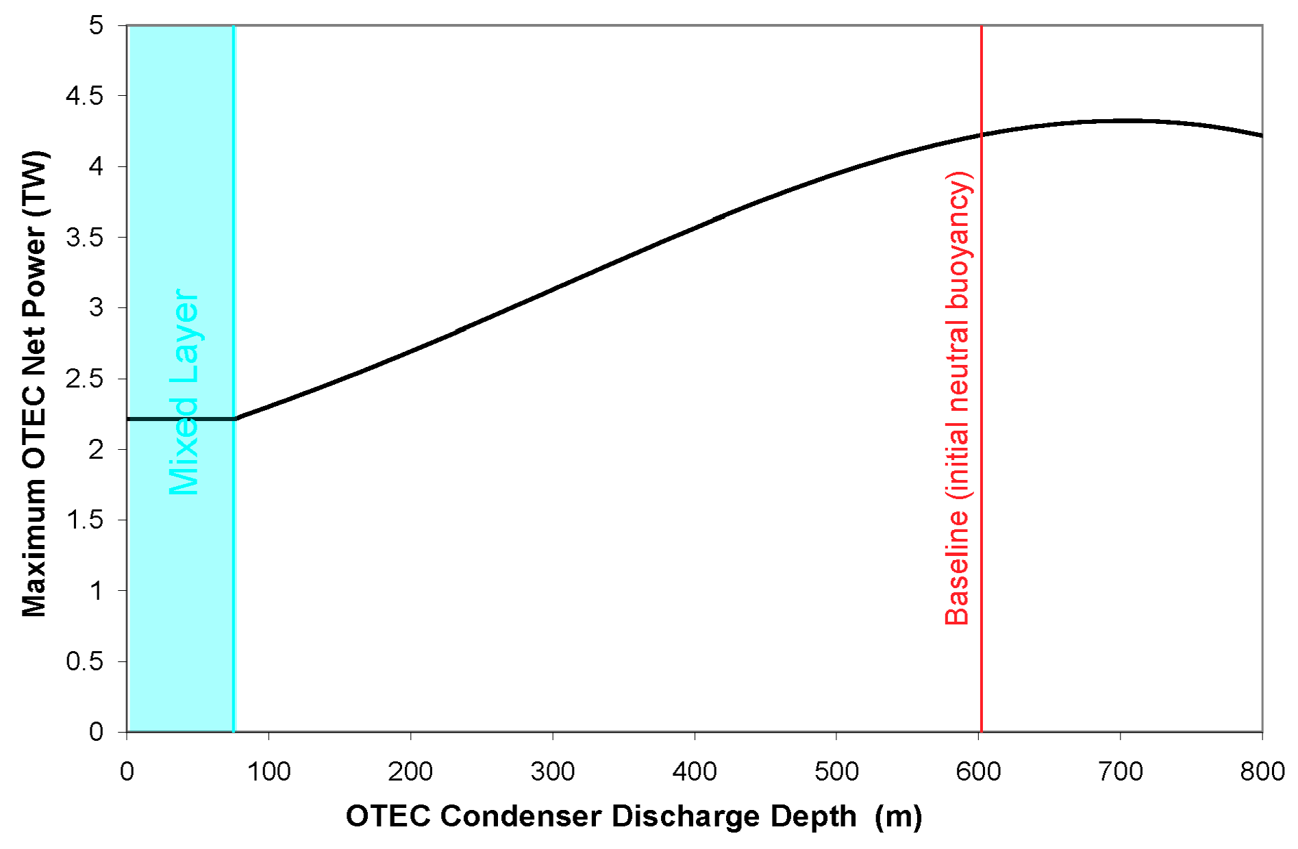
3.3. Condenser-Effluent Discharge at Variable Depth (with Evaporator-Effluent Discharge within the Mixed Layer)
Here, the effect of condenser-effluent discharge depth was examined in separate discharge scenarios.
Figure 6 shows the dependence of maximum OTEC net power as a function of condenser-effluent discharge depth, when the evaporator-effluent discharge is assumed to take place within the mixed layer. Maximum OTEC power production occurs at a condenser-effluent discharge depth of 705 m, i.e., once again, in the general neighborhood of the baseline value. Also, the peak power production, at 4.3 TW, is similar to the value obtained in the baseline scenario discussed in
Section 3.1. This indicates that the condenser-effluent discharge depth has a much greater impact than the evaporator-effluent discharge depth.
Parametric calculations where both separate discharge depths were variable yielded an overall OTEC net power maximum of 4.4 TW, i.e., hardly greater than the baseline scenario value, for evaporator and condenser effluent discharge depths of 130 m and 700 m, respectively.


