Article

Exploring Marine and Aeolian Controls on Coastal Foredune Growth Using a Coupled Numerical Model

1
College of Earth, Ocean, and Atmospheric Sciences, Oregon State University, Corvallis, OR 97331, USA
2
Deltares, 2629HV Delft, The Netherlands
3
Faculty of Civil Engineering and Geosciences, Technical University of Delft, 2628CN Delft, The Netherlands
4
Department of Geological Sciences, University of North Carolina at Chapel Hill, Chapel Hill, NC 27599, USA
5
Department of Ocean Engineering, Texas A&M University, College Station, TX 77843, USA
*
Author to whom correspondence should be addressed.
Current address: U.S. Army Engineer Research and Development Center, Coastal and Hydraulics Laboratory—Field Research Facility, Duck, NC, USA.
Current address: Van Oord, Rotterdam, The Netherlands.
J. Mar. Sci. Eng. 2019, 7(1), 13; https://doi.org/10.3390/jmse7010013
Submission received: 1 December 2018 / Revised: 21 December 2018 / Accepted: 4 January 2019 / Published: 11 January 2019
(This article belongs to the Special Issue Coastal Dune Dynamics and Management)

Abstract

:
Coastal landscape change represents aggregated sediment transport gradients from spatially and temporally variable marine and aeolian forces. Numerous tools exist that independently simulate subaqueous and subaerial coastal profile change in response to these physical forces on a range of time scales. In this capacity, coastal foredunes have been treated primarily as wind-driven features. However, there are several marine controls on coastal foredune growth, such as sediment supply and moisture effects on aeolian processes. To improve understanding of interactions across the land-sea interface, here the development of the new Windsurf-coupled numerical modeling framework is presented. Windsurf couples standalone subaqueous and subaerial coastal change models to simulate the co-evolution of the coastal zone in response to both marine and aeolian processes. Windsurf is applied to a progradational, dissipative coastal system in Washington, USA, demonstrating the ability of the model framework to simulate sediment exchanges between the nearshore, beach, and dune for a one-year period. Windsurf simulations generally reproduce observed cycles of seasonal beach progradation and retreat, as well as dune growth, with reasonable skill. Exploratory model simulations are used to further explore the implications of environmental forcing variability on annual-scale coastal profile evolution. The findings of this work support the hypothesis that there are both direct and indirect oceanographic and meteorological controls on coastal foredune progradation, with this new modeling tool providing a new means of exploring complex morphodynamic feedback mechanisms.

1. Introduction

Coastal landscape evolution reflects the aggregation of the combined effects of oceanographic, meteorological, geological, ecological, and anthropogenic influences [1]. Because of the broad range of physical processes driving temporal variability of morphology in the coastal zone e.g., [2,3,4,5], the coastal profile has often been compartmentalized into discrete morphologic units (e.g., nearshore, beach, dune) [6,7] based on dominant transport processes (e.g., waves, currents, winds). Although dunes backing sandy beaches have largely been treated as wind-controlled features, marine-driven processes play an active role in the accretional and erosional development of these landforms e.g., [8,9]. In part reflecting these complex interactions, quantitative predictions of coastal dune evolution at scales beyond individual storm events are lacking e.g., [10,11] despite the important suite of ecosystem services that coastal dunes provide (e.g., coastal protection, habitat, recreation; [12,13,14,15]).
Much of the current understanding of coastal dune evolution remains largely conceptual e.g., [2,8,11,16,17,18]. Attempts that quantify dune growth and recovery from storms come primarily from scaling up small-scale wind-driven sediment dynamics e.g., [19,20] and explorations of ecomorphodynamics e.g., [21,22,23]. Although aeolian transport is the primary driver of coastal foredune growth, in many real-world systems wind climatology is not well correlated with dune growth rates [24,25,26,27], making empirical prediction of dune evolution difficult.
The marine environment poses numerous constraints on instantaneous aeolian transport rates in sandy coastal systems, contributing to the nonlinear relationships between dune growth and climatic variables. As examples, swash-induced moisture [28], salt cementation [29], and tidally modulated groundwater tables [30] each have been found to reduce or prevent local aeolian transport. These supply limiters contribute to the widely observed fetch effect [31,32,33] whereby there is a minimum length-scale required for aeolian sand transport on beaches to reach saturation. Obliquely oriented wind results in larger effective fetch distances between the water line and the dune toe [31,34]. Oblique winds therefore will transport more sediment over the beach as compared to cross-shore oriented winds of equal magnitude in fetch limited circumstances [35]. Conversely, the cross-shore component of aeolian transport is highest under shore-normal winds and reduces with increasing obliquity, leading to a potential decrease in sediment delivery to the dune under oblique wind conditions due to the cosine effect [31]. In part due to a lack of fetch limitations [36], larger beach widths associated with low-gradient, dissipative beaches promote higher rates of aeolian transport, leading to larger dune growth relative to narrower, steeper beaches [2,8,22]. The relationship between grain size and beach slope also generally encourages higher transport rates on low sloping beaches [37,38].
Since fine grained sediment is preferentially transported by wind over coarse-grained sediment, sediment sorting and armoring may subsequently occur on mixed-grain beaches e.g., [33,39,40]—leading to complex spatial patterns in instantaneous aeolian transport. In part due to armoring effects on the upper beach, it has been found that the intertidal zone is a primary sediment source area for backshore aeolian transport [41,42,43,44]. The onshore propagation of sandbars into the intertidal zone has been recognized as a particularly important source of sediment for dune growth e.g., [26,45]. In fact, it has been hypothesized that dune growth is limited by the temporal co-occurrence of intertidal sandbar welding events with the capacity to mobilize sediment by wind [26]. However, field data from a dissipative beach have demonstrated that dune growth can occur regardless of in-phase synchronization of maximum beach sediment supply and maximum dune growth [46].
Energetic wave conditions and high water levels in the collision regime of the Sallenger [9] Storm Impact Scaling Model have often been related to the erosion of coastal foredunes e.g., [47,48]. The exposure of coastal dunes to erosion is related to a variety of morphologic and environmental controls e.g., [49,50], although low sloping, wide beaches are generally less vulnerable to dune erosion than steep, narrow beaches. It has also been recently demonstrated, using both field data [46] and numerical models [51], that infragravity swash processes can contribute directly to dune growth on dissipative beaches. These results give further evidence of the direct and indirect roles of the marine system in governing both accretive and erosive dune processes.
Despite a qualitative understanding of the dominant marine and aeolian processes controlling coastal foredune evolution, quantitative models able to reliably simulate dune growth in real-world coastal systems, including the recovery of coastal dunes following storm-induced erosion, are lacking [10,11]. Recognizing that major gaps in knowledge of sediment transport and morphological change across the land-sea interface still exist, here we introduce the coupled coastal profile modeling framework Windsurf. Windsurf couples three state-of-the-art open-source models that independently account for subaqueous (XBeach; [52]) and subaerial (Aeolis; [33]; Coastal Dune Model (CDM); [22]) processes to explore the evolution of the coastal profile in response to both marine and aeolian forcing (Figure 1). The numerical models within Windsurf are capable of simulating complex coastal behaviors such as beach growth [53], swash dynamics [54], wave-driven dune growth [51], storm-induced dune erosion [55], overwashing [56], aeolian sediment sorting [33], and ecological controls on dune growth [22]. In this paper, we aim to test this new Windsurf model coupling framework. Windsurf is used to hindcast prograding and dissipative conditions for a one-year period at a data rich field site in the U.S. Pacific Northwest (PNW). This work serves as a proof of concept of Windsurf, with the model outputs additionally used to gain new insights into the relative controls of marine and aeolian processes on coastal foredune growth.
The structure of this paper is as follows. Details of the new Windsurf modeling framework and its sub-models are described in Section 2. Morphologic and environmental field datasets used to validate Windsurf are presented in Section 3. Windsurf simulations completed for the PNW field site are described in Section 4. Discussion of the results and conclusions are given in Section 5 and Section 6, respectively.

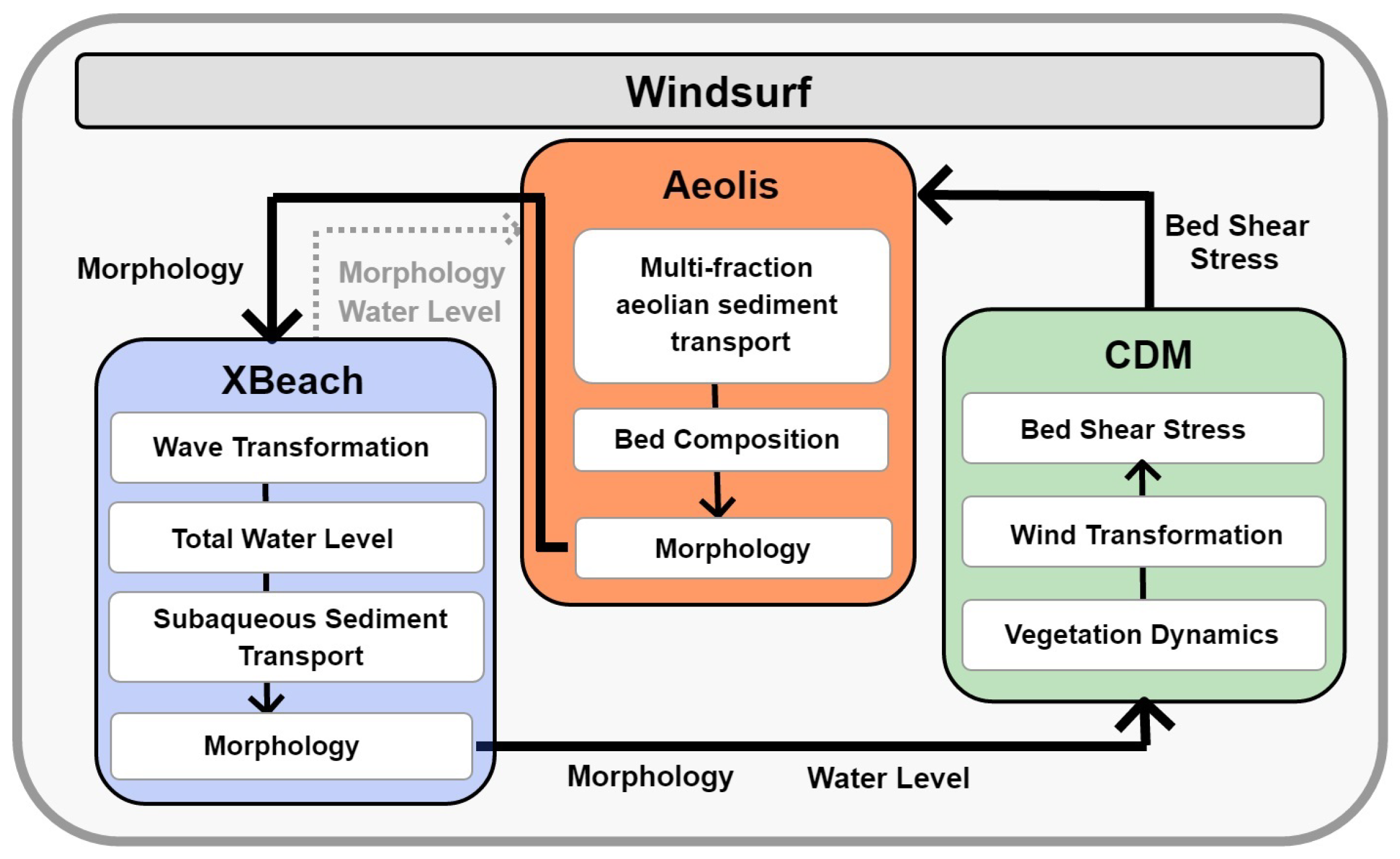
2. Windsurf Model Framework

The following section describes the details of the Windsurf model coupler, followed by details of the process capabilities of the individual numerical models within Windsurf.

2.1. Model Coupler

Windsurf couples three separate open-source numerical models [henceforth referred to as model cores] which simulate subtidal morphodynamics related to waves and currents (XBeach), subaerial morphodynamics related to wind shear and vegetation (CDM), and multi-fraction aeolian sediment transport that includes the effects of supply limiters (Aeolis) (Figure 1 and Figure 2). Together, these model cores simulate the evolution of the full coastal profile in response to both marine and aeolian forcings.
Windsurf serves as the back-end coupler to these three model cores, with functionality to generate input files, execute model simulations, exchange information between model cores, and save model output. The Windsurf framework runs the individual model cores in series, with morphological, environmental, and ecological information exchanged between the models at user-defined time steps (Figure 2). By using a loosely coupled approach in which the model cores are separated from the coupler, the individual models can continue to be developed independently and new model components can easily be incorporated into Windsurf. New capabilities can be added if the additional model core can run on or be interpolated to a central model grid. Currently, Windsurf model grids are limited to 1D, cross-shore only applications; however, extension to 2D is planned for future work.
The work presented in this manuscript uses a version of the Windsurf framework coded in MATLAB (v2017a or newer) which runs the process-based model cores in an offline mode. That is, the model cores are initialized and fully executed before moving on to the next model core. As schematized in Figure 2, Windsurf first runs XBeach to simulate marine-related processes and resulting morphology change. XBeach runs are followed by CDM which simulates spatio-temporal vegetation dynamics and the cross-shore wind field, including the effects of dune grass vegetation on bed shear stress reduction. Finally, Aeolis simulates aeolian sediment transport and aeolian-driven morphology change. A link to the Windsurf model coupling code can be found in the Supplementary Materials.

2.2. XBeach

XBeach is an open-source process-based numerical model which simulates nearshore wave transformation, subaqueous sediment transport, and morphology change [52]. XBeach has been used in numerous studies investigating wave transformation [57,58], swash processes [46,54,59], and morphology change [55,56,60,61,62]. Originally developed for assessing impacts from discrete storm events, the model has more recently been applied to simulate marine-driven morphologic changes on time scales of weeks to years [53,63,64]. An overview of relevant processes and model parameters for XBeach are described below, while a full description of the model and its formulations can be found in Roelvink et al. [52] and Roelvink et al. [65].
When using XBeach in surfbeat mode, the model does not resolve individual short waves but does resolve the wave group envelope using the time dependent, short-wave action balance equation [52,66]. The short-wave action balance equation is also coupled with the nonlinear shallow water equations to account for infragravity waves and mean currents. XBeach, which is a depth-averaged model, solves these spatially varying hydrodynamic processes in either 1DV (cross-shore profile model) or 2DH (area model).
Sediment transport is solved by an advection-diffusion equation [67]. In surfbeat mode, as XBeach is presently applied in the Windsurf framework, wave groups are resolved but individual incident (short) waves are not modeled. As the wave shape is not directly simulated, the effect of wave nonlinearity on sediment transport is parameterized via the short-wave-related velocity asymmetry (facAs) and skewness (facSk) coefficients. Many studies provide guidance on the effects of facAs and facSk on simulating erosional and accretional processes with XBeach e.g., [68,69,70]. Mean currents and long waves also contribute to sediment transport. Spatial gradients in the short-wave and current related sediment transport rates simulated by XBeach are used to calculate the resulting bed level changes using a form of the Exner equation. McCall et al. [56] found that morphology change associated with overwash and other high flow currents are often overpredicted. To address this issue, the dilatancy option accounts for the influence of pore water on bed stability, effectively increasing the local critical Shields parameter and thereby reducing transport rates during high flow conditions following the methods of van Rhee [71]. A morphologic acceleration factor (morfac) can also be implemented in XBeach according to the methods of Reniers [72]. Morfac allows morphology change to be scaled, enabling shorter duration numerical simulations without significant loss in process resolution e.g., [68,73].

2.3. Coastal Dune Model

The CDM can simulate the evolution of vegetated coastal foredunes by solving a suite of differential equations describing ecomorphodynamic processes [22]. The model originated as a 1D dry-environment saltation model [74] to simulate the formation and migration of desert dunes. Later work extended the model to a 2D area model and added the role of vegetation in stabilizing the dune form [75]. The model has been used to explore the formation mechanisms and time scales of linear [76], parabolic [75], and barchan [77] dunes. The latest iterations of CDM have been applied to simulate controls on coastal foredune ridge development [78], post-storm dune recovery on barrier islands [79], and controls on foredune hummockiness [80]. A key driver of these different morphological forms is resolving the feedback of the topographic field on the local wind field. The computationally efficient wind model of Weng et al. [81] that is implemented in CDM builds upon Hunt et al. [82], an analytical solution for turbulent shear flow over a low sloping hump, to solve for the spatially variable bed shear perturbation field ( δ τ ) on the beach and dune.
In addition to resolving wind and aeolian transport dynamics, CDM tracks the spatial and temporal growth of dune vegetation by assuming a linear growth rate of the vegetation cover fraction ( ρ v e g ; [22]). The effective bed shear stress ( τ s ) in the presence of vegetation, which is calculated by CDM, becomes:
τ s = τ o + τ o δ τ 1 + m β σ ρ v e g
where τ o is the bed shear stress in the absence of variable topography or vegetation, m is the vegetation friction coefficient, σ is the ratio of the plant basal to frontal area, and β is the ratio of the plant drag coefficient to bare sand [83].
CDM has the capability to simulate aeolian sediment transport using the derived bed shear stress field. The model assumes a single (spatially constant) grain size and has shown success in simulating coastal dune dynamics in a variety of morphodynamic settings e.g., [22,78,80]. When forced with cross-shore directed winds, CDM model results have suggested that LVeg, defined as the distance between the shoreline and the perennial vegetation line, can exert a primary control on the maximum height which dunes can grow [22]. Since the shoreline position is typically non-stationary in real-world settings, in Windsurf LVeg is modified to allow for vegetation growth that follows a fixed vertical contour position rather than a fixed beach width. That is, as beaches and dunes erode or prograde, the seaward-most location of vegetation in the model is assumed to follow the seaward-most location of a fixed vertical contour rather than remain at a fixed horizontal position. Furthermore, to allow for obliquely oriented winds in Windsurf, the cross-shore oriented CDM grid is rotated at each coupling time step based on the wind direction to properly resolve the δ τ field over the foredune. Within Windsurf, CDM is used to compute the spatially varying topographically and ecologically influenced bed shear stress field. CDM is not used directly for aeolian transport calculations within Windsurf in part because only a single grain size can be implemented in the model. Instead, using the CDM calculated spatially variable bed shear stress field, multi-fraction aeolian sediment transport is simulated using Aeolis within the Windsurf framework. For additional information on CDM and its formulations see Durán and Moore [22], Moore et al. [78], Durán and Moore [79] and Goldstein et al. [80].

2.4. Aeolis

Aeolis is an aeolian sediment transport model specifically designed to simulate supply limiting processes [33,84]. As wind processes entrain and transport sediment via saltation, the model accounts for the temporal and spatial evolution of the grain size distribution at the bed surface, and with depth, on either a 1D (cross-shore) or 2D domain. Within each model grid cell, local wind properties (bed shear stress and wind velocity) are used to calculate sediment transport rates for each grain size bin ( d n ). The saturated sediment mass-flux transport rate ( q s a t ) is calculated for each d n based on the formulation of Bagnold [38]:
q s a t = C b ρ a g d n D n u * - u * t h 3
where ρ a is the air density, D n is a reference grain size of 0.25 mm, u * is the shear velocity, u * t h is the threshold shear velocity below which transport does not occur, and C b is an empirical coefficient. The shear velocity threshold for transport is calculated via Bagnold [38] and modified incorporating the effect of moisture following Belly [85] ( f m ):
u * t h = f m A ρ s - ρ a ρ a g d n
where ρ s is the sediment density and A is an empirical coefficient. For the present application moisture-related effects ( f m ) are only used in the swash zone to limit aeolian transport in the presence of high water levels; precipitation and groundwater–related moisture are not yet implemented in Windsurf but will be accounted for in future versions. A weighted saturated sediment concentration is calculated using the local bed grain size distribution. Sediment transport gradients, resulting from local sediment characteristics, supply limiting effects (e.g., moisture, salt content), and/or the spatially variable wind field, produce local bed elevation changes.
The Aeolis model has shown skill at simulating complex sediment sorting and beach armoring processes [33]. Because of the added capability of simulating multi-fraction aeolian sediment transport and the inclusion of other supply limiting effects, Aeolis is used as the subaerial transport model within Windsurf. Windsurf provides Aeolis with spatially varying wind and bed shear stress fields from CDM and the total water level from XBeach at each time step. Aeolis is run using the full bed shear stress derived from CDM to calculate aeolian sediment concentrations which are advected using only the cross-shore component of wind field for the 1D Windsurf simulations described in this manuscript. For additional information on the details of Aeolis, see Hoonhout and de Vries [33].

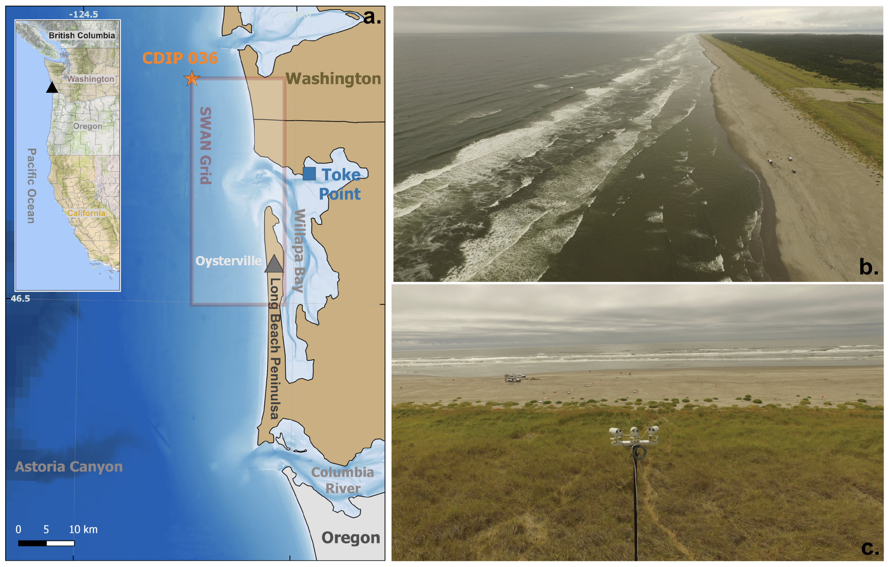
3. Field Observations at a Prograding Coastal System

To test the ability of the new modeling framework to simulate realistic behavior, Windsurf is applied to a prograding coastal field site in the PNW. The following sections briefly describe the field site and the relevant datasets for model implementation.

3.1. Field Setting

The Long Beach Peninsula, WA (LBP; Figure 3) is a modally dissipative, mesotidal (2–3 m tidal range) coastal system in the PNW characterized by low-gradient (backshore slopes of ∼0.025), sandy beaches, and linear foredune ridges densely colonized with Ammophila breviligulata (American beach grass; [21,86]; Figure 3b,c). In the Oysterville section of LBP, the beach is rapidly prograding (>4 m/year) in response to gradients in longshore sediment transport and cross-shore sediment feeding from the shoreface [7]. The dune complex is also prograding, with approximately 10–15 m 3 /m/year of dune growth [46] which contributed to the generation of a new foredune (the seaward-most dune) since the late 1990s [78]. The dune crest elevation at Oysterville is about ∼9 m NAVD88, corresponding to about 7 m above mean high water (MHW, 2.1 m NAVD88).
Long-term dune growth at this site is driven primarily by wind-driven processes [46]. The outer Washington coast is characterized by a seasonal wind climate, with the largest average monthly wind speeds in January and December. The highest wind speed events typically co-occur with large wave events. While high total water levels (TWLs), driven in part by large wave heights, regularly impact the dune toe at Oysterville, WA, previous observational [46] and modeling [51] studies have indicated that these TWLs may also directly contribute to growth of the lower portion of the dune at Oysterville.
High TWLs at Oysterville are primarily a result of large wave runup associated with an energetic wave climate in the PNW. The average deep-water winter significant wave height (H s ) offshore of the PNW is about 2.3 m, with numerous storms each year exceeding 8 m [86]. These high energy conditions seasonally erode the foreshore, leading to oscillations of the MHW shoreline of over 30 m despite a net annual progradation of the system [86,87]. Beach recovery occurs predominantly in the low energy summer period (H s ∼1.5 m on average) in response to the onshore propagation and welding of intertidal sandbars [46,88].
The surf zone at the study site is typically characterized by numerous (2–4) subtidal sandbars which vary significantly on interannual time scales [89] as captured by a coastal monitoring program that has been ongoing since the late 1990s [86]. Recent work has focused on characterizing sub-annual coastal evolution at Oysterville [46,88]. The existence of morphology data at a wide range of time scales at a site with large morphology change signals makes Oysterville an ideal location to test the new Windsurf modeling framework.

3.2. Morphology Data
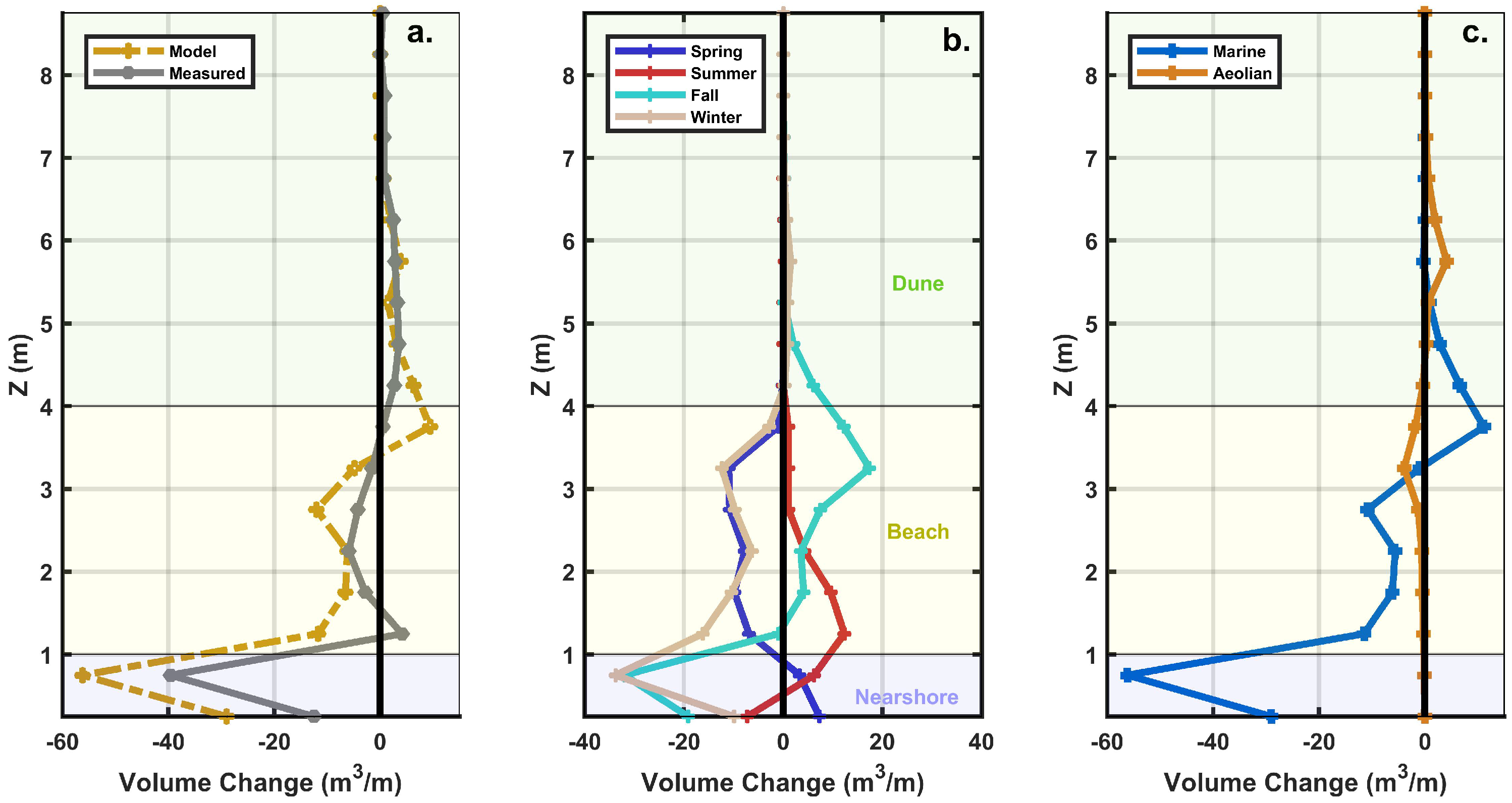
3.2.1. Annual Scale

Topographic and bathymetric measurements have been made at Oysterville using real time kinematic GPS surveying techniques [86]. A single cross-shore transect that extends from 9 m water depth to landward of the foredune crest is used here. The measured cross-shore transect data are used for input to the numerical model and for comparison to model output. From these data, volumetric changes were calculated between morphological units, where the nearshore is defined here as the region from −9 to 1 m NAVD88 [all vertical references henceforth are relative to NAVD88]. The upper limit of the nearshore zone corresponds approximately to local mean sea level at the field site. The beach is defined here to be between the 1 m and 4 m contours and the dune region includes all areas above the 4 m contour, where 4 m is the approximate dune toe position. Measurements between 4 August 2016 and 9 August 2017 show nearshore ( Δ V n e a r s h o r e ), beach ( Δ V b e a c h ), and dune ( Δ V d u n e ) volume changes of −166 m 3 /m (∼±300 m 3 /m), −5.4 m 3 /m (∼±13 m 3 /m), and 16.7 m 3 /m (∼±5 m 3 /m), respectively (Figure 4 and Figure 5). Please note that the listed volumetric change uncertainties are calculated by combing the random vertical uncertainties associated with topographic (∼8 cm; e.g., [86]) and bathymetric (∼13 cm; e.g., [90]) field measurements in quadrature.
The data show that on annual scale there is variability in the subtidal sandbar configuration (Figure 4). The net sediment loss from the nearshore that was not gained by the beach reflects either longshore gradients in transport or large errors associated with volumetric estimation from bathymetric data. Between the two profile measurements, there was also a net 10 m retreat of the MHW shoreline ( Δ X M H W ), with this apparent shoreline change occurring in part because of configurations of intertidal sandbar troughs at the time of the surveys (Figure 4). This indicates that despite measured dune growth at the site, there was effectively no net beach change over this particular year (within the error of the instrumentation).

3.2.2. Sub-Annual Scale

An additional 9 topographic surveys were completed between the August 2016 and August 2017 survey dates which are also used to inform the timing and magnitude of beach and dune morphology changes at sub-annual scale. Details of the morphology change on these time scales, using data from the same field site, are described in Cohn et al. [46]. Because MHW shoreline change is often used as a metric for coastal change e.g., [91], temporal changes in the MHW shoreline are also extracted from the data (Figure 5a). These data show that between the August 2016 and August 2017 profile there is seasonality in the beach behavior. The beach was widest in summer (July–September) and fall (October–December) and narrowest in winter (January–March) and spring (April–May), with about 40 m variability in Δ X M H W over the full year. Volume changes in the beach and dune are also calculated at this monthly time scale (Figure 5b,c). Δ V b e a c h has the same seasonal behavior as Δ X M H W . Conversely, the dune shows gradual volumetric growth throughout the year. The dune volume increases or remains constant between each survey (within the measurement uncertainty), with the lowest rates of dune growth occurring in summer.

3.3. Environmental Data

3.3.1. Water Levels

Offshore waves and still water levels (SWL) are the primary drivers of marine-driven morphology change and therefore serve as important model boundary conditions. A Nortek Acoustic Wave and Current Profiler (AWAC) was deployed on a bottom mounted mooring at −9 m providing wave and SWL measurements for a 42-day period during summer 2016 as part of the Sandbar Aeolian Dune Exchange Experiment (SEDEX 2 ) [88]. To temporally extend the record of oceanographic forcings at the study site beyond the SEDEX 2 period, additional nearby measurements from the U.S. National Oceanic and Atmospheric Administration (NOAA) Tides and Currents database, the U.S. National Data Buoy Center (NDBC), and the Coastal Data Information Program (CDIP) are used.
The AWAC-derived SWLs show similar tidal amplitudes (Figure 6a) as compared to measurements from the NOAA Toke Point, WA tide gauge located 20 km to the northeast of Oysterville in Willapa Bay (Figure 3a). Slight (≤1 h) tidal phase offsets between the sites contribute to a root mean square error (RMSE) of 0.29 m between the AWAC and Toke Point SWLs for the SEDEX 2 period. For modeling purposes, hourly tidal measurements from Toke Point, WA are used directly.

3.3.2. Waves

Offshore wave information, including significant wave height (H s ), peak wave period (T p ), and wave direction (D w a v e ), were acquired from CDIP buoy 036, located 35 km to the northwest of the study site in 40 m water depth (Figure 3a). The SWAN model [92] was used to transform waves from the CDIP buoy to the AWAC location. A 2D SWAN grid (dx = 100 m, dy = 100 m) that encompasses the northern half of LBP (Figure 3a) was set up using a regional, high resolution NOAA [93] bathymetric digital elevation model to define the offshore water depths. Standard PNW model configurations e.g., [94] are used for this application. Local wind wave generation was neglected.
SWAN was used to transform waves to the AWAC location for each hour between August 2016 and August 2017 using the CDIP 036 measured H s , T p , D w a v e and the tide gauge measured SWL (Figure 6b–d,h–j). SWAN performs well at modeling wave transformation to Oysterville, with minimal bias ( Δ μ ) and RMSEs of 0.12 m, 1.7 s, and 8.0 for H s , T p , and D w a v e , respectively, relative to the AWAC data (Table 1; Figure 6b–d).

3.3.3. Wind

For the period between 3 August 2016 and 21 May 2017 a Dyacon MS-140 weather station was deployed on the foredune crest at the Oysterville site and provided bulk wind speed (u) and direction (D w i n d ) measurements. To extend the meteorological measurements beyond this local measurement period, available wind data from the NOAA Toke Point wind gauge were used. First, both datasets were transformed to their 10 m equivalent wind speeds. Then a linear transformation function was developed to relate u and D w i n d from Toke Point, WA to Oysterville, WA using the overlapping time series. The transformation generally agrees well with local wind speed data (Figure 6e), with a RMSE for the locally predicted wind speed of 1.13 m/s with a small Δ μ (−0.37 m/s). However, there are periods when wind direction is poorly resolved, likely because of the local topography within Willapa Bay. Therefore, while 77% of the locally transformed D w i n d are within ± 5 of the measurements, there is a fairly high overall RMSE value of 25.5 for the wind direction transformation (Table 1). Because local wind measurements were made for 78% of the full year simulation period, the transformed data was used only when local measurements were not available.

4. Hindcast Simulations

Windsurf was applied to the Oysterville, WA field site. The following sections describe the procedure for model parameter calibration for a one-year simulation period and present the results of the calibrated case.

4.1. Windsurf Calibration

4.1.1. Model Setup

To calibrate Windsurf to Oysterville, a set of model simulations were initialized with the measured topographic and bathymetric profile from 4 August 2016 and run for a one-year period (until 9 August 2017) using the locally transformed SWLs, waves, and winds described above. A one-hour model coupling time step between the model cores was used, commensurate with the availability of oceanographic and meteorological forcing data and to adequately resolve processes on the intra-tide time scale. Within CDM the lower vertical limit of perennial vegetation was set to be 5.5 m based on local field observations (Figure 3b,c). CDM was initialized with spatially uniform vegetation ( ρ v e g = 1) above this elevation.
A locally measured grab sample was used to inform the grain size (D50 = 0.25 mm, D90 = 0.335 mm) input to Windsurf. In the absence of detailed spatio-temporal grain size data at the field site, the grain size distribution is assumed to be spatially constant in both XBeach and Aeolis.
The 1D cross-shore model grid has variable grid spacing between 20 m (offshore) and 2.5 m and encompasses the region from –9 m to landward of the foredune crest. It is important to note that during energetic wave conditions wave breaking occurs deeper than the –9 m depth, inducing sediment transport near the offshore boundary and imposing implications on the incoming infragravity wave field. It was not practical to extend the model grid to significantly deeper water depths for this application. Therefore, consistent with the bathymetry observations (Figure 4) it was assumed that at the cells near the offshore model boundary (−9 m) there is no net bed level change on the time scales of interest. Any XBeach simulated sediment losses in this region are assumed to be replenished by either cross-shore feeding from the shoreface and/or longshore transport gradients. No modifications are made to modify the incoming bound long wave field, but it is assumed that infragravity generation within the inner surf zone from active wave breaking is of first order importance over far-field infragravity generation mechanisms for this model application.

4.1.2. Calibration Procedure

Process-based numerical models, including each Windsurf model core, typically have several tunable, site-specific parameters representing unknown model physics or site-specific transport properties e.g., [68,95]. Following preliminary model core sensitivity testing, four specific model parameters were identified for further exploration: the short-wave-related asymmetry (facAs, XBeach) and skewness (facSk, XBeach), the aeolian sediment transport coefficient (Cb, Aeolis), and the vegetation friction coefficient ((m, CDM). A choice of one year for model calibration was specifically chosen to ensure that the model is not biased towards simulating only accretional or erosional processes, as Oysterville has significant seasonal morphological variability (Figure 5).
As has been previously noted, XBeach is particularly sensitive to choices of facAs and facSk e.g., [68,69,70]—often requiring separate parameter combinations for accretional and erosional conditions e.g., [53]. Preliminary model core testing (not shown) did not yield realistic behavior when using constant facAs and facSk for the full year period. Therefore, following the general methods of Pender and Karunarathna [53], different model parameter combinations for these two variables were calibrated for low energy (assumed to be when H s ≤ 2 m for our purposes) and high energy (H s > 2 m) conditions. When H s is below this 2 m threshold, field observations show that intertidal sandbars are typically observed to move onshore at the field site [88]. Above this wave height threshold, intertidal sandbars are generally eroded at Oysterville [46].
To calibrate Windsurf to the field site, a set of one hundred year-long Windsurf simulations were completed using random combinations of m, Cb, facAs (low energy), facAs (high energy), facSk (low energy), and facSk (high energy) (see Table 2 for range of values). Each of the 100 simulations were identical other than these parameter settings. Beyond this, typical model parameter settings are used for all three model cores. Please note that for XBeach a morfac of 2 was used and the dilatancy option was turned on.
Differences between the measured and modeled Δ V s u b a e r i a l ( Δ V b e a c h + Δ V d u n e ) were calculated at 10 time intervals (9 monthly surveys and the final August 2017 survey) from all 100 Windsurf simulations. The locally calibrated (best-fit) simulation was defined as the model simulation with the lowest RMSE Δ V s u b a e r i a l as calculated from all 10 Δ V s u b a e r i a l error estimates. This calibration approach was designed with the overall aim of discerning the relative controls of marine and aeolian processes on coastal foredune evolution. While calibrating the model to the monthly volumetric change data ensures that the model simulates realistic coastal profile changes at Oysterville, this exercise does not imply that Windsurf is validated to explore all coastal behaviors or for other sites e.g., [96,97].

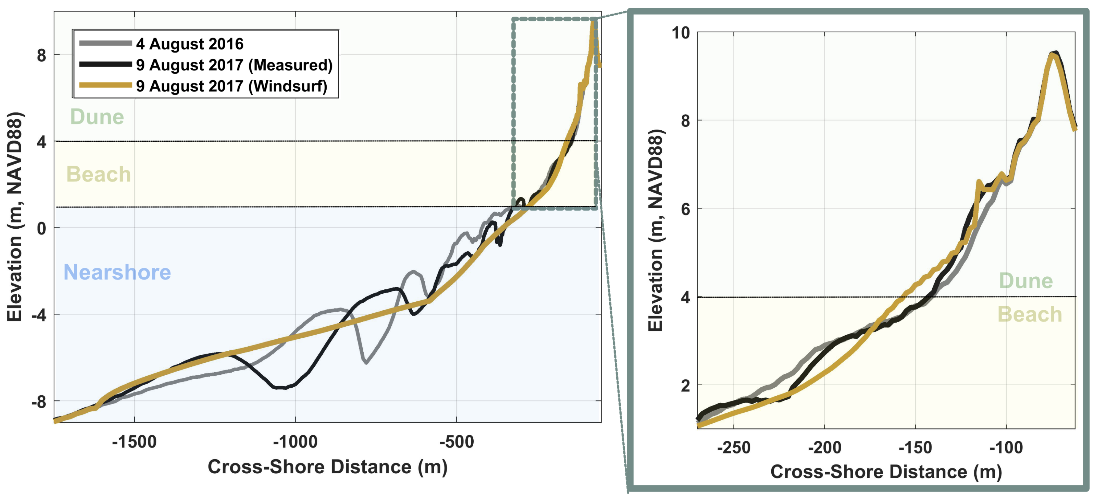
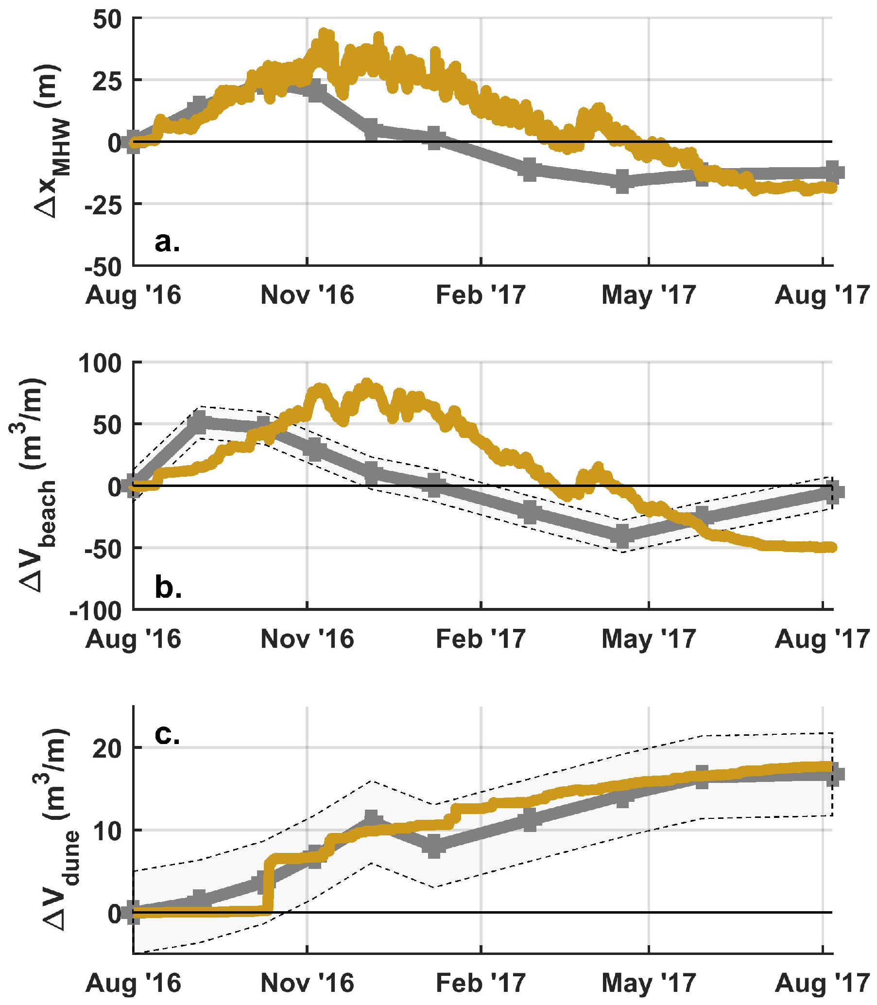
4.2. Calibrated Model Results

The results from the best-fit calibrated simulation for Oysterville, WA between August 2016 and August 2017 are shown in Figure 4. Qualitatively, the simulated profile matches the field measurements, with growth of the dune and modest net changes to the beach modeled after one year. However, the model does not accurately reproduce the changes to the subtidal sandbars (Figure 4). Both subtidal and intertidal sandbars are smoothed during the simulations by XBeach (and potentially the other model cores).
In response to low wave energy conditions in summer, Windsurf simulates beach progradation by up to 44 m at the MHW shoreline (Figure 5). The widest beach state is modeled to occur in early November. Thereafter, the simulation shows gradual retreat of the MHW shoreline until May 2017. The shoreline remains relatively stable (±5 m) from May until the end of the simulation in August 2017. The beach volume changes track the same general temporal behavior as Δ X M H W . A total of 17.7 m 3 /m/year of dune growth is simulated compared to the field measured Δ V d u n e of 16.7 ± 5 m 3 /m over the year.
Outputs from each model time step are used to investigate the relative contributions of marine and aeolian processes to coastal profile change and to explore the timing of depositional and erosional processes. The outputs are binned into 0.5 m vertical increments as shown in Figure 7, with these bins corresponding to the vertical elevations of the initial (4 August 2016) profile. In vertical cross-section, the numerical model results show reasonable agreement with the measured data over the annual scale (Figure 7a). Volumetric changes in the inner nearshore, between the 0 m and 1 m contours, are erosional in both the model and the observations. The model simulates more erosion around the 3 m contour and more deposition around the 4 m contour than revealed by the observations, although the model successfully reproduces the deposition of sediment between the 5.5 m and 7 m contours (Figure 4 and Figure 7a).
Windsurf simulates that growth of the lower portion of the beach (∼1–2 m elevations) is largest in summer, in agreement with the observations (Figure 7b). The largest upper beach growth (∼2–4 m elevations) instead occurs in fall, while the largest beach losses occur in winter. Although there is relatively little ( Δ V b e a c h <30 m 3 /m) net change to the beach compartment over the year, the seasonal fluctuations in beach volume growth are significantly larger than volumetric variability within the dune region. The largest volume gains to the dune occur in the fall (10.3 m 3 /m), followed by winter (4.4 m 3 /m), spring (2.4 m 3 /m), and summer (0.6 m 3 /m).
As Windsurf computes dz related to marine transport by XBeach and aeolian transport by Aeolis at each coupling time step, it can be determined which volumetric changes across the profile can be attributed to marine versus aeolian processes, as shown in Figure 7c. The Windsurf simulations suggest that there are both marine (10.1 m 3 /m/year) and aeolian (7.6 m 3 /m/year) contributions to dune growth above the dune toe. Most of the marine-driven deposition to the dune is simulated near the 4 m contour—the approximate dune toe for the region. Above the 6 m contour, where swash did not frequently reach, all the simulated deposition (3 m 3 /m/year) is from aeolian processes.
These results suggest that marine-driven dune accumulation at 4 m or above occurs primarily during high SWL events and/or during periods of large wave energy (elevated H s and/or T p ; Figure 8a–c,f–h). Although most environmental conditions show positive Δ V d u n e , small (<0.1 m 3 /m) negative Δ V d u n e are occasionally simulated (e.g., T p of 19 s; Figure 8c) indicating that marine processes also drive dune erosion at this site under some forcing conditions. There are fewer environmental limiters on aeolian-driven dune growth (Figure 8), although the largest contribution to dune growth occurs from oblique or alongshore winds from the south (Figure 8e).

5. Discussion

5.1. Insights into Physical Processes Controlling Dune Evolution

This manuscript details the first application of the Windsurf modeling framework, demonstrating the ability for a coupled process-based numerical model to simulate exchanges between the nearshore, beach, and dune portions of the coastal profile. Windsurf predicts realistic morphologic evolution across the land-water divide with relatively limited model tuning. Despite the model framework not resolving the exact details of morphological evolution at the field site (e.g., sandbar dynamics), the ability to simulate beach accretion and erosion, wave-driven dune accretion, and wind-driven dune growth within a single model framework indicates that the model cores are resolving many of the dominant transport processes relevant for Oysterville. Therefore, model results are further explored to gain additional insights into the mechanisms contributing to beach and dune growth on sub-annual scale.

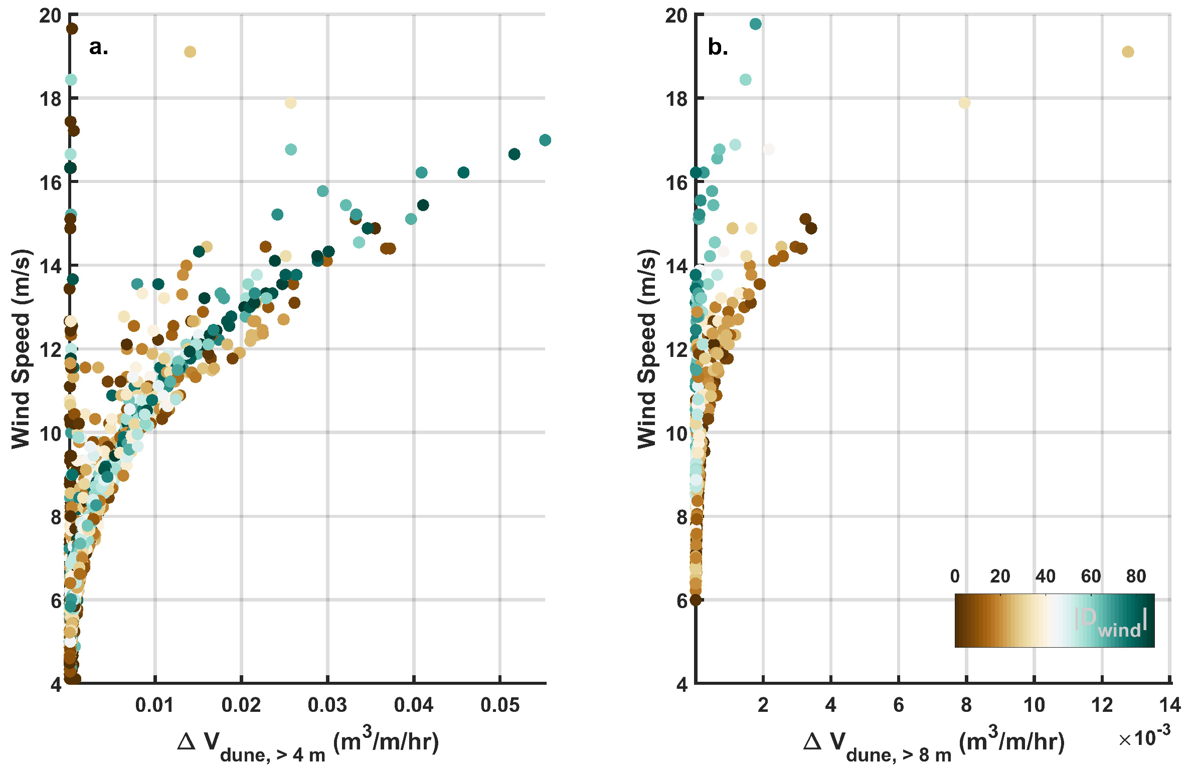
5.1.1. Aeolian Controls on Dune Growth

Although high wind velocities have the highest aeolian transport potential e.g., [38], many of the highest wind events co-occur with energetic waves and high SWLs (Figure 6). The combination of high H s and high SWL results in TWL in the collision regime numerous times per year at Oysterville. During periods when the TWL is near the dune toe, there is effectively no source area for aeolian transport – limiting aeolian contributions to dune growth under these forcing conditions. Dune growth instead occurs predominantly from aggregated transport under moderate wind conditions (6–12 m/s) (Figure 8d,i). Intermittent dune growth occurs throughout the year under these frequent moderate wind conditions (Figure 5c) which are above the threshold velocity for saltation (3–4 m/s based on the local grain size). The largest total aeolian-driven dune growth is simulated in the winter (Figure 5c and Figure 7b). This is consistent with observations of the timing of maximum dune growth at Oysterville, WA as noted by Cohn et al. [46]. The model results also agree with field observations that documented limited dune growth occurring during the summer period (Figure 5c and Figure 7b) when the beach is wide (high sediment supply) (Figure 5a,b) but wind velocities are typically low (Figure 6k).
The largest modeled source area for aeolian sediment transport is between the 3 and 4 m contours, although some sediment is sourced from lower elevations during lower tidal stages (Figure 7c). While this primary source region is located on the upper portion of the beach compartment (where the beach is defined between 1 m to 4 m), it coincides with the approximate mean model-predicted TWL elevation during the fall and winter seasons (not shown). Thus, this modeled region of active aeolian transport generally supports previous findings that the upper intertidal zone is an important source of sediment for dune growth e.g., [41].
Wind direction plays a role in controlling the apparent fetch length, which is thought to be an important factor for aeolian transport to dunes e.g., [35]. Windsurf simulations suggest that, in Oysterville, winds from the south and south-west provide the largest contribution to total dune growth (Figure 8e), in part because these are among the most common wind directions at the field site (Figure 8j). In Figure 9a, it is shown that the largest hourly dune growth rates in the simulation occur when the wind speeds are highest, mostly independent of the wind direction. That is, similar Δ V d u n e are simulated in the case of shore-normal or oblique winds for a given wind speed. There is some scatter in the hourly Δ V d u n e predictions (Figure 9a), reflecting in part the cosine effect e.g., [31] and/or unsaturated transport resulting from sediment supply limitations. However, when considering higher portions of the dune, shore-normal winds provide a larger contribution to dune growth for a given wind speed (Figure 9b). This is because, in the case of shore-normal winds, saltation can extend farther horizontally past the vegetation line because of a larger cross-shore component of the wind velocity and increased wind velocities on the dune face associated with flow acceleration over the steeper apparent dune slope.

5.1.2. Marine Controls on Dune Growth

While the paucity of observed dune erosion on some dissipative beaches has been hypothesized to be from synchronization of nearshore-beach-dune exchanges [26], which were thought to mask signs of erosion, modeled dune erosion at Oysterville, WA is infrequent because TWLs in the collision regime are not always erosional [51]. Windsurf predicts that numerous wave-driven events contribute to dune accretion at Oysterville during the 2016–2017 time frame (Figure 5, Figure 7, and Figure 8), with these events typically occurring during high SWL cases and/or during energetic wave periods (Figure 8). The simulations show that there were 3 h, all in October 2016, which resulted in at least 0.5 m 3 /m of marine-driven dune growth. Of note, these marine-contributions to dune growth are about an order of magnitude larger than the highest modeled hourly dune growth rates from aeolian sediment transport (Figure 9). Seven additional hours were simulated throughout fall and winter when marine-derived dune growth of at least 0.1 m 3 /m occurred. In Cohn et al. [46], it was estimated that up to ∼ 7 m 3 /m/year of dune growth at Oysterville, WA during the 2016–2017 period was driven by swash processes, similar in magnitude to the modeled 10.1 m 3 /m/year. It is important to note that the choice of the dune toe definition used for calculating volume changes has important implications for determining the relative contributions of marine and aeolian processes to dune growth. Traditional concavity-based metrics for defining the dune toe do not work well for low-gradient beach systems such as Oysterville. Therefore in Cohn et al. [46] and this study the dune toe is taken to be at 4 m based on local geomorphic and ecological characteristics. An alternative definition of the beach-dune interface would correspondingly alter the contributions of aeolian and marine processes to total foredune growth reported in this study. However, as this work demonstrates, the boundary between the beach and dune is not as simple as typically characterized in geomorphic studies.
While a positive Δ V d u n e is simulated most of the time when TWLs are in the collision regime, there are also some oceanographic conditions which instead produce wave-driven dune erosion (Figure 5c and Figure 8b,c). Therefore, the assertion that marine-related erosion can be masked by aeolian processes on dissipative coasts e.g., [26] is supported by the model under some conditions. This finding complicates attempts to decouple marine and aeolian contributions to dune sediment supply from field observations alone e.g., [46].

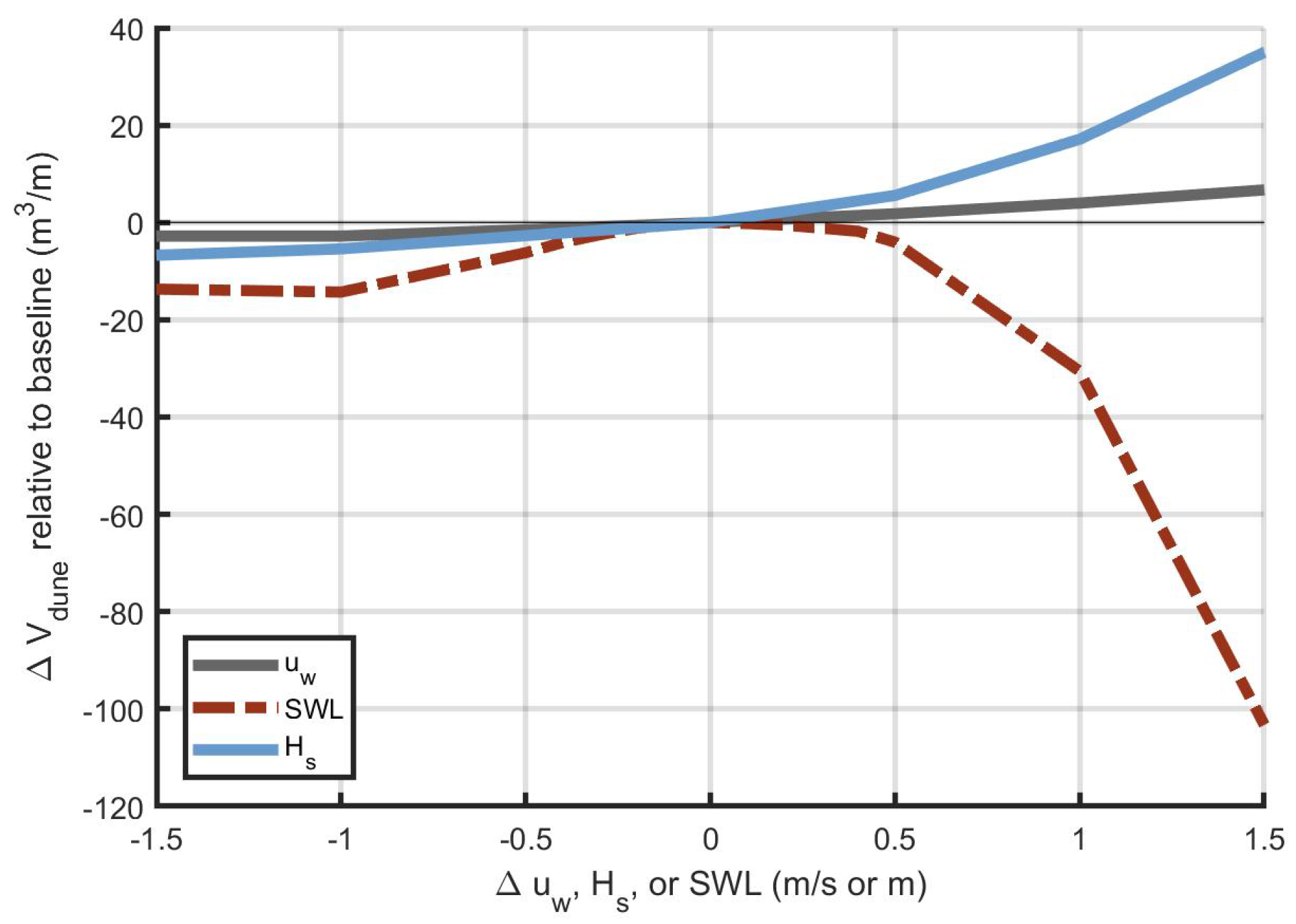
5.2. Sensitivity of Dune Growth to Environmental Perturbations

The ability to hindcast profile evolution at the field site provides some confidence that Windsurf is resolving the dominant morphodynamic processes at Oysterville. However, process-based models also provide the ability to explore environmental conditions outside of what was observed. Here additional simulations are completed to gain insight into the relative role of oceanographic and meteorological processes on dune evolution at the annual scale. To accomplish this, the year-long environmental time series of u w , SWL, and H s , were independently modified from the baseline (calibrated parameter) case, in which 17.7 m 3 /m of annual dune growth was simulated, to explore how the system would respond to environmental perturbations. First, these parameters are increased or decreased by fixed quantities. For example, one simulation was completed in which 0.5 m is added to every H s value input to the XBeach/Windsurf time series. While a fixed change in the SWL can be viewed as a proxy for mean sea level changes, there is no expectation for a uniform/constant increase in H s or u w even under climate change scenarios. However, these hypothetical exploratory simulations are devised to understand how these different environmental forcing factors may alter subsequent geomorphic evolution. Here constant additions or subtractions covering the range of −1.5 to 1.5 m (or m/s in the case of u w ), with increments of 0.5 m (m/s), were made to the environmental time series. Only one variable (either u w , SWL, or H s ) is altered in each simulation; all other attributes of the baseline case are maintained.
The results of this exercise are shown in Figure 10 and, as expected, indicate that decreasing wind speeds result in decreased volume gains to the dune and increasing wind speed drives increased Δ V d u n e . Because aeolian sediment transport scales to a third order power (Equation (2)) the relationship between u w and Δ V d u n e is nonlinear and therefore increases in wind speed (including higher values than those presented in Figure 10) result in an exponential type dune growth curve (not shown).
Increases in the SWL result in decreased dune growth relative to the baseline case (Figure 10) due to active wave breaking closer to the dune face and higher TWLs. The model simulates that even small increases in the SWL will actively destroy the dune ( Δ V d u n e relative to the baseline <−17.7 m 3 /m in Figure 10). However, decreases in the SWL also decrease the frequency that TWLs reach the dune toe, effectively cutting off any wave-induced sediment supply to the dune. Therefore, all cases with SWL that were lower than the hindcast time series had decreased Δ V d u n e relative to the baseline case. The observed SWL time series resulted in the largest dune growth of any simulated SWL cases.
Although increases in wave height are often associated with enhanced beach and dune erosion, the model simulations here suggest that increases in wave height may contribute positively to additional dune growth at Oysterville. This is consistent with model simulations in Cohn et al. [51] that found that as long as the dynamic still water level (DSWL), which is defined as the combination of the SWL and wave setup, falls below the dune toe that collisional wave impacts may contribute positively to growth of the lower portion of the dune at Oysterville. In this study, the exploratory Windsurf simulations suggest that uniform wave height increases of up to 1.5 m may encourage increased sediment delivery by marine processes to the base of the dune. However, it is expected that for more extreme wave height scenarios, increased frequency of the DSWL above the dune toe will instead promoted dune erosion. Assessing these extreme wave characteristic changes would require modifications to the Windsurf grid, which only extended to −9 m in this study, and therefore additional wave height simulations were not completed.

5.3. Windsurf Improvements and Future Applications

While Windsurf demonstrates the ability to simulate some realistic profile evolution in this application, the need for parameter calibration and the lack of a perfect match to data likely represents the effects of unknown physics, unincorporated physical processes, and/or oversimplified dynamics. Incorporating new processes or improving existing algorithms has the potential to increase the reliability and applicability of these tools in other settings. However, as both marine and aeolian sediment transport processes are highly complex, an improved physical understanding of coastal morphodynamic processes gained from field efforts is also essential to further improving these numerical capabilities e.g., [30]. Below some of the current key limitations of the Windsurf framework are highlighted.

5.3.1. Model Processes and Parameterizations

Of the three model cores in Windsurf, XBeach has the largest number of configurable parameters and is also generally the most sensitive to those model parameter choices. The fact that a separate high and low energy facAs and facSk were required for realistic model behavior implies that new formulations for these parameters that are more physically based may be necessary to make reliable forecasts of coastal progradation using XBeach in surfbeat mode. Recent improvements to XBeach add a non-hydrostatic correction term [98], which enables short waves to be modeled directly, and may provide a way forward. In non-hydrostatic mode, the nonlinearity of the wave shape is calculated directly, avoiding the need for facSk and facAs as these parameters are inherently included within the flow field. Therefore, using the wave resolving mode of XBeach could enable less site-specific model tuning. However, the non-hydrostatic model requires finer grid resolution which, for most applications, would substantially increase model run times. Furthermore, new sediment transport algorithms relevant for the non-hydrostatic model first need to be developed in the open-source code.
Although not explored in detail in this study, the algorithms parameterizing spatio-temporal vegetation density in CDM are currently simplified (a single, spatially uniform maximum ρ v e g is currently implemented). However, the vegetation plays a major role in the sand trapping capacity of sediment and resulting geomorphic shapes e.g., [21,99]. Sensitivity to dune grass parameters (e.g., height and density) were not explored in this study other than altering the m parameter during model calibration. As these ecological properties vary in both space and time and not all coastal systems are characterized by a single grass species, more robust approaches could be developed for use within the model. Therefore, while the currently implemented formulations may be suitable for understanding first order behavior, the addition of more robust ecological algorithms will provide added capability for simulating these dune growth behaviors for more applied cases e.g., [80].
There are additional moisture-related limiters to aeolian sediment transport in the coastal zone that were not assessed for this study. Much of the functionality to incorporate both groundwater and precipitation related effects are already coded into XBeach and Aeolis. Including these additional supply limiting factors may be important for some locations, particularly those characterized by high rainfall such as at Oysterville, WA.
On coastal systems characterized by storm-induced scarping and sharp topographic changes, the presently incorporated Weng et al. [81] solution for wind flow will have limitations in its applicability. For more complex settings a steady state wind solver may not be suitable. In these cases, a Navier-Stokes-based numerical solver could be implemented, as computational fluid dynamics methods have been shown to be successful at modeling complex flow patterns over a range of dune shapes e.g., [100,101]. The framework of Windsurf is modular by nature which allows for new models to be implemented and tested with relative ease.

5.3.2. External Sediment Supply

While the assumption of local mass conservation for the time scales investigated for this study are appropriate, when extending simulations to longer time frames incorporating external sediment supply inputs is imperative e.g., [5,102]. The definition of the offshore boundary in Windsurf currently allows for new sediment to be added to the local sediment budget via the replenishment of eroded near-boundary sediments. However, a more robust procedure for introducing both cross-shore shoreface feeding and longshore transport gradients would add value. A recent implementation of longshore gradients in transport into XBeach (lsgrad) provides one mechanism to do this for 1D applications based on an imposed length-scale for longshore transport gradients. Although not tested for this application, using this feature in Windsurf would require no changes to the model framework. Including these 1D imposed longshore transport gradients, or extending Windsurf to 2D area applications, would better represent coastal systems, including Oysterville, WA, where longshore transport gradients are important.

5.3.3. Computational Efficiency

The present Windsurf application is run in an offline approach through MATLAB. A python version of Windsurf is also in development which implements the basic model interface [103] and enables models to be run in an on-line approach, with boundary conditions updated on the fly. The latter approach significantly decreases model run times by eliminating computational overhead associated with frequent writing of model input and outputs to the disk. For the present application, completing one-year simulations takes approximately 2.5 days using 4 processors on a Dell C6100 Intel Xeon server running the CentOS 7 operating system. Reducing run times, even fractionally, may make simulating longer term (>years, decades) simulations more practical.

5.3.4. Further Testing of Framework Limitations

These first proof of concept Windsurf simulations at Oysterville, WA suggest that a coupled approach for assessing the co-evolution of the nearshore-beach-dune system provides value over independent modeling of discrete morphological units. As this is the first application of the modeling framework, the limits of Windsurf at simulating realistic behavior in other morphodynamic settings and for other environmental cases have not yet been demonstrated. Ideally, Windsurf is flexible enough to explore dune erosion, recovery, and growth across the continuum of reflective to dissipative beaches. However, to understand model limitations and extend model capabilities, the tool needs to first be applied in other data rich settings. Similarly, additional future work should aim to characterize model sensitivity to input choices, particularly for spatially variable properties such as sediment grain size and ecological properties.

6. Conclusions

A new coupled numerical modeling framework, Windsurf, can simulate the co-evolution of the nearshore, beach, and dunes. Consistent with detailed morphologic measurements at a progradational field site, the model successfully simulates seasonal cycles of beach growth in summer, shoreline recession in winter, and net dune growth annually. The modeling results are also consistent with findings from field observations, both of which suggest that both marine and aeolian processes directly contribute to the growth of coastal foredunes on this high energy, dissipative coastline. The importance of, and challenges involved in, distinguishing between marine and aeolian controls on dune evolution revealed by field observations and model simulations highlight the need for further exploration and development of coupled tools bridging the land-sea interface for coastal landscape evolution. While significant efforts are required to further test the capabilities and limitations of Windsurf and its model cores, the Windsurf framework provides a new platform to explore complex interactions between the subaqueous and subaerial zones of the coastal profile for a variety of exploratory and applied applications.

Supplementary Materials

The matlab version of the Windsurf code used in this study can be freely accessed at https://github.com/ncohn/Windsurf.

Author Contributions

All the co-authors contributed to the initial development of the Windsurf framework. N.C., B.M.H., and E.B.G. wrote the Windsurf code and contributed to model core improvements needed to implement Windsurf. N.C., S.d.V. and P.R. collected the field data. N.C. performed the field data analysis and completed the Windsurf model application at the Oysterville field site. N.C. and P.R. wrote the manuscript. The remaining co-authors contributed to editing and improvement of this paper.

Funding

This research was supported by the Geomorphology and Land Use Dynamics Program at the U.S. National Science Foundation (NSF) under grant EAR-1561847 for field data collection and model application at Oysterville, WA. Field data collection at Oysterville was also funded in part by the Northwest Association of Networked Ocean Observing System (NANOOS) and the U.S. Army Corps of Engineers Portland District. General Windsurf model development was supported by the U.S. National Oceanic and Atmospheric Administration (NOAA) through the Ecological Effects of Sea Level Rise grant NA15NOS4780172 and via two American Shore and Beach Preservation Association Technology Challenge grants (one to OSU and one to UNC-CH), as well as funding from the Long-term Ecological Research Program at NSF under grant DEB-123773 via a subaward to UNC-CH from the University of Virginia. The APC was funded by NSF grant funds.

Acknowledgments

We thank the many researchers at Oregon State University and the Washington Department of Ecology who contributed to field efforts during SEDEX 2 . Additional thanks are given to Guy Gelfenbaum (USGS) and Eugene Bodrero (Dyacon, Inc.) for loaning equipment for SEDEX 2 used for model forcing in this study. We also thank Dano Roelvink (Deltares/UNESCO) for participating in many conversations about XBeach and numerical model coupling which were instrumental in the development of Windsurf.

Conflicts of Interest

The authors declare no conflict of interest.

References

  1. Cowell, P.; Thom, B.G. Morphodynamics of coastal evolution. In Coastal Evolution; Carter, R.W.G., Woodroffe, C.D., Eds.; Cambridge University Press: New York, NY, USA, 1995; pp. 33–86. [Google Scholar]
  2. Short, A.; Hesp, P. Wave, beach and dune interactions in southeastern Australia. Mar. Geol. 1982, 48, 259–284. [Google Scholar] [CrossRef]
  3. Komar, P. Beach Processes and Sedimentation; Prentice Hall: Upper Saddle River, NJ, USA, 1998. [Google Scholar]
  4. Wright, L.; Thom, B. Coastal depositional landforms. Prog. Phys. Geogr. Earth Environ. 1977, 1, 412–459. [Google Scholar] [CrossRef]
  5. Cowell, P.; Stive, M.; Niedoroda, A.; de Vriend, H.; Swift, D.; Kaminsky, G.; Capobianco, M. The coastal-tract (part 1): A conceptual approach to aggregated modeling of low-order coastal change. J. Coast. Res. 2003, 812–827. [Google Scholar]
  6. Gallop, S.L.; Collins, M.; Pattiaratchi, C.B.; Eliot, M.J.; Bosserelle, C.; Ghisalberti, M.; Collins, L.B.; Eliot, I.; Erftemeijer, P.L.A.; Larcombe, P.; et al. Challenges in transferring knowledge between scales in coastal sediment dynamics. Front. Mar. Sci. 2015, 2. [Google Scholar] [CrossRef]
  7. Ruggiero, P.; Kaminsky, G.M.; Gelfenbaum, G.; Cohn, N. Morphodynamics of prograding beaches: A synthesis of seasonal- to century-scale observations of the Columbia River littoral cell. Mar. Geol. 2016, 376, 51–68. [Google Scholar] [CrossRef] [Green Version]
  8. Sherman, D.J.; Bauer, B.O. Dynamics of beach-dune systems. Prog. Phys. Geogr. 1993, 17, 413–447. [Google Scholar] [CrossRef]
  9. Sallenger, A. Storm impact scale for barrier islands. J. Coast. Res. 2000, 16, 890–895. [Google Scholar]
  10. Elko, N.; Brodie, K.; Stockdon, H.; Nordstrom, K.; Houser, C.; McKenna, K.; Moore, L.; Rosati, J.; Ruggiero, R.; Thuman, R.; et al. Dune management challenges on developed coasts. Shore Beach 2016, 84, 15–28. [Google Scholar]
  11. Walker, I.J.; Davidson-Arnott, R.G.; Bauer, B.O.; Hesp, P.A.; Delgado-Fernandez, I.; Ollerhead, J.; Smyth, T.A. Scale-dependent perspectives on the geomorphology and evolution of beach-dune systems. Earth-Sci. Rev. 2017, 171, 220–253. [Google Scholar] [CrossRef]
  12. Arkema, K.K.; Guannel, G.; Verutes, G.; Wood, S.A.; Guerry, A.; Ruckelshaus, M.; Kareiva, P.; Lacayo, M.; Silver, J.M. Coastal habitats shield people and property from sea-level rise and storms. Nat. Clim. Chang. 2013, 3, 913–918. [Google Scholar] [CrossRef]
  13. Martínez, M.; Psuty, N. Coastal Dunes; Springer: Berlin, Germany, 2004. [Google Scholar]
  14. Miller, T.E.; Gornish, E.S.; Buckley, H.L. Climate and coastal dune vegetation: disturbance, recovery, and succession. Plant Ecol. 2010, 206, 97–104. [Google Scholar] [CrossRef]
  15. Sutton-Grier, A.E.; Wowk, K.; Bamford, H. Future of our coasts: The potential for natural and hybrid infrastructure to enhance the resilience of our coastal communities, economies and ecosystems. Environ. Sci. Policy 2015, 51, 137–148. [Google Scholar] [CrossRef] [Green Version]
  16. Psuty, N. The coastal foredune: A morphological basis for regional coastal dune development. In Coastal Dunes; Martínez, M., Psuty, N., Eds.; Springer: Berlin, Germany, 2004; pp. 11–27. [Google Scholar]
  17. Hesp, P.A. Conceptual models of the evolution of transgressive dune field systems. Geomorphology 2013, 199, 138–149. [Google Scholar] [CrossRef]
  18. Zinnert, J.C.; Stallins, J.A.; Brantley, S.T.; Young, D.R. Crossing Scales: The Complexity of Barrier-Island Processes for Predicting Future Change. BioScience 2016, 67, 39–52. [Google Scholar] [CrossRef]
  19. Luna, M.C.; Parteli, E.J.; Durán, O.; Herrmann, H.J. Model for the genesis of coastal dune fields with vegetation. Geomorphology 2011, 129, 215–224. [Google Scholar] [CrossRef]
  20. Van Dijk, P.M.; Arens, S.M.; van Boxel, J.H. Aeolian processes across transverse dunes. II: modelling the sediment transport and profile development. Earth Surf. Process. Landf. 1999, 24, 319–333. [Google Scholar] [CrossRef] [Green Version]
  21. Zarnetske, P.L.; Hacker, S.D.; Seabloom, E.W.; Ruggiero, P.; Killian, J.R.; Maddux, T.B.; Cox, D. Biophysical feedback mediates effects of invasive grasses on coastal dune shape. Ecology 2012, 93, 1439–1450. [Google Scholar] [CrossRef] [PubMed]
  22. Durán, O.; Moore, L.J. Vegetation controls on the maximum size of coastal dunes. Proc. Natl. Acad. Sci. USA 2013, 110, 17217–17222. [Google Scholar] [CrossRef] [PubMed] [Green Version]
  23. Keijsers, J.; Groot, A.D.; Riksen, M. Vegetation and sedimentation on coastal foredunes. Geomorphology 2015, 228, 723–734. [Google Scholar] [CrossRef]
  24. Davidson-Arnott, R.; Law, M. Measurement and prediction of long-term sediment supply to coastal foredunes. J. Coast. Res. 1996, 654–663. [Google Scholar]
  25. De Vries, S.; Southgate, H.; Kanning, W.; Ranasinghe, R. Dune behavior and aeolian transport on decadal timescales. Coastal Engineering 2012, 67, 41–53. [Google Scholar] [CrossRef]
  26. Houser, C. Synchronization of transport and supply in beach-dune interaction. Prog. Phys. Geogr. 2009, 33, 733–746. [Google Scholar] [CrossRef]
  27. Ollerhead, J.; Davidson-Arnott, R.; Walker, I.J.; Mathew, S. Annual to decadal morphodynamics of the foredune system at Greenwich Dunes, Prince Edward Island, Canada. Earth Surf. Process. Landf. 2012, 38, 284–298. [Google Scholar] [CrossRef]
  28. Davidson-Arnott, R.G.; MacQuarrie, K.; Aagaard, T. The effect of wind gusts, moisture content and fetch length on sand transport on a beach. Geomorphology 2005, 68, 115–129. [Google Scholar] [CrossRef]
  29. Nickling, W.G.; Ecclestone, M. The effects of soluble salts on the threshold shear velocity of fine sand. Sedimentology 1981, 28, 505–510. [Google Scholar] [CrossRef]
  30. Brakenhoff, L.; Smit, Y.; Donker, J.; Ruessink, G. Tide-induced variability in beach surface moisture: Observations and modelling. Earth Surf. Process. Landf. 2018. [Google Scholar] [CrossRef]
  31. Bauer, B.O.; Davidson-Arnott, R.G. A general framework for modeling sediment supply to coastal dunes including wind angle, beach geometry, and fetch effects. Geomorphology 2003, 49, 89–108. [Google Scholar] [CrossRef]
  32. Delgado-Fernandez, I. A review of the application of the fetch effect to modelling sand supply to coastal foredunes. Aeolian Res. 2010, 2, 61–70. [Google Scholar] [CrossRef] [Green Version]
  33. Hoonhout, B.M.; de Vries, S. A process-based model for aeolian sediment transport and spatiotemporal varying sediment availability. J. Geophys. Res. Earth Surf. 2016, 121, 1555–1575. [Google Scholar] [CrossRef] [Green Version]
  34. Bauer, B.; Davidson-Arnott, R.; Hesp, P.; Namikas, S.; Ollerhead, J.; Walker, I. Aeolian sediment transport on a beach: Surface moisture, wind fetch, and mean transport. Geomorphology 2009, 105, 106–116. [Google Scholar] [CrossRef]
  35. Davidson-Arnott, R.; Hesp, P.; Ollerhead, J.; Walker, I.; Bauer, B.; Delgado-Fernandez, I.; Smyth, T. Sediment Budget Controls on Foredune Height: Comparing Simulation Model Results with Field Data. Earth Surf. Process. Landf. 2018. [Google Scholar] [CrossRef]
  36. Jackson, D.W.T.; Cooper, A. Beach fetch distance and aeolian sediment transport. Sedimentology 1999, 46, 517–522. [Google Scholar] [CrossRef]
  37. Bascom, W.N. The relationship between sand size and beach-face slope. Trans. Am. Geophys. Union 1951, 32, 866. [Google Scholar] [CrossRef]
  38. Bagnold, R.A. The Transport of Sand by Wind. Geogr. J. 1937, 89, 409. [Google Scholar] [CrossRef]
  39. Carter, R.; Rihan, C. Shell and pebble pavements on beaches: Examples from the north coast of Ireland. CATENA 1978, 5, 365–374. [Google Scholar] [CrossRef]
  40. Neuman, C.M.; Li, B.; Nash, D. Micro-topographic analysis of shell pavements formed by aeolian transport in a wind tunnel simulation. J. Geophys. Res. Earth Surf. 2012, 117. [Google Scholar] [CrossRef] [Green Version]
  41. De Vries, S.; Arens, S.; de Schipper, M.; Ranasinghe, R. Aeolian sediment transport on a beach with a varying sediment supply. Aeolian Res. 2014, 15, 235–244. [Google Scholar] [CrossRef]
  42. De Vries, S.; Verheijen, A.; Hoonhout, B.; Vos, S.; Cohn, N.; Ruggiero, P. Measured spatial variability of beach erosion due to aeolian processes. In Proceedings of the Coastal Dynamics Conference 2017, Helsingør, Denmark, 12–16 June 2017. [Google Scholar]
  43. Hoonhout, B.; de Vries, S. Aeolian sediment supply at a mega nourishment. Coast. Eng. 2017, 123, 11–20. [Google Scholar] [CrossRef]
  44. Hoonhout, B.; de Vries, S. Field measurements on spatial variations in aeolian sediment availability at the Sand Motor mega nourishment. Aeolian Res. 2017, 24, 93–104. [Google Scholar] [CrossRef]
  45. Aagaard, T.; Davidson-Arnott, R.; Greenwood, B.; Nielsen, J. Sediment supply from shoreface to dunes: linking sediment transport measurements and long-term morphological evolution. Geomorphology 2004, 60, 205–224. [Google Scholar] [CrossRef]
  46. Cohn, N.; Ruggiero, P.; de Vries, S.; Kaminsky, G. New insights on the relative contributions of marine and aeolian processes to coastal foredune growth. Geophys. Res. Lett. 2018, 45, 4965–4973. [Google Scholar] [CrossRef]
  47. Stockdon, H.F.; Sallenger, A.H.; Holman, R.A.; Howd, P.A. A simple model for the spatially-variable coastal response to hurricanes. Mar. Geol. 2007, 238, 1–20. [Google Scholar] [CrossRef]
  48. Splinter, K.D.; Kearney, E.T.; Turner, I.L. Drivers of alongshore variable dune erosion during a storm event: Observations and modelling. Coast. Eng. 2018, 131, 31–41. [Google Scholar] [CrossRef]
  49. Saye, S.; van der Wal, D.; Pye, K.; Blott, S. Beach–dune morphological relationships and erosion/accretion: An investigation at five sites in England and Wales using LIDAR data. Geomorphology 2005, 72, 128–155. [Google Scholar] [CrossRef]
  50. Burroughs, S.M.; Tebbens, S.F. Dune Retreat and Shoreline Change on the Outer Banks of North Carolina. J. Coast. Res. 2008, 2, 104–112. [Google Scholar] [CrossRef]
  51. Cohn, N.; Ruggiero, P.; García-Medina, G.; Anderson, D.; Serafin, K.; Biel, R. Environmental and morphologic control on wave induced dune response. Geomorphology. in press. [CrossRef]
  52. Roelvink, D.; Reniers, A.; van Dongeren, A.; van Thiel de Vries, J.; McCall, R.; Lescinski, J. Modelling storm impacts on beaches, dunes and barrier islands. Coast. Eng. 2009, 56, 1133–1152. [Google Scholar] [CrossRef]
  53. Pender, D.; Karunarathna, H. A statistical-process based approach for modelling beach profile variability. Coast. Eng. 2013, 81, 19–29. [Google Scholar] [CrossRef] [Green Version]
  54. Stockdon, H.; Thompson, D.; Plant, N.; Long, J. Evaluation of wave runup predictions from numerical and parametric models. Coast. Eng. 2014, 92, 1–11. [Google Scholar] [CrossRef]
  55. De Winter, R.; Gongriep, F.; Ruessink, B. Observations and modeling of alongshore variability in dune erosion at Egmond aan Zee, the Netherlands. Coast. Eng. 2015, 99, 167–175. [Google Scholar] [CrossRef]
  56. McCall, R.; Van Thiel de Vries, J.; Plant, N.; Dongeren, A.V.; Roelvink, J.; Thompson, D.; Reniers, A. Two-dimensional time dependent hurricane overwash and erosion modeling at Santa Rosa Island. Coast. Eng. 2010, 57, 668–683. [Google Scholar] [CrossRef]
  57. Van Dongeren, A.; Bolle, A.; Vousdoukas, M.I.; Plomaritis, T.; Eftimova, P.; Williams, J.; Armaroli, C.; Idier, D.; Geer, P.V.; Van Thiel de Vries, J.; et al. MICORE: Dune erosion and overwash model validation with data from nine European field sites. In Proceedings of the Coastal Dynamics Conference, Tokyo, Japan, 7–11 September 2009; Mizuguchi, M., Sato, S., Eds.; World Scientific: Tokyo, Japan, 2009. [Google Scholar] [CrossRef]
  58. Buckley, M.; Lowe, R.; Hansen, J. Evaluation of nearshore wave models in steep reef environments. Ocean Dyn. 2014, 64, 847–862. [Google Scholar] [CrossRef]
  59. Roelvink, D.; McCall, R.; Mehvar, S.; Nederhoff, K.; Dastgheib, A. Improving predictions of swash dynamics in XBeach: The role of groupiness and incident-band runup. Coast. Eng. 2018, 134, 103–123. [Google Scholar] [CrossRef]
  60. Harley, M.; Armaroli, C.; Ciavola, P. Evaluation of XBeach predictions for a real-time warning system in Emilia-Romagna, Northern Italy. J. Coast. Res. 2011, 64, 1861–1863. [Google Scholar]
  61. Splinter, K.D.; Palmsten, M.L. Modeling dune response to an East Coast Low. Mar. Geol. 2012, 329–331, 46–57. [Google Scholar] [CrossRef]
  62. Splinter, K.D.; Carley, J.T.; Golshani, A.; Tomlinson, R. A relationship to describe the cumulative impact of storm clusters on beach erosion. Coast. Eng. 2014, 83, 49–55. [Google Scholar] [CrossRef]
  63. Verheyen, B.; Gruwez, V.; Zimmermann, N.; Wauters, P.; Bolle, A. Medium term time-dependent morphodynamic modelling of beach profile evolution in Ada, Ghana. In Proceedings of the 11th International Conference on Hydroscience and Engineering, Hamburg, Germany, 28 September–2 October 2014; Lehfeldt, R., Kopmann, R., Eds.; Bundesanstalt fuer Wasserbau: Karlsruhe, Germany, 2014. [Google Scholar]
  64. Ramakrishnan, R.; Agrawal, R.; Remya, P.; NagaKumar, K.; Demudu, G.; Rajawat, A.; Nair, B.; Rao, K.N. Modelling coastal erosion: A case study of Yarada beach near Visakhapatnam, east coast of India. Ocean Coast. Manag. 2018, 156, 239–248. [Google Scholar] [CrossRef]
  65. Roelvink, D.; van Dongeren, A.; McCall, R.; Hoonhout, B.; van Rooijen, A.; van Geer, P.; de Vet, L.; Nederhoff, K.; Quataert, E. XBeach Technical Reference: Kingsday Release; Technical report; Deltares: Delft, The Netherlands, 2015. [Google Scholar]
  66. Holthuijsen, L.; Booij, N.; Herbers, T. A prediction model for stationary, short-crested waves in shallow water with ambient currents. Coast. Eng. 1989, 13, 23–54. [Google Scholar] [CrossRef]
  67. Galappatti, G.; Vreugdenhil, C.B. A depth-integrated model for suspended sediment transport. J. Hydraul. Res. 1985, 23, 359–377. [Google Scholar] [CrossRef]
  68. Vousdoukas, M.I.; Ferreira, Ó.; Almeida, L.P.; Pacheco, A. Toward reliable storm-hazard forecasts: XBeach calibration and its potential application in an operational early-warning system. Ocean Dyn. 2012, 62, 1001–1015. [Google Scholar] [CrossRef]
  69. Simmons, J.A.; Harley, M.D.; Marshall, L.A.; Turner, I.L.; Splinter, K.D.; Cox, R.J. Calibrating and assessing uncertainty in coastal numerical models. Coast. Eng. 2017, 125, 28–41. [Google Scholar] [CrossRef]
  70. Dissanayake, P.; Brown, J.; Karunarathna, H. Impacts of storm chronology on the morphological changes of the Formby beach and dune system, UK. Nat. Hazards Earth Syst. Sci. 2015, 15, 1533–1543. [Google Scholar] [CrossRef] [Green Version]
  71. van Rhee, C. Sediment Entrainment at High Flow Velocity. J. Hydraul. Eng. 2010, 136, 572–582. [Google Scholar] [CrossRef]
  72. Reniers, A.J.H.M. Morphodynamic modeling of an embayed beach under wave group forcing. J. Geophys. Res. 2004, 109. [Google Scholar] [CrossRef] [Green Version]
  73. Reyns, J.; Dastgheib, A.; Ranasinghe, R.; Luijendijk, A.; Walstra, D.J.; Roelvink, D. Morphodynamic upscaling with the morfac approach in tidal conditions: the critical morfac. In Proceedings of the Coastal Engineering Conference, Seoul, Korea, 15–20 June 2014; Lynett, P., Ed.; Coastal Engineering Research Council: Seoul, Korea, 2014; p. 27. [Google Scholar] [CrossRef]
  74. Sauermann, G.; Kroy, K.; Herrmann, H.J. Continuum saltation model for sand dunes. Phys. Rev. E 2001, 64. [Google Scholar] [CrossRef] [PubMed]
  75. Durán, O.; Herrmann, H.J. Vegetation Against Dune Mobility. Phys. Rev. Lett. 2006, 97. [Google Scholar] [CrossRef]
  76. Parteli, E.J.R.; Durán, O.; Tsoar, H.; Schwämmle, V.; Herrmann, H.J. Dune formation under bimodal winds. Proc. Natl. Acad. Sci. USA 2009, 106, 22085–22089. [Google Scholar] [CrossRef] [Green Version]
  77. Schwämmle, V.; Herrmann, H.J. A model of Barchan dunes including lateral shear stress. Eur. Phys. J. E 2005, 16, 57–65. [Google Scholar] [CrossRef] [Green Version]
  78. Moore, L.J.; Vinent, O.D.; Ruggiero, P. Vegetation control allows autocyclic formation of multiple dunes on prograding coasts. Geology 2016, 44, 559–562. [Google Scholar] [CrossRef] [Green Version]
  79. Durán, O.; Moore, L.J. Barrier island bistability induced by biophysical interactions. Nat. Clim. Chang. 2015, 5, 158–162. [Google Scholar] [CrossRef]
  80. Goldstein, E.B.; Moore, L.J.; Vinent, O.D. Lateral vegetation growth rates exert control on coastal foredune hummockiness and coalescing time. Earth Surf. Dyn. 2017, 5, 417–427. [Google Scholar] [CrossRef] [Green Version]
  81. Weng, W.S.; Hunt, J.C.R.; Carruthers, D.J.; Warren, A.; Wiggs, G.F.S.; Livingstone, I.; Castro, I. Air flow and sand transport over sand-dunes. In Aeolian Grain Transport; Springer: Vienna, Austria, 1991; pp. 1–22. [Google Scholar]
  82. Hunt, J.C.R.; Leibovich, S.; Richards, K.J. Turbulent shear flows over low hills. Q. J. R. Meteorol. Soc. 1988, 114, 1435–1470. [Google Scholar] [CrossRef]
  83. Raupach, M.R.; Gillette, D.A.; Leys, J.F. The effect of roughness elements on wind erosion threshold. J. Geophys. Res. Atmos. 1993, 98, 3023–3029. [Google Scholar] [CrossRef]
  84. De Vries, S.; van Thiel de Vries, J.; van Rijn, L.; Arens, S.; Ranasinghe, R. Aeolian sediment transport in supply limited situations. Aeolian Res. 2014, 12, 75–85. [Google Scholar] [CrossRef]
  85. Belly, P. Sand Movement by Wind; Technical Report CERC Memorandum 1; U.S. Army Corps of Engineers: Vicksburg, MS, USA, 1964.
  86. Ruggiero, P.; Kaminsky, G.M.; Gelfenbaum, G.; Voigt, B. Seasonal to Interannual Morphodynamics along a High-Energy Dissipative Littoral Cell. J. Coast. Res. 2005, 213, 553–578. [Google Scholar] [CrossRef]
  87. Barnard, P.L.; Hoover, D.; Hubbard, D.M.; Snyder, A.; Ludka, B.C.; Allan, J.; Kaminsky, G.M.; Ruggiero, P.; Gallien, T.W.; Gabel, L.; et al. Extreme oceanographic forcing and coastal response due to the 2015–2016 El Niño. Nat. Commun. 2017, 8, 14365. [Google Scholar] [CrossRef] [Green Version]
  88. Cohn, N.; Ruggiero, P.; de Vries, S.; García-Medina, G. Beach growth driven by intertidal sandbar welding. In Proceedings of the Coastal Dynamics Conference, Helsingør, Denmark, 12–16 June 2017; pp. 1059–1069. [Google Scholar]
  89. Cohn, N.; Ruggiero, P. The influence of seasonal to interannual nearshore profile variability on extreme water levels: Modeling wave runup on dissipative beaches. Coast. Eng. 2016, 115, 79–92. [Google Scholar] [CrossRef]
  90. Gelfenbaum, G.; Stevens, A.W.; Miller, I.; Warrick, J.A.; Ogston, A.S.; Eidam, E. Large-scale dam removal on the Elwha River, Washington, USA: Coastal geomorphic change. Geomorphology 2015, 246, 649–668. [Google Scholar] [CrossRef] [Green Version]
  91. Hapke, C.; Himmelstoss, E.; Kratzmann, M.; List, J.; Thieler, E. National Assessment of Shoreline Change: Historical Shoreline Change along the New England and Mid-Atlantic Coasts; Technical Report Open-File Report 2010-1118; U.S. Geological Survey: Reston, VA, USA, 2011.
  92. Booij, N.; Ris, R.C.; Holthuijsen, L.H. A third-generation wave model for coastal regions: 1. Model description and validation. J. Geophys. Res. Oceans 1999, 104, 7649–7666. [Google Scholar] [CrossRef] [Green Version]
  93. Carignan, K.; Taylor, L.; Eakins, B.; Warnken, R. Digital Elevation Model of Astoria, Oregon: Procedures, Data Sources and Analysis; Technical Report NESDIS NGDC-22; U.S. National Oceanic and Atmospheric Administration, U.S. Dept. of Commerce: Boulder, CO, USA, 2009.
  94. Allan, J.; Ruggiero, P.; Cohn, N.; García-Medina, G.; Brien, F.O.; Serafin, K.; Stimley, L.; Roberts, J. Coastal Flood Hazard Study, Lincoln County, Oregon; Technical Report O-15-06; Oregon Department of Geology and Mineral Industries: Newport, OR, USA, 2015.
  95. Berard, N.A.; Mulligan, R.P.; da Silva, A.M.F.; Dibajnia, M. Evaluation of XBeach performance for the erosion of a laboratory sand dune. Coast. Eng. 2017, 125, 70–80. [Google Scholar] [CrossRef]
  96. Oreskes, N.; Belitz, K. Philosophical issues in model assessment. In Model Validation: Perspectives in hydrological science; Anderson, M., Bates, P., Eds.; John Wiley and Sons: Hoboken, NJ, USA, 2001; pp. 23–41. [Google Scholar]
  97. Thieler, E.; Pilkey, H.; Young, R.; Bush, D.; Chai, F. The use of mathematical models to predict beach behavior for US coastal engineering: A critical review. J. Coast. Res. 2000, 48–70. [Google Scholar]
  98. McCall, R.; Masselink, G.; Poate, T.; Roelvink, J.; Almeida, L. Modelling the morphodynamics of gravel beaches during storms with XBeach-G. Coast. Eng. 2015, 103, 52–66. [Google Scholar] [CrossRef] [Green Version]
  99. Hacker, S.D.; Zarnetske, P.; Seabloom, E.; Ruggiero, P.; Mull, J.; Gerrity, S.; Jones, C. Subtle differences in two non-native congeneric beach grasses significantly affect their colonization, spread, and impact. Oikos 2012, 121, 138–148. [Google Scholar] [CrossRef]
  100. Smyth, T.A.; Jackson, D.W.; Cooper, J.A.G. High resolution measured and modelled three-dimensional airflow over a coastal bowl blowout. Geomorphology 2012, 177–178, 62–73. [Google Scholar] [CrossRef]
  101. Smyth, T.A.; Hesp, P.A. Aeolian dynamics of beach scraped ridge and dyke structures. Coast. Eng. 2015, 99, 38–45. [Google Scholar] [CrossRef] [Green Version]
  102. Anthony, E.J. Beach-ridge development and sediment supply: examples from West Africa. Mar. Geol. 1995, 129, 175–186. [Google Scholar] [CrossRef]
  103. Peckham, S.D.; Hutton, E.W.; Norris, B. A component-based approach to integrated modeling in the geosciences: The design of CSDMS. Comput. Geosci. 2013, 53, 3–12. [Google Scholar] [CrossRef]
Figure 1. Cross-shore schematic of the coupled Windsurf modeling framework showing the general processes resolved by the model cores.
Jmse 07 00013 g001
Figure 2. Schematic representing the general Windsurf model framework which includes three standalone numerical models (XBeach, CDM, Aeolis) that are coupled offline through a back-end MATLAB interface. Major processes resolved within each model core and the outputs exchanged by the coupler are shown. Black arrows show the order of model processes and model core boundary condition exchanges. Morphology and total water level information is also exchanged between XBeach and Aeolis, as denoted by the dotted grey arrow.
Jmse 07 00013 g002
Figure 3. (a) Map of the Oysterville field site on the Long Beach Peninsula, WA, USA. The locations of nearby wave (Coastal Data Information Program (CDIP) 036), tide (Toke Point, WA), and wind measurements (Toke Point, WA) and the Simulating Waves Nearshore (SWAN) wave model domain used to transform offshore waves locally to Oysterville are also shown. (b,c) Aerial photos of nearshore, beach, and dune at Oysterville, WA taken on 9 August 2016 during low energy wave conditions (H s ∼ 1.5 m). Photo (c) is taken from directly above the foredune crest where a camera mast system (shown) and meteorological station (not shown) were located during SEDEX 2 .
Jmse 07 00013 g003
Figure 4. Measurements of coastal profile change of the nearshore, beach, and dune over a 1-year period between August 2016 (grey line) to August 2017 (black line). The calibrated Windsurf model prediction after one year is shown in yellow.
Jmse 07 00013 g004
Figure 5. Measured (grey lines) versus calibrated model simulations (yellow lines) of (a) MHW shoreline change, (b) beach volume change, and (c) dune volume change. Error bars are added for the volumetric measurements assuming a ± 0.08 m vertical error for the topographic measurements.
Jmse 07 00013 g005
Figure 6. Locally measured (red) and transformed (grey) still water levels (a), significant wave heights (b), peak wave periods (c), wave direction (d), wind speed (e), and wind direction (f) for a 1 month period in summer 2016. The continuous, year-long time series of environmental parameters between summer 2016 and summer 2017, which includes the one-month period (shaded), for input to Windsurf is shown in panels (gl) using the transformed variables, where applicable. Please note that, as per model core conventions, 270 is shore-normal for D w a v e (nautical convention) and 0 is shore-normal (onshore directed) for D w i n d .
Jmse 07 00013 g006
Figure 7. (a) Comparison of volume changes (binned vertically in 0.5 m increments) between the field measurements (dashed grey line) and model predictions (dashed yellow line) at annual scale for the calibrated simulation. (b) Windsurf output with vertically binned volume changes broken down by the seasonal cycles of deposition. (c) Windsurf simulated volume changes are distinguished between marine (solid blue line) and aeolian (solid orange line) contributions. Please note that the x-axis limits change on each panel.
Jmse 07 00013 g007
Figure 8. Marine (blue line) and aeolian (orange line) contributions to dune volume change binned based on (a) SWL, (b) H s , (c) T p , (d) u, and (e) D w i n d for the one-year calibrated Windsurf simulation. The frequency of occurrence of each (f) SWL, (g) H s , (h) T p , (i) u, and (j) D w i n d forcing condition are also shown for the one-year record for comparison.
Jmse 07 00013 g008
Figure 9. Hourly Windsurf simulated Δ V d u n e above the 4 m contour (a) and 8 m contour (b) resulting from aeolian processes (marine-related Δ V d u n e are excluded) plotted against wind speed. Colors represent the absolute value of wind direction relative to shore-normal.
Jmse 07 00013 g009
Figure 10. Sensitivity of Δ V d u n e to uniform changes to the environmental time series of u w (light blue), SWL (dotted red), and H s (grey). Positive numbers indicate that more dune growth was predicted relative to the baseline (calibrated) model simulation of 17.7 m 3 /m.
Jmse 07 00013 g010
Table 1. Root mean squared error (RMSE) and bias ( Δ μ ) of transformed oceanographic and meteorological measurements, used to drive Windsurf boundary conditions, compared to local measurements. The local marine measurements used for comparison are 42 days and are 291 days for the wind measurements.
Environmental ParameterLocal Measurement Transformed DatasetLocallyRMSE Δ μ
SWLAWACToke Point0.29 m0.04 m
H s CDIP 462110.12 m<0.01 m
T p 1.7 s0.03 s
D w a v e 8 ° 0.3 °
uDyaconToke Point1.13 m/s−0.37 m/s
D w i n d 25.5 0.2
Table 2. Listing of range of values tested and optimum parameter settings based on the calibration routine.
Model ParameterMode CoreMin Value TestedMax Value TestCalibrated Value
mCDM0.0050.200.104
CbAeolis0.201.500.370
facSk(low energy)XBeach0.100.500.123
facSk(high energy)0.000.150.057
facAs(low energy)0.100.500.273
facAs(high energy)0.000.150.044

