Numerical Analysis of Influence of the Hull Couple Motion on the Propeller Exciting Force Characteristics

1
China Ship Scientific Research Center, Wuxi 214082, China
2
Jiangsu Key Laboratory of Green Ship Technology, Wuxi 214082, China
3
College of Shipbuilding Engineering, Harbin Engineering University, Harbin 150001, China
*
Author to whom correspondence should be addressed.
J. Mar. Sci. Eng. 2019, 7(10), 330; https://doi.org/10.3390/jmse7100330
Submission received: 31 August 2019
/
Revised: 17 September 2019
/
Accepted: 19 September 2019
/
Published: 23 September 2019
(This article belongs to the Special Issue Selected Papers from the Sixth International Symposium on Marine Propulsors)
Abstract
:The numerical calculation was performed for the KRISO Container Ship (KCS) hull-propeller-rudder system with different freedom hull motion by employing the Reynolds-Averaged Navier-Stokes (RANS) method and adopting the overset grid. Firstly, the numerical simulation of hydrodynamics for a bare hull with the heave and pitch motion is carried out. The results show that the space non-uniformity of a nominal wake in the disk plane with motion is comparable to the case without motion. However, the time non-uniformity increases sharply and it has a significant positive relationship with the motion amplitude. Then, the propeller exciting force is calculated in the case including single heave, single pitch and their couple motion. It was found that both the ship and propeller hydrodynamic performance deteriorated dramatically due to the hull motion. Furthermore, the spectrum peak at the motion frequency is dominant in all the peak values and the larger the amplitude is, the higher the motion frequency peak is expected to be. For the propeller bearing force, the effect of the different hull motions appears as linear superimposition. However, the superimposition of different hull motions enlarges the propeller-induced fluctuating pressure in a single motion.
1. Introduction
The high speed and large-scale ships mostly sail on the rough sea condition. With the effect of the wind, wave and wake, a significant six degrees of freedom motion to the hull is expected to be caused over a certain range of frequency. In addition, since the propeller is fixed on the stern, the hull motion also drives the rigid body motion of the propeller relative to the nearby fluid besides its rotational motion. As a result, the propeller works in the wake changing continuously and its efficiency decreases and at the same time, the exciting force of propeller increases sharply, which is unfavorable for the vibration and noise performance of ship. Therefore, the unsteady performance of the propeller under the influence of the hull motion, such as heave and pitch, has been one of concerns of researchers.
Researchers have done considerable work concerning the ship and propeller’s unsteady hydrodynamic performance in the wind waves or motion condition. In the past, Sluijs [1] and Jessup [2] investigated the effect of unsteady contributions to the wake field caused by waves and wave-induced motions. They tried to explain how the propeller loads would change under these wave and wave-induced motion conditions. Sasajima [3] improved a quasi-steady way to predict the propeller bearing force. Breslin and Andersen [4] supported the adoption of a complete unsteady method to calculate the change of hydrodynamic force in the time domain. In the recent past, Politis [5] calculated the unsteady motion of a propeller in a fluid including free wake modeling. Xin Yu [6] analyzed the hydrodynamic performance of propeller in a wave by simplifying the problem into two aspects. One is the change of the submerged depth of the propeller axis due to the wave. The other is interference of the wave diffraction. Carrica [7] studied the KCS self-propulsion in a model scale free to sink and trim in head waves. The 0th and 1st harmonic amplitudes and 1st harmonic phase are computed for the total resistance coefficient CT, the heave motion z and the pitch angle θ. The comparisons between Computational Fluid Dynamics (CFD) and Experiment Fluid Dynamics (EFD) show that the pitch and heave are much better predicted than the resistance. Sharma [8] performed the numerical prediction of hydrodynamic performance for a hydrofoil or a marine propeller undergoing unsteady motion by adopting a panel method and RANS method. Kinnas [9] combined the vortex lattice method (VLM) with the boundary element method (BEM) to predict the unsteady hydrodynamic analysis of a propeller under a surge and heave motion. However, the effects of the turbulence and vortex separated flows are difficult to be handled by this method, resulting in some difference between the calculated results and the RANS simulation results. Recently, Tezdogan [10] carried out a numerical study of ship motions in shallow water for a full-scale large tanker model and obtained its heave and pitch response to head waves at various depths. The numerical results were found to be in good agreement with the experimental data. Lianzhou Wang [11] conducted a numerical simulation on a propeller impacted by heave motion in cavitating flow using the RANS method. The results show that the heave motion would aggravate the unsteady characteristics of the thrust and torque coefficient and lead to a non-uniform distribution of propeller sheet cavitation. Shuai Sun and Liang Li [12] calculated the propeller exciting force for the hull-propeller-rudder system in the oblique flow by the RANS method. The results show that the propeller thrust and torque fluctuation coefficient peak in the drift angle are greater than that in straight-line navigation, and the negative drift angle is greater than the positive. However, the calculation is conducted in the quasi-yaw condition with a different drift angle, which cannot show the change rule of propeller performance with time during the hull yaw motion. Liang Li [13] analyzed the influence of the hull heave motion on the propeller exciting the force characteristics. It was found that the spectrum peaks of the exciting force were richer compared with the condition without the heave motion after the fast Fourier transform. Moreover, the peak at the heave motion frequency is dominant in all the peak values. This work gives a good start to investigate the influence of a more complex hull motion on the propeller exciting force performance.
Overall, the literature surveys show that many of the previous studies have only studied the simple foil or single ship and single propeller. The mutual hydrodynamic interaction between the propeller and ship is not considered. On the other hand, the research is mainly conducted under the condition with a one degree of freedom hull motion [9,11]. The response of the propeller performance to the couple hull motion, which is more than one degree of freedom, is still unknown. Moreover, the propeller exciting force is not paid much attention to, which is the main source of the stern vibration and noise of the real ship. Hence, it is highly necessary and practically significant to perform a numerical analysis of influence of the hull couple motion on the propeller exciting force characteristics.
In the present study, the KCS hull-propeller-rudder system is employed to analyze the influence of the hull couple motion on propeller exciting force characteristics employing the RANS method. The hull couple motion includes the heave and pitch, both of which were simplified to a periodic motion based on a sinusoidal function and were achieved by an overset grid method. The change rule and characteristics of the hull resistance, wake field and propeller exciting force were obtained successfully, and the comparison was made between the couple motion and single motion. The results can provide an important reference for the prediction of a real ship’s hydrodynamic performance in the motion condition.
2. Mathematic Base
2.1. Governing Equations
Fluid flow is governed by physical conservation laws. Basic conservation laws include the law of conservation of mass, the law of conservation of momentum and the law of conservation of energy [14]. As the medium in the calculation, water, is an incompressible fluid whose heat exchange is little enough to ignore, only the mass conservation equation and the momentum conservation equation are solved.
Here, and is the averaged Cartesian components of the velocity vector (i, j = 1,2,3). p is the mean pressure. is the fluid density and is the dynamic viscosity. is the Reynolds stresses. is the generalized source term of the momentum equation.
2.2. Turbulence Model and Free Surface Model
The governing equations are solved using the segregated method based on pressure-velocity, in which the second upwind scheme is used for the discretization of convective term and the second central differencing scheme is used for the discretization of dissipation term. In order to simulate the flow separation and strong adverse pressure gradients well, the shear stress transport (SST) turbulence model is adopted [15]. This model is the one of the most advanced two-equation turbulence models currently, which has a good advantage in calculating the viscous flow around bodies. However, this model needs a certain range of Y plus value is needed for this model, in general, the Y plus being set to 30–200 is proper. The free surface is modeled by the volume of fluid (VOF) method [16], whose essential purpose is to determine the free surface by investigating the fluid-grid volume fraction function in the grid cells and trace the variation of the fluid, rather than the particle movement on the free surface. As long as the value of the function on each grid of the flow field is known, the movement interface can be traced.
2.3. Overset Grid
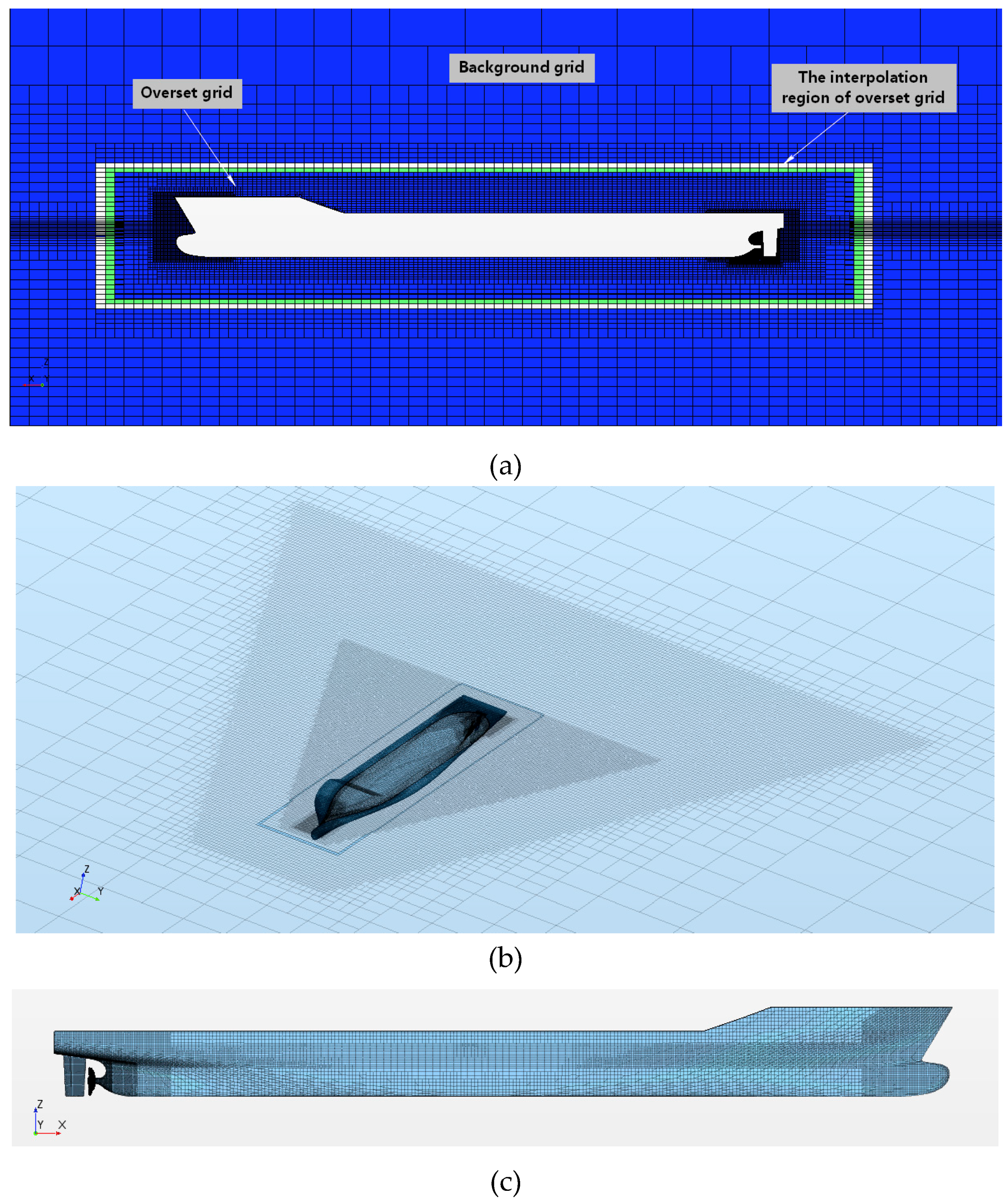
The hull motion is simulated by the overset grid method [17]. Compared to the general dynamic mesh, the overset grid is more adaptable and efficient in dealing with the large-amplitude motion. The overset grid method divides the computational domain into a number of subdomains whose grids are generated independently. Information transmission is implemented through grid nesting and overlap in these subdomains. In the boundary flow fields of the overset grids, information is coupled by interpolation. The overset grid generation involves two main steps: A hole-cutting operation on the grids of the background domain to shield the area inside the hole, mark those grids within the hole, and abandon them in the subsequent CFD computation; a point-searching operation to interpolate information transmitted at the hole boundaries for the subsequent numerical calculation. The schematic of overset grid is shown in Figure 1.
3. Calculation Modeling
3.1. Calculation Object
The standard model KCS container ship with the scale factor of 31.6 is used as the study objects as Figure 2 shows, whose principle parameters is listed in Table 1. The notable bulbous bow and stern extension may result in a complex wake and wave, which can provide a good wake environment to study the propeller exciting force characteristics. The propeller that goes with the ship is a KP505 propeller. The propeller principle parameters are given in Table 2.
3.2. Computational Domain and Boundary Condition
In order to simulate the hull motion, the computational domain is divided into the background domain and the overset grid domain as Figure 3 shows. The background domain is set as a cuboid water basin referring the towing tank. The inlet is 2 Lpp from the bow to ensure the inflow is uniform. The domain side and bottom from the hull surface are both 2 Lpp to avoid the hull flow field affected by the basin wall. Regarding the full development of the hull wake, the outlet from the stern is 3 Lpp. The inlet is set as a velocity inlet. The outlet is set as a pressure outlet. The domain top plane is set as symmetry and the other boundaries are set as a wall. The overset grid domain is nested in the background domain, which includes the hull-propeller-rudder model and can realize the simulation of the hull heave motion.
3.3. Grid Division
In our calculation, the trimmer mesh is used. It can capture the boundary layer flow effectively and control the total grid number of calculations. The grid division detail is shown in Figure 4. When performing the grid division, the grid size of the background domain around the overset area at best keeps the same with the grid size at the overset grid boundary. Furthermore, the motion range of the overset grid should be limited within the overset area. Regarding the hull surface mesh, more grids should be given to the bow and stern of the hull where the flow field varies dramatically. To capture the free surface better, the grids near the free surface and within the range of Kelvin waves are properly refined. The first layer of grids is 0.8–1 mm, corresponding to the Y plus which is approximately 60. Based on the previous analysis results of grid sensitivity [12], the total grids number is set as 4.5 million to save the computational time, but a satisfied calculation accuracy can also be reached.
3.4. Calculation Conditions and Setting of Motion Model
The research shows that the heave and pitch motion have the dominant influence on the propeller performance among the hull six degrees of freedom motion. It can even lead to propeller emergence and the racing phenomenon when the hull is in the large amplitude motion condition. Next, only the heave and pitch motion will be investigated in detail. The calculation is performed by two steps. At the first step, only the hull and rudder model are used to research the change rule of the propeller inflow in the heave and pitch motion. Then, the propeller is taken into consideration as a whole system to get the exciting force data in the heave, pitch motion and their couple motion. In this study, the hull motion is defined independently using the sinusoidal function as follows.
(1) Heave motion
Here, y is the moving distance of hull in the vertical direction, corresponding with the moving distance at z direction in the present calculating coordinate system and upward is positive. Ap is the amplitude of the heave motion and is selected as 0.25Tm and 0.125 Tm in the calculation by taking the amplitude of the forced oscillation model test as a reference. Tm represents the draft depth in the static water. is the frequency of heave motion and is dependent on the heave period Te. Te is selected as 2 s in this work. is the delay time to ensure the numerical stability, being selected as 26 s, at which the hull system is without the heave motion. The schematic plan of the heave motion rule is shown as Figure 5.
(2) Pitch motion
Here, is the pitch angle of the hull and it is defined as positive when the pitch is forward. Ap is the amplitude of the pitch motion and is selected as 2 degrees and 1 degree in the calculation. is the frequency of the pitch motion and is dependent on the pitch period Te. Te is selected as 2 s that is the same with the heave period. is also the delay time to ensure the numerical stability, being selected as 26 s. The schematic plan of the heave motion rule is shown as Figure 6.
The difficulty to simulate the motion of the hull-propeller system is how to realize the superimposition of the hull motion on the propeller rotating motion without the hull-propeller model separation showing in the process of the simulation. In order to handle this problem, the superimposed coordinate system method is applied. Therefore, three different coordinate systems are created, including the initial coordinate system, a new local hull coordinate system and a new local propeller coordinate system. The original point of the initial coordinate system is located in the crossing point of the after-perpendicular and free surface. The original point of the local hull coordinate system is located in the mass center of the hull. Its coordinates in its initial coordinate system are [3.532 m, 0.0, −0.111 m]. The original point of the local propeller coordinate system is located in the crossing point of the propeller axis and propeller disk. Its coordinates in the local hull coordinate system are [−3.404 m, 0.0, −0.113 m]. The initial direction of XYZ in these three different coordinate systems is the same. The details are shown in Figure 7. It can be seen that it is convenient to define the hull motion in the local hull coordinate system, as it is with the propeller’s rotation motion in the local propeller coordinate system. Then, the superimposed motion can be realized by attaching the locale propeller coordinate system to the hull motion in the local hull coordinate system.
4. Calculation Result Analysis
4.1. Validation of Calculation Method
Firstly, the numerical calculation for both the bare hull and hull-propeller-rudder system are performed without the hull motion to validate the calculation method with the condition [18] that the flow speed is 2.196 m/s, the propeller revolution speed is 9.5 rps and the draft is 0.3418 m. The time step is set as the time in which the propeller rotates for 4 degrees.
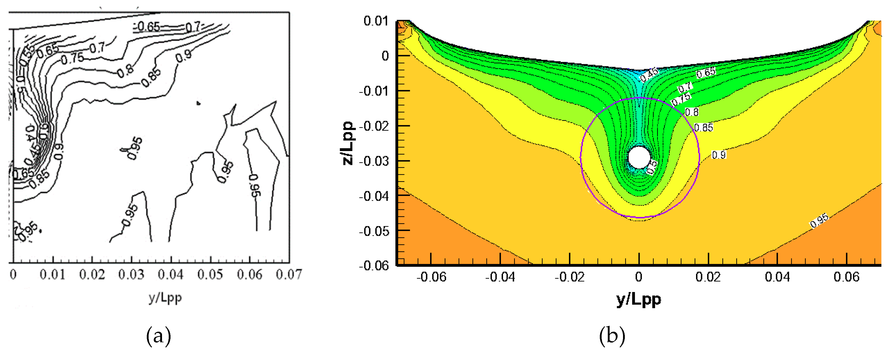
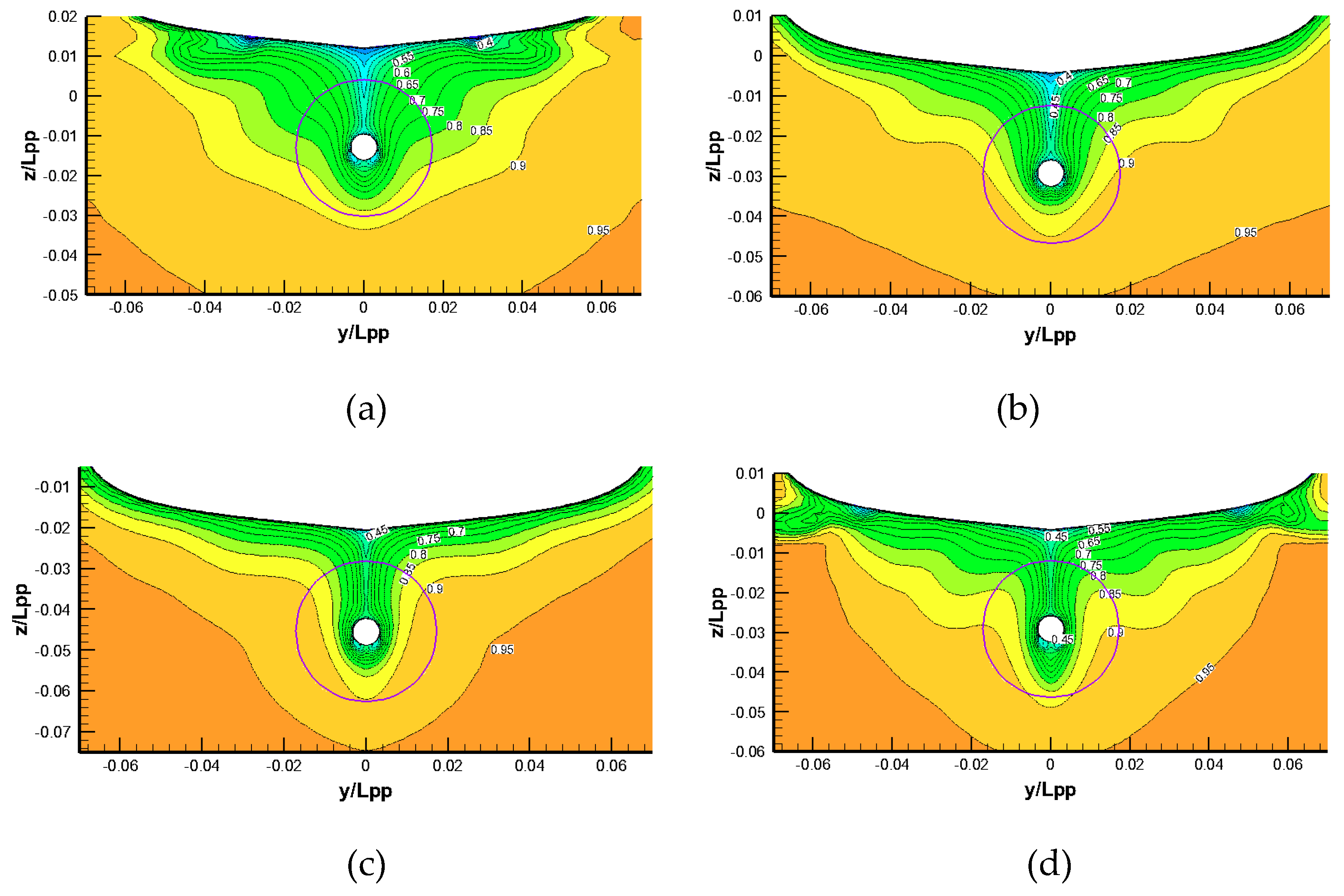
The Table 3 shows the hydrodynamic calculation results. In general, it shows good agreement with the experimental data [19]. The error of the propeller thrust is the biggest, but it is still under the 5% that can be accepted. The possible reasons for this are neglecting the hull posture change during the calculation and the presence of the rudder in this work. Figure 8 shows the comparison between EFD and CFD for the wave contour. It can be seen that the values and position of the peaks and troughs are consistent between EFD and CFD. The previous problems that the wave on the hull’s both sides dissipate too quickly and the details for the broken wave at the stern are not caught well and have been solved effectively by the logical grid division strategy. Figure 9 shows the comparison between EFD and CFD for the velocity contour. The calculated values also show good agreement with EFD’s. However, the shrinkage of the velocity contour of EFD towards the mid-ship section is more serious, that means the boundary layer is thinner in the experimental condition. The use of the boundary layer trip in test may cause this phenomenon happen. Overall, the calculation method used in this work is accurate and satisfactory.
4.2. Free Surface and Wake Analysis
4.2.1. Free Surface in Motion Condition
Figure 10 and Figure 11 show the wave patterns of the free surface at different times within a heave and pitch motion period. The wave pattern changes greatly with the time compared with it in the condition without the hull motion. The wave is generating and dissipating continuously due to the hull motion. It can be seen that, especially when the hull is heaving down or pitching up, the stern part becomes the main source to produce the wave because of the phenomenon of stern slapping water. From the viewpoint of energy, the wave costs the energy of the hull, therefore it will become the main reason to the growth of hull resistance in motion condition. As the hull moves periodically, the wave pattern on the hull’s two sides gradually spread out and finally form an obvious transverse wave alternating with peaks and troughs. Compared with the heave condition, the transverse wave in the pitch condition seems to develop more fully and distribute more regularly. Hence, it can be considered that the pitch case in our calculation influences the hull resistance more powerfully than the heave case.
4.2.2. Wake in Motion Condition
The propeller exciting force performance is strongly associated with the wake non-uniformity. When the ship sails normally without a large amplitude motion, the wake temporal non-uniformity induced by the flow turbulence characteristics is slight. The spatial wake temporal non-uniformity is the dominant factor affecting the propeller exciting force. However, when the ship sail in rough sea with a significant heave or pitch motion, the wake temporal non-uniformity caused by the motion period is non-negligible. The priority is given to the axial wake in the three directional wake. To analyze the non-uniformity of the axial wake, the axial velocity is non-dimensionalized by the inlet velocity (2.196 m/s). The spatial non-uniformity is defined as:
Here, is the dimensionless axial velocity. is the circumferential average of dimensionless axial velocity in a specific radius. is the peak value in a specific radius and is the valley value. is the spatial non-uniformity. The bigger the spatial non-uniformity is, the worse the propeller exciting force performance is expected to be. The temporal non-uniformity is defined as:
Here, is the disk surface average of the dimensionless axial velocity in a specific time. is the time average of the disk dimensionless axial velocity. is the temporal non-uniformity in a motion period which is defined similarly with the spatial non-uniformity.
Figure 12 shows the distribution of the nominal wake fields in the heave motion condition. At the time t = 0.25 Te, the velocity decreases dramatically as the hull rises to the highest position, corresponding with the propeller load becoming heavy. There is a rather strong vortex structure occurring on both sides of the hull bilge. At the time t = 0.75 Te, the velocity increase and its contour shrink to the hull obviously as the hull sinks to the lowest position, corresponding with the propeller load becoming light. Figure 13 shows the distribution of the nominal wake fields in the pitch motion condition. The wake is also strongly associated with the stern draught. The deeper the stern draught is, the bigger the velocity in the propeller plane can be.
Since the flow field at 0.7 R radius has a dominant influence on the propeller hydrodynamic performance, the spatial non-uniformity of the nominal wake is analyzed by taking the axial velocity at 0.7 R radius as a representation. The circumferential angle is defined as Figure 14. Figure 15 shows the circumferential distribution of axial velocity at different times. The analysis results of the spatial non-uniformity are listed at Table 4. In general, the hull heave or pitch motion does not make the spatial non-uniformity become worse. Reversely, there is some improvement at the time that the hull draft is deeper, for example when t = 0.75 Te.
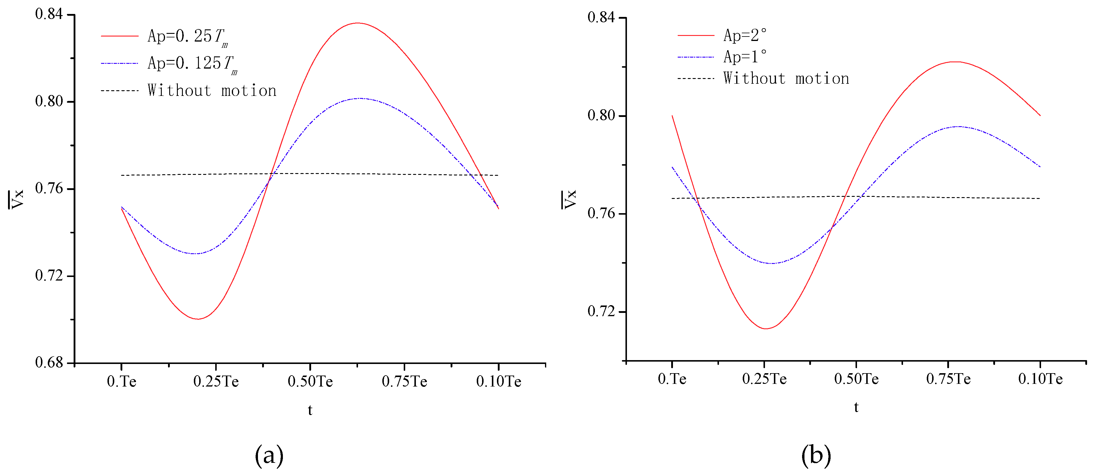
Figure 16 shows the average axial velocity curve at the disk plane in a motion period. From the analysis results listed in Table 5, compared with the condition without motion, the temporal non-uniformity of the heave increases sharply from 0.11% to 9.28% and 17.78% and the temporal non-uniformity of the pitch increases sharply from 0.11% to 7.28% and 14.17%. It also shows that the temporal non-uniformity has a significant positive relationship with the motion amplitude. The wake uniformity analysis is helpful to understand the change rule of the propeller exciting forcing in the motion condition later.
4.3. Hydrodynamic Performance Analysis
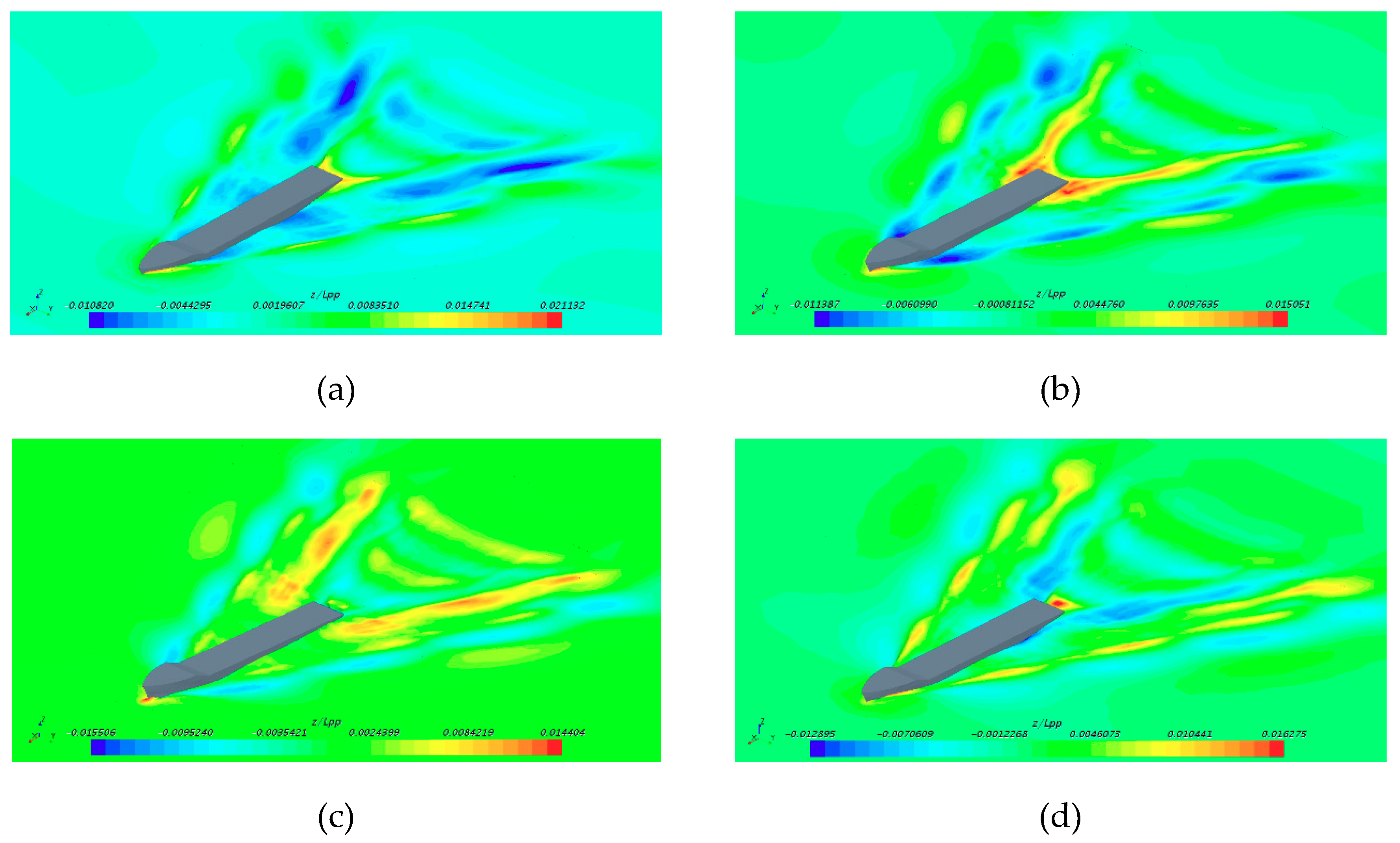
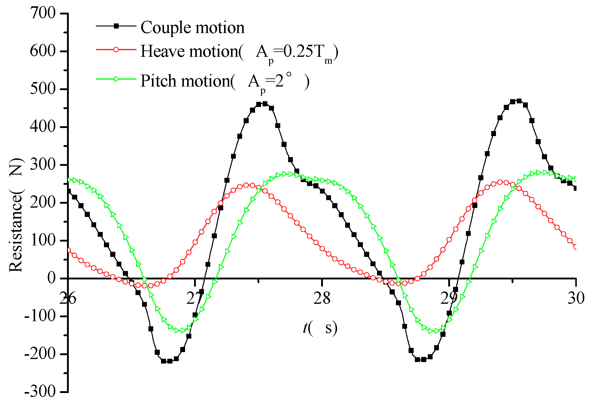
Table 6 lists the calculation results of the resistance. In the heave condition, the resistance increase percent is 54.23% when the heave amplitude is 0.25Tm and the resistance increase percent is 18.80% when the heave amplitude is 0.125Tm. In the pitch condition, the resistance increase percent is 69.66% when the pitch amplitude is 2° and the resistance increase percent is 20.68% when the pitch amplitude is 1°. As the motion amplitude become bigger, the resistance increases sharply. The resistance time average value in the couple motion condition is comparable with the single motion, but from the Figure 17, it can be seen that its amplitude of fluctuation is larger, which is unfavorable for the match of the ship-engine-propeller system. The growth of resistance mainly comes from the increase of the wetted surface area and residual resistance, which are induced by green water and wave making. Figure 18 has given the wave contour on the hull surface at a specific moment to show the change of the wetted surface area in different motion conditions.
Table 7 lists the calculation results of the propeller thrust. The drop of propeller thrust in the motion condition is remarkable. However, unlike the hull resistance, the thrust drop is not so sensitive with the motion amplitude. The difference between the time average thrust with different motion amplitude is very small. The decrease percent with the couple motion is comparable with a single motion, which is similar with the change rule of resistance. However, the amplitude of the thrust fluctuation in the couple motion is also larger, so the excitation from the propeller to the hull stern vibration is expected to be stronger. Figure 19 has shown the thrust change curves in the time domain.
4.4. Propeller Exciting Force Analysis
4.4.1. Propeller Bearing Force
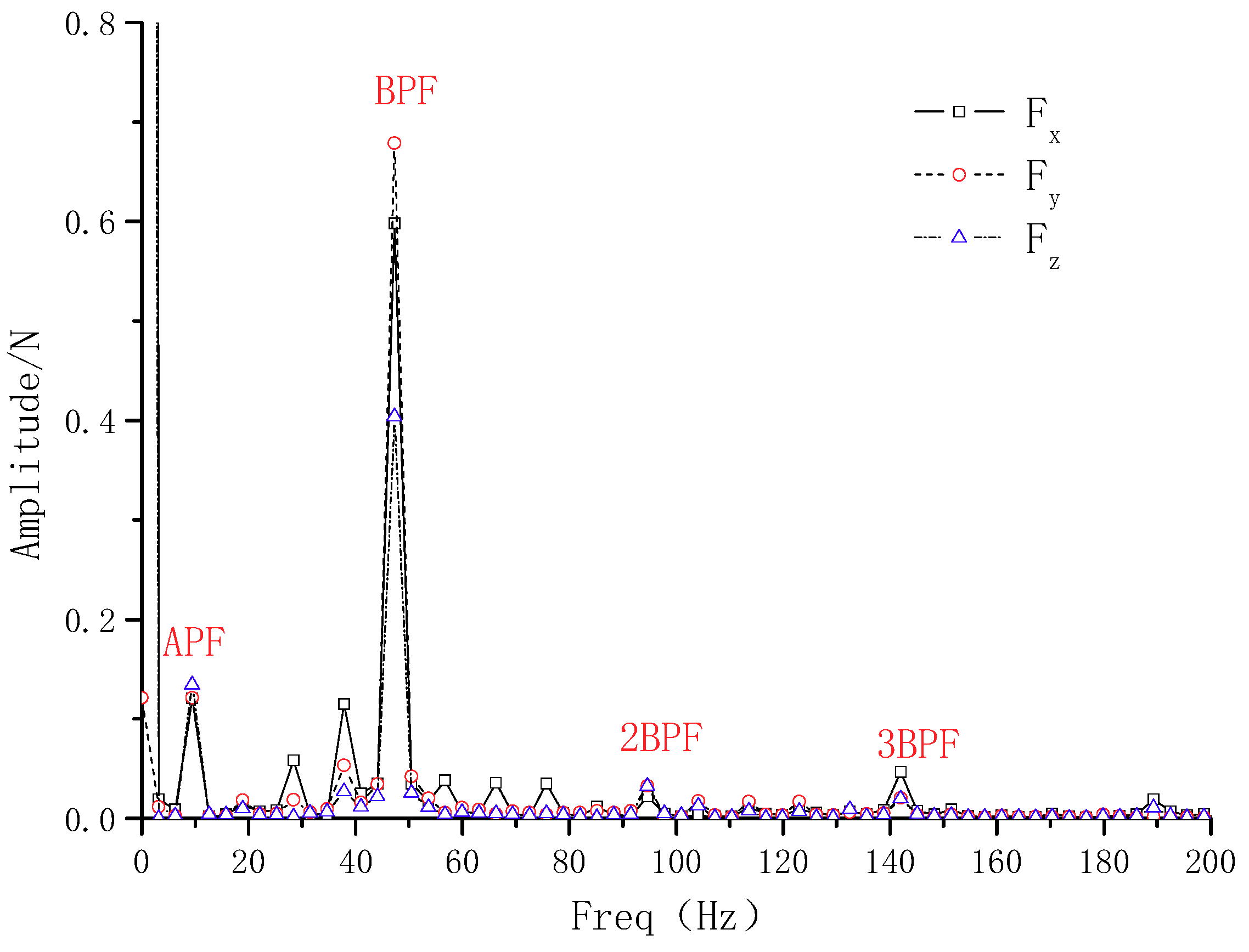
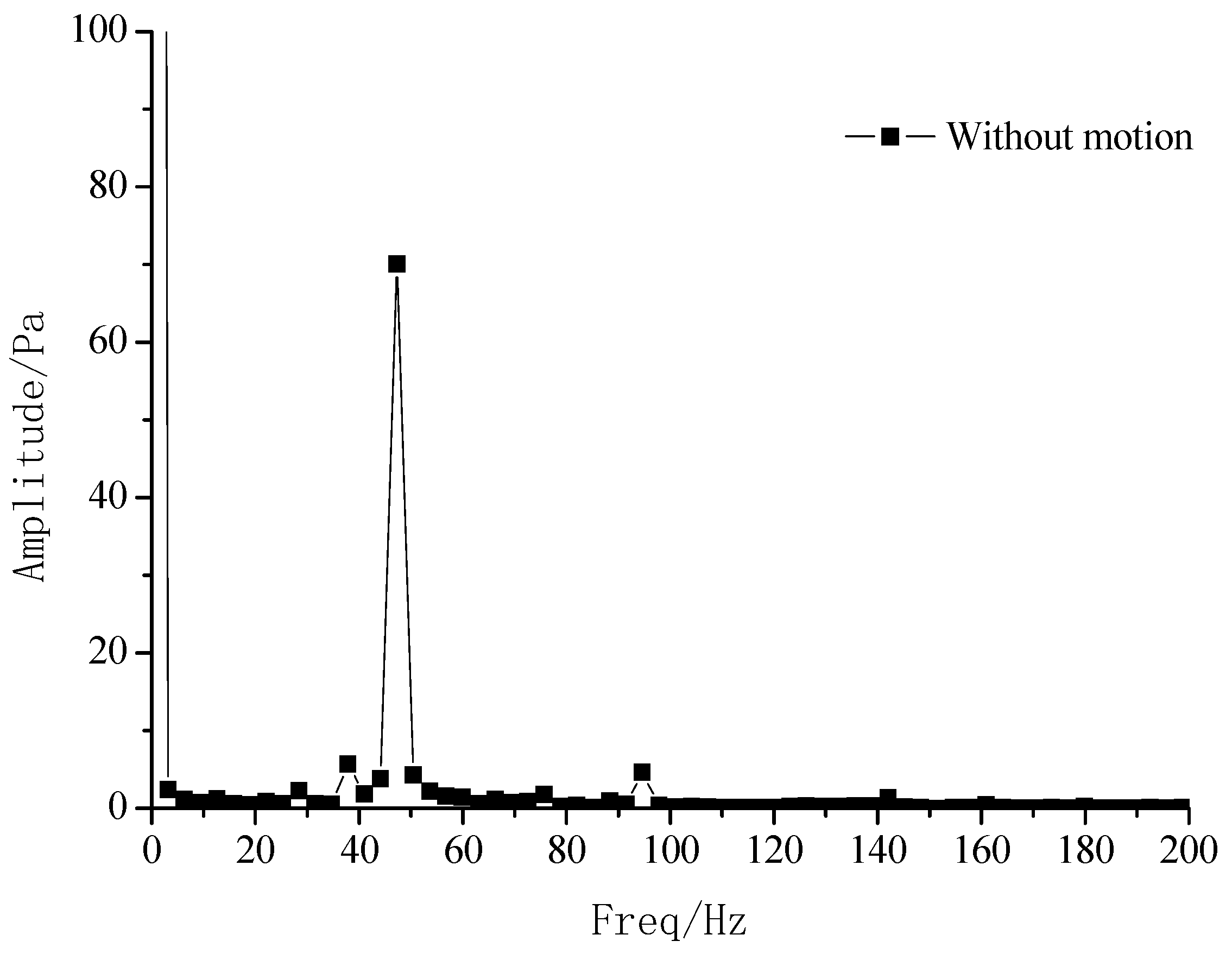
The propeller exciting force in the frequency domain was obtained after performing the FFT transform for the time domain signal. Figure 20 shows the frequency domain curves of the propeller exciting force without motion. Here, the Fx is the thrust, Fy is the horizontal force, Fz is the vertical force. It can be concluded that the propeller thrust and the side force have the same fluctuation frequency. The peaks appear at the axial frequency (9.5 Hz), the blade frequency (47.5 Hz), the double blade frequency (95.0 Hz) and the triple blade frequency (142.5 Hz), with the peak being the largest at the BPF and quickly attenuating afterwards. After 3 BPF, these forces can be ignored. The peaks between the thrust and side force do not show the obvious differences and that is because the propeller works in the non-uniform wake, the blades cannot balance the force in the Y, Z direction well. Although the time average of the side force is not very large, the fluctuating amplitude is comparable with the thrust.
Since the frequency domain characteristics of the side forces are similar with the thrust, only the domain curves of the thrust in the motion condition are given from Figure 21, Figure 22 and Figure 23. The other calculation results are listed in Table 8 and Table 9. Compared with the results without motion, the following rules can be concluded.
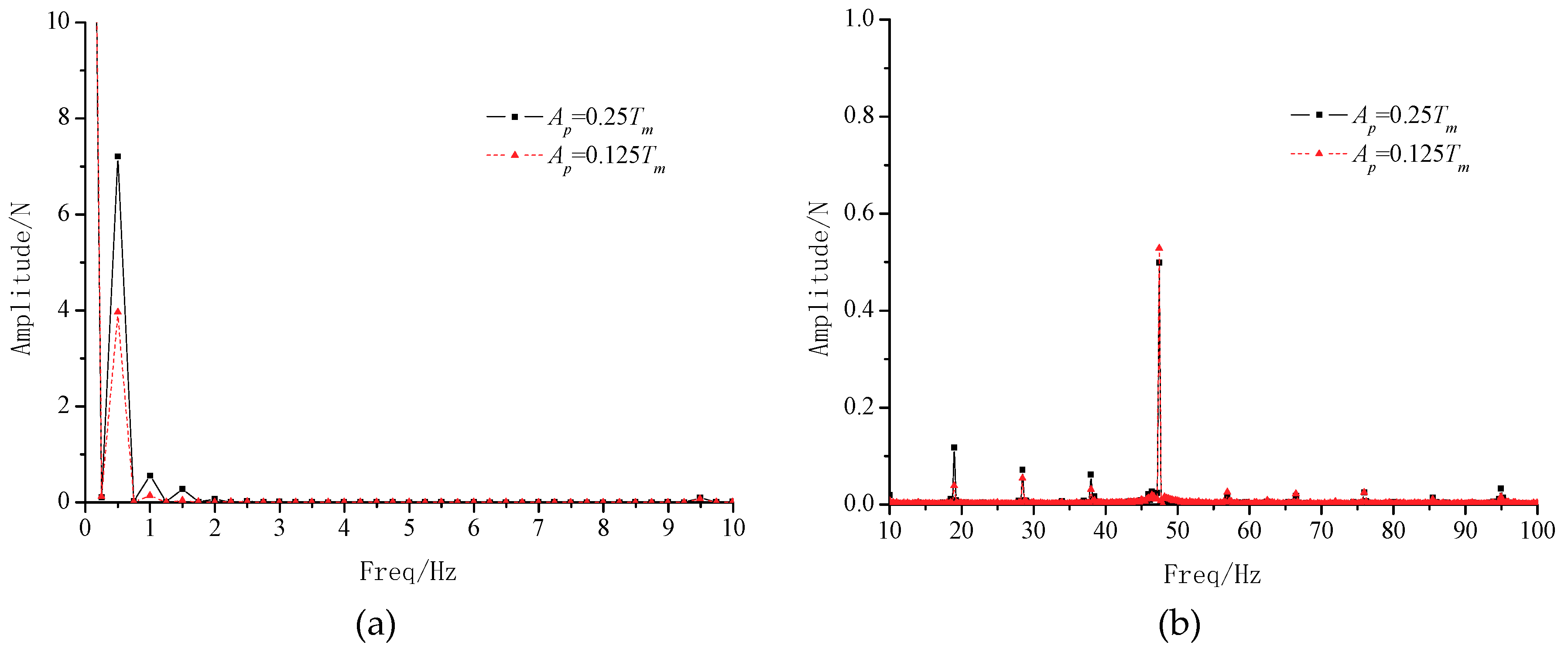
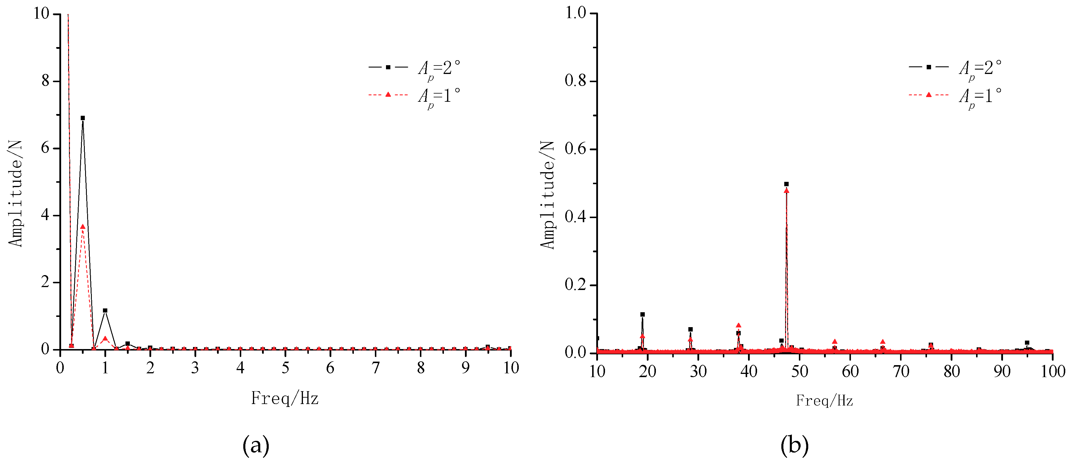
(1) Spectrum peaks are richer in the motion condition. The peaks show in motion frequency (0.5 Hz), double motion frequency (1.0 Hz) and triple motion frequency (1.5 Hz) to some degree besides the original blade frequency and axis frequency. (2) The peaks at the blade frequency that are induced mainly by the spatial non-uniformity at disk plane, is comparable with its value in the condition without motion. This rule corresponds with the wake analysis results that the hull motion does not have much influence on the spatial non-uniformity at a disk plane. (3) The peaks at a motion frequency which is induced mainly by the temporal non-uniformity at disk plane, is much bigger than its at blade frequency and it has become the main fluctuating quantity except for horizontal force. It means that temporal non-uniformity, compared with spatial non-uniformity, is the main factor that affects the propeller exciting force performance in the motion condition. Further, the side force peak at motion frequency is related with the hull motion direction. (4) The peak at the motion frequency shows linear dependence on motion amplitude and the larger the amplitude is, the higher the motion frequency peak can be. However, the peak at blade frequency is almost the same for different motion amplitudes. (5) The motion frequency peaks in couple motion is almost equal to the sum of the peaks in the heave and pitch condition. It means that the effect of the different hull motion acting on the propeller bearing force appears as linear superimposition.
4.4.2. Propeller-Induced Fluctuating Pressure
The fluctuation pressure measurement points are arranged referring to Figure 24 in the plane Z −0.04 m above the propeller. An analysis is undertaken of the characteristics of the propeller-induced hull surface fluctuating pressure in the motion condition by monitoring the time signal data of these five points from P0 to P4. An explanation is required in that the absolute coordinates of monitor point is changing during the hull motion, but its relative position to the hull and propeller always keeps the same.
The authors discovered that the characteristics of fluctuation pressure at different points is almost the same and only the peak values are different after analyzing the time signal data by FFT method. Another point that needs to be mentioned is that the distance from P0 point to the propeller tip is the shortest among these five points. There is no doubt that the peak value of fluctuating pressure in P0 point is maximum, which can show the fluctuating pressure level of the whole stern. Therefore, the figures from Figure 25, Figure 26, Figure 27 and Figure 28 just show the frequency domain curves of P0 point as representative to compare the characteristics of fluctuation pressure in different motion conditions.
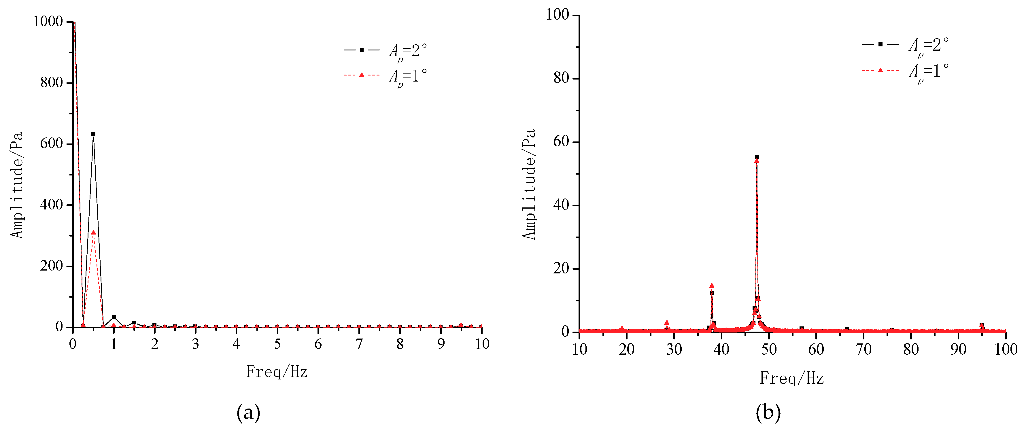
The spectrum peaks of P0 in the condition without motion mainly show in blade frequency (47.5 Hz), which is single compared with the condition with motion. The hull heave and pitch motion also excite the peaks in motion frequency (0.5 Hz) which is dominant among all the peaks. However, the value of the peaks in blade frequency does not show much difference during the motion. More attention should be paid to the peaks in the condition with the couple motion, unlike the single motion, in which the peaks associated with the motion frequency are aroused in a big range of frequency that is a quite difficult thing for the hull structure or equipment to avoid these characteristic frequencies. The fluctuating pressure is not only related to the excitation source of the propeller, but also highly related to the state of water medium between the propeller and hull surface. From the analysis results of the bearing force, the unsteady force of the propeller in the condition with couple motion mainly has a motion frequency component. Therefore, the possible reason for this phenomenon is that the superimposition of the heave and pitch motion has greatly changed the flow condition between the propeller and hull surface by different vortex structures and the generation of vortex structures are strongly related to the hull motion frequency.
In order to analyze the peaks of fluctuating pressure quantitatively, Figure 29 has given the peaks of every point at motion frequency and blade frequency for different conditions. It shows that when the motion amplitude is doubled, the peak value at motion frequency is also nearly doubled. The motion amplitude mainly influences the peaks associated with motion frequency rather than the peaks at blade frequency. This conclusion is consistent with the results given by the analysis of the wake and bearing force. However, unlike the bearing force, the peaks in the condition with the couple motion, which is at motion frequency or blade frequency, are greater than the sum of the peaks in the condition with the heave motion and pitch motion. It means that the couple motion can enlarge the fluctuating pressure in a single motion. Of course, it remains to be investigated how the fluctuating pressure will show if the motion frequency of the heave and pitch is not the same.
5. Conclusions
The numerical simulation has been conducted on the hull-propeller-rudder system of KCS model with the single and couple motion by employing the RANS method and overset grid method. Through the comparative analysis of hydrodynamic performance and the exciting force performance, the conclusions are obtained as follow.
(1) The calculation results without the hull motion are basically consistent with the experimental results, including the hydrodynamic performance of the hull-propeller–rudder system, the free surface wave contour and velocity contour in the propeller plane, which indicates that the calculation results are accurate and reliable.
(2) As the hull is in motion periodically, the wave pattern on the hull’s two sides gradually spread out and finally form an obvious transverse wave. When the hull is in the heaving down or pitching up stage, the stern part becomes the main source to produce the wave as it slaps against the water. The change of wave contour can become the main reason for the resistance increase. From the analysis of the wake field, it shows that the hull motion leads little changes to the disk wake spatial non-uniformity. However, the temporal non-uniformity in motion increases dramatically compared with case without motion.
(3) The increase of resistance and the drop of thrust induced by the hull motion are significant which can lead to obvious speed loss. In addition, when the motion amplitude becomes bigger, the resistance increases sharply. However, the thrust drop is not so sensitive. The time average value of resistance and thrust in the couple motion condition is comparable with the single motion, but their fluctuation value is much bigger.
(4) The spectrum peaks of the propeller bearing force are richer in the motion condition. Some peaks related to the motion frequency and its integral multiples are shown. The peak at heave frequency (0.5 Hz) is much bigger than the peak at blade frequency (47.5 Hz) and it has become the main fluctuating quantity, except for horizontal force. Furthermore, the motion frequency peak becomes bigger with the increase of motion amplitude. The motion frequency peaks in the couple motion are almost equal to the sum of the peaks in the heave and pitch condition. It means that the effect of the different hull motion acting on the propeller bearing force appears as linear superimposition.
(5) The characteristics of the propeller-induced fluctuating pressure in the frequency domain are similar with the bearing force. The different peaks associated with motion frequency are aroused in a big range of frequencies in the condition with the couple motion. The peaks, no matter which is at motion frequency or blade frequency, are greater than the sum of the peaks in the condition with the heave motion and pitch motion. It means that the couple motion can enlargement the fluctuating pressure in a single motion.
Our work only investigates the influence of the motion amplitude on the hydrodynamic performance of the hull-propeller-rudder system and propeller exciting force. The influence of the frequency and phase in the couple motion condition remain to be studied further. This is the point that our subsequent research will focus on.
Author Contributions
L.L. conducted CFD calculations and wrote original draft; B.Z. conducted the calculation results analysis; D.L. edited the paper; C.W. conducted some part of CFD calculations.
Funding
This research received no external funding.
Acknowledgments
At the beginning of this research, the help from Xiaoxing Peng to formulate the research idea is gratefully acknowledged.
Conflicts of Interest
The authors declare no conflicts of interest.
References
- van Sluijs, M.F. Performance and Propeller Load Fluctuations of a Ship in Waves; TNO 163S; Netherlands Ship Research Centre: The Netherlands, 1972. [Google Scholar]
- Jessup, S.D.; Boswell, R.J. The effect of hull pitching motions and waves on periodic propeller blade loads. In Proceedings of the 14th Symposium on Naval Hydrodynamics, Ann Arbor, MI, USA, 23–27 August 1982. [Google Scholar]
- Sasajima, T. Usefulness of quasi-steady approach for estimation of propeller bearing forces. In Proceedings of the Propellers Symposium Transactions SNAME, Virginia Beach, VA, USA, 1978. [Google Scholar]
- Breslin, J.P.; Andersen, P. Hydrodynamics of Ship Propellers, 1st ed.; Cambridge University Press: Cambridge, MA, USA, 1994. [Google Scholar]
- Politis, G.K. Simulation of unsteady motion of a propeller in a fluid including free wake modeling. Eng. Anal. Bound. Elem. 2004, 28, 633–653. [Google Scholar] [CrossRef]
- Yu, X. Research on Hydrodynamic Performance of Propeller in Heaving Condition. Master’s Thesis, Harbin Engineering University, Harbin, China, 2008. [Google Scholar]
- Carrica, P.M.; Fu, H.; Stern, F. Computations of self-propulsion free to sink and trim and of motions in head waves of the KRISO Container Ship (KCS) model. Appl. Ocean Res. 2011, 33, 309–320. [Google Scholar] [CrossRef]
- Sharma, A. Numerical Modeling of a Hydrofoil or a Marine Propeller Undergoing Unsteady Motion Via a Panel Method and RANS; Tech. Rep. 11-02; Department of Civil Engineering, UT Austin: Austin, TX, USA, 2011. [Google Scholar]
- Kinnas, S.A.; Tian, Y. Numerical modeling of a marine propeller undergoing surge and heave motion. Int. J. Rotating Mach. 2012, 2012, 257461. [Google Scholar] [CrossRef]
- Tezdogan, T.; Incecik, A. Full-scale unsteady RANS simulations of vertical ship motions in shallow water. Ocean Eng. 2016, 123, 131–145. [Google Scholar] [CrossRef] [Green Version]
- Lianzhou, W.; Chunyu, G. Numerical analysis of a propeller during heave motion in cavitating flow. Appl. Ocean Res. 2017, 66, 131–145. [Google Scholar]
- Sun, S.; Li, L.; Wang, C.; Zhang, H. Numerical prediction analysis of propeller exciting force for hull-propeller-rudder system in oblique flow. Int. J. Nav. Archit. Ocean Eng. 2017, 10, 69–84. [Google Scholar] [CrossRef]
- Li, L.; Zhou, B.; Liu, D.; Zheng, C. The numerical analysis of influence of the hull heave motion on the propeller exciting force characteristics. In Proceedings of the Sixth International Symposium on Marine Propulsors Smp’19, Rome, Italy, 27–30 May 2019. [Google Scholar]
- Wang, F. Principle and Application of CFD; Tsinghua University Press: Beijing, China, 2004; pp. 7–11. [Google Scholar]
- Menter, F.R. Two-equation eddy-viscosity turbulence models for engineering applications. AIAA J. 1994, 32, 1598–1605. [Google Scholar] [CrossRef] [Green Version]
- Karim, M.D.; Bijoy, P.; Nasif, R. Numerical simulation of free surface water wave for the flow around NACA 0015 hydrofoil using the volume of fluid (VOF) method. Ocean Eng. 2014, 78, 89–94. [Google Scholar] [CrossRef]
- Carrica, P.M.; Wilson, R.V. Ship motions using single-phase level set with dynamic overset grids. Comput. Fluids 2007, 36, 1415–1433. [Google Scholar] [CrossRef]
- Hino, T. Proceedings of the CFD Workshop; NMRI Report 2005; National Maritime Research Institute: Tokyo, Japan, 2005. [Google Scholar]
- Larsson, L.; Stern, F. CFD in Ship Hydrodynamics-Results of the Gothenburg 2010 Workshop. MARINE 2011. In IV International Conference on Computational Methods in Marine Engineering; Springer: New York, NY, USA, 2013; pp. 237–259. [Google Scholar]
Figure 1.
Schematic of overset grid.

Figure 2.
KCS ship and KP505 propeller geometry model.

Figure 3.
Computational domain and boundary condition: (a) Background domain and boundary condition; (b) Overset grid domain and hull-propeller-rudder model.
Figure 3.
Computational domain and boundary condition: (a) Background domain and boundary condition; (b) Overset grid domain and hull-propeller-rudder model.

Figure 4.
Computational grid distribution: (a) The distribution of overset grid; (b) The grids near the free surface; (c) Hull surface grids.
Figure 4.
Computational grid distribution: (a) The distribution of overset grid; (b) The grids near the free surface; (c) Hull surface grids.

Figure 5.
Schematic plan of heave motion rule.

Figure 6.
Schematic plan of pitch motion rule.

Figure 7.
Schematic plan of different coordinate systems.

Figure 8.
Comparison for wave contour: (a) Model test; (b) CFD calculation.

Figure 9.
Comparison for velocity contour (): (a) Model test; (b) CFD calculation.

Figure 10.
Free surface in a heave period (): (a) t = 0.25 Te; (b) t = 0.50 Te; (c) t = 0.75 Te; (d) t = 1.0 Te.
Figure 10.
Free surface in a heave period (): (a) t = 0.25 Te; (b) t = 0.50 Te; (c) t = 0.75 Te; (d) t = 1.0 Te.

Figure 11.
Free surface in a pitch period (): (a) t = 0.25 Te; (b) t = 0.50 Te; (c) t = 0.75 Te; (d) t = 1.0 Te.
Figure 11.
Free surface in a pitch period (): (a) t = 0.25 Te; (b) t = 0.50 Te; (c) t = 0.75 Te; (d) t = 1.0 Te.

Figure 12.
Distribution of the nominal wake fields in heave motion condition (, ): (a) t = 0.25 Te; (b) t = 0.50 Te; (c) t = 0.75 Te; (d) t = 1.0 Te.
Figure 12.
Distribution of the nominal wake fields in heave motion condition (, ): (a) t = 0.25 Te; (b) t = 0.50 Te; (c) t = 0.75 Te; (d) t = 1.0 Te.


Figure 13.
Distribution of the nominal wake fields in pitch motion condition (, ): (a) t = 0.25 Te; (b) t = 0.50 Te; (c) t = 0.75 Te; (d) t = 1.0 Te.
Figure 13.
Distribution of the nominal wake fields in pitch motion condition (, ): (a) t = 0.25 Te; (b) t = 0.50 Te; (c) t = 0.75 Te; (d) t = 1.0 Te.

Figure 14.
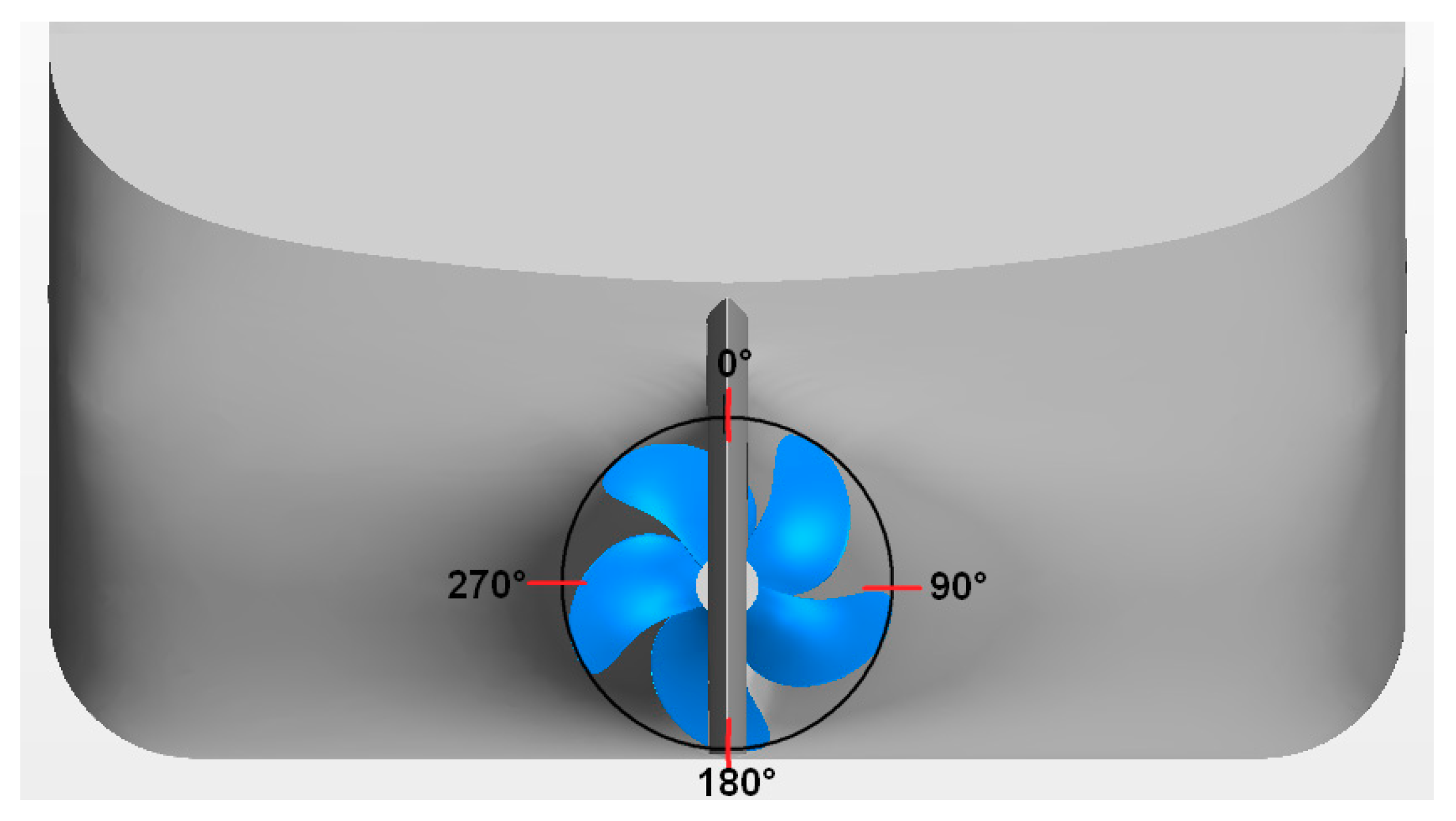
Definition of circumferential angle.

Figure 15.
Circumferential distribution of axial velocity at different time for 0.7 R radius: (a) Heave motion ; (b) Pitch motion .
Figure 15.
Circumferential distribution of axial velocity at different time for 0.7 R radius: (a) Heave motion ; (b) Pitch motion .

Figure 16.
Average axial velocity curves at disk plane in a motion period: (a) Heave motion; (b) Pitch motion.
Figure 16.
Average axial velocity curves at disk plane in a motion period: (a) Heave motion; (b) Pitch motion.

Figure 17.
Time domain curves of resistance for different motion condition.

Figure 18.
Wave contour on the hull surface at the specific moment: (a) Without motion; (b) Heave motion; (c) Pitch motion; (d) Couple motion.
Figure 18.
Wave contour on the hull surface at the specific moment: (a) Without motion; (b) Heave motion; (c) Pitch motion; (d) Couple motion.

Figure 19.
Time domain curve of thrust for different motion condition.

Figure 20.
Frequency domain curves of propeller exciting force without motion.

Figure 21.
Frequency domain curves of thrust with heave motion: (a) 0–10 Hz; (b) 10–100 Hz.

Figure 22.
Frequency domain curves of thrust with pitch motion: (a) 0–10 Hz; (b) 10–100 Hz.

Figure 23.
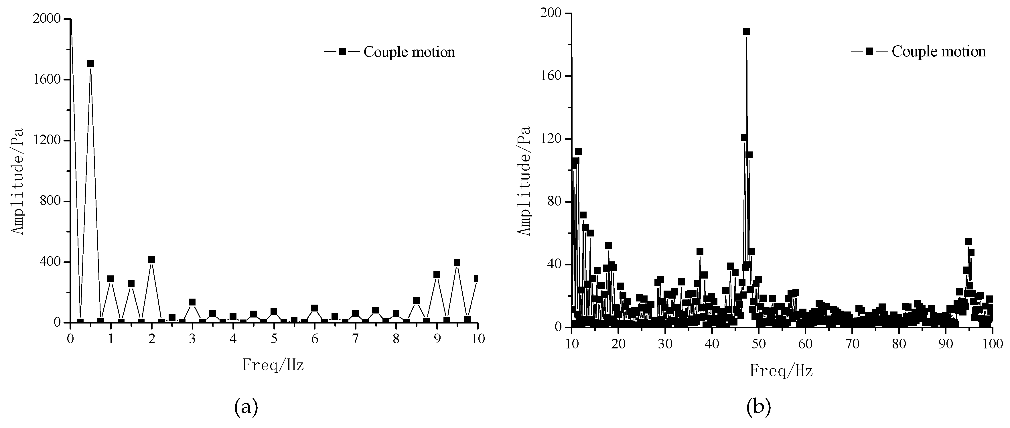
Frequency domain curves of thrust with couple motion: (a) 0–10 Hz; (b) 10–100 Hz.

Figure 24.
Arrangement of fluctuation pressure measurement points.

Figure 25.
Frequency domain curves of P0 point without motion.

Figure 26.
Frequency domain curves of P0 point in heave motion condition: (a) 0–10 Hz; (b) 10–100 Hz.
Figure 26.
Frequency domain curves of P0 point in heave motion condition: (a) 0–10 Hz; (b) 10–100 Hz.

Figure 27.
Frequency domain curves of P0 point in pitch motion condition: (a) 0–10 Hz; (b) 10–100 Hz.
Figure 27.
Frequency domain curves of P0 point in pitch motion condition: (a) 0–10 Hz; (b) 10–100 Hz.

Figure 28.
Frequency domain curves of P0 point in couple motion condition: (a) 0–10 Hz; (b) 10–100 Hz.
Figure 28.
Frequency domain curves of P0 point in couple motion condition: (a) 0–10 Hz; (b) 10–100 Hz.

Figure 29.
Fluctuation peaks at motion frequency (0.5 Hz) and blade frequency (47.5 Hz): (a) 0.5 Hz; (b) 47.5 Hz.
Figure 29.
Fluctuation peaks at motion frequency (0.5 Hz) and blade frequency (47.5 Hz): (a) 0.5 Hz; (b) 47.5 Hz.


Table 1.
Principle parameters of KCS model.
| Lpp (m) | 7.2786 |
|---|---|
| Draught (m) | 0.3418 |
| Wetted surface (m2) | 9.438 |
| Reynolds No. | 1.4 × 10⁷ |
| Froude No. | 0.26 |
Table 2.
Principle parameters of KP505 propeller model.
| Diameter (m) | 0.250 | Area Ratio | 0.70 |
|---|---|---|---|
| No. of blades | 5 | P/D (0.7R) | 1.00 |
| Hub ratio | 0.167 | Skew angle(°) | 12.66 |
Table 3.
Hydrodynamic calculation results of hull-propeller-rudder system.
| Description | Resistance/N | Thrust/N | Moment/N.m |
|---|---|---|---|
| CFD (with rudder) | 90.5 | 57.22 | 2.62 |
| EFD (without rudder) | 90.0 | 59.9 | 2.53 |
| Error | +0.56% | −4.47% | +1.58% |
Table 4.
Spatial non-uniformity of axial velocity at different time for 0.7 R radius.
| Condition | Without Heave | 0.25Te | 0.50Te | 0.75Te | 1.0Te | ||||
|---|---|---|---|---|---|---|---|---|---|
| Heave | Pitch | Heave | Pitch | Heave | Pitch | Heave | Pitch | ||
| Average value | 0.796 | 0.731 | 0.740 | 0.846 | 0.807 | 0.855 | 0.855 | 0.777 | 0.830 |
| Peak value | 0.868 | 0.808 | 0.830 | 0.915 | 0.891 | 0.913 | 0.916 | 0.847 | 0.897 |
| Valley value | 0.459 | 0.439 | 0.403 | 0.467 | 0.433 | 0.530 | 0.531 | 0.486 | 0.529 |
| Spatial non-uniformity (%) | 51.37 | 50.45 | 57.76 | 52.85 | 56.77 | 44.76 | 45.07 | 46.44 | 44.34 |
Table 5.
Temporal non-uniformity of axial velocity in a motion period.
| Condition | Without Motion | Heave | Pitch | ||
|---|---|---|---|---|---|
| Average value Peak value | 0.7666 | 0.7661 | 0.7677 | 0.7704 | 0.7689 |
| 0.7671 | 0.8361 | 0.8014 | 0.8221 | 0.7954 | |
| Valley value | 0.7663 | 0.6999 | 0.7301 | 0.7129 | 0.7394 |
| Temporal non-uniformity (%) | 0.11 | 17.78 | 9.28 | 14.17 | 7.28 |
Table 6.
Time average resistance for hull-propeller-rudder system.
| Condition | Without Motion | Heave | Pitch | Couple | ||
|---|---|---|---|---|---|---|
| Time average resistance (N) | 90.50 | 139.58 | 107.52 | 153.54 | 109.22 | 136.39 |
| Resistance increase percent (%) | - | 54.23 | 18.80 | 69.66 | 20.68 | 50.70 |
Table 7.
Time average thrust for propeller.
| Condition | Without Motion | Heave | Pitch | Couple | ||
|---|---|---|---|---|---|---|
| Time average thrust (N) | 57.22 | 33.31 | 34.50 | 32.94 | 34.35 | 33.76 |
| Thrust decrease percent (%) | - | −41.79 | −39.71 | −42.43 | −39.97 | −41.00 |
Table 8.
Peaks of horizontal force for different motion condition (unit: N).
| Condition | 0.5 Hz | 1.0 Hz | 1.5 Hz | 9.5 Hz | 19.0 Hz | 28.5 Hz | 47.5 Hz | |
|---|---|---|---|---|---|---|---|---|
| Without motion | - | - | - | 0.12 | 0.02 | 0.05 | 0.68 | |
| Heave | Ap = 0.25Tm | 0.62 | 0.2 | 0.06 | 0.34 | 0.02 | 0.04 | 0.75 |
| Ap = 0.125Tm | 0.33 | 0.06 | 0.01 | 0.36 | 0.04 | 0.04 | 0.73 | |
| Pitch | Ap = 2° | 1.04 | 0.16 | 0.05 | 0.35 | 0.02 | 0.04 | 0.76 |
| Ap = 1° | 0.51 | 0.08 | 0.02 | 0.37 | 0.03 | 0.05 | 0.71 | |
| Couple | 1.43 | 0.53 | 0.23 | 0.35 | 0.02 | 0.04 | 0.78 | |
Table 9.
Peaks of vertical force for different motion condition (unit: N).
| Condition | 0.5 Hz | 1.0 Hz | 1.5 Hz | 9.5 Hz | 19.0 Hz | 28.5 Hz | 47.5 Hz | |
|---|---|---|---|---|---|---|---|---|
| Without motion | - | - | - | 0.13 | - | - | 0.40 | |
| Heave | Ap = 0.25Tm | 2.44 | 0.11 | 0.08 | 0.36 | 0.03 | 0.02 | 0.46 |
| Ap = 0.125Tm | 1.265 | 0.03 | 0.01 | 0.38 | 0.01 | 0.01 | 0.58 | |
| Pitch | Ap = 2° | 3.00 | 0.18 | 0.07 | 0.35 | 0.03 | 0.02 | 0.50 |
| Ap = 1° | 1.43 | 0.06 | 0.02 | 0.40 | 0.01 | 0.01 | 0.47 | |
| Couple | 5.73 | 0.65 | 0.46 | 0.37 | 0.02 | 0.02 | 0.50 | |
© 2019 by the authors. Licensee MDPI, Basel, Switzerland. This article is an open access article distributed under the terms and conditions of the Creative Commons Attribution (CC BY) license (http://creativecommons.org/licenses/by/4.0/).
Share and Cite
MDPI and ACS Style
Li, L.; Zhou, B.; Liu, D.; Wang, C. Numerical Analysis of Influence of the Hull Couple Motion on the Propeller Exciting Force Characteristics. J. Mar. Sci. Eng. 2019, 7, 330. https://doi.org/10.3390/jmse7100330
AMA Style
Li L, Zhou B, Liu D, Wang C. Numerical Analysis of Influence of the Hull Couple Motion on the Propeller Exciting Force Characteristics. Journal of Marine Science and Engineering. 2019; 7(10):330. https://doi.org/10.3390/jmse7100330
Chicago/Turabian StyleLi, Liang, Bin Zhou, Dengcheng Liu, and Chao Wang. 2019. "Numerical Analysis of Influence of the Hull Couple Motion on the Propeller Exciting Force Characteristics" Journal of Marine Science and Engineering 7, no. 10: 330. https://doi.org/10.3390/jmse7100330
Note that from the first issue of 2016, this journal uses article numbers instead of page numbers. See further details here.