The Efficient Application of an Impulse Source Wavemaker to CFD Simulations


1
Marine Research Group, Queen’s University Belfast, Belfast BT22 1RQ, UK
2
Centre for Ocean Energy Research, Maynooth University, W23 Maynooth, Co. Kildare, Ireland
3
Department of Fluid Mechanics, Faculty of Mechanical Engineering, Budapest University of Technology and Economics, H-1111 Budapest, Hungary
*
Author to whom correspondence should be addressed.
J. Mar. Sci. Eng. 2019, 7(3), 71; https://doi.org/10.3390/jmse7030071
Submission received: 21 January 2019
/
Revised: 9 March 2019
/
Accepted: 12 March 2019
/
Published: 19 March 2019
(This article belongs to the Special Issue Advances in Marine Dynamic Simulation)
Abstract
:Computational Fluid Dynamics (CFD) simulations, based on Reynolds-Averaged Navier–Stokes (RANS) models, are a useful tool for a wide range of coastal and offshore applications, providing a high fidelity representation of the underlying hydrodynamic processes. Generating input waves in the CFD simulation is performed by a Numerical Wavemaker (NWM), with a variety of different NWM methods existing for this task. While NWMs, based on impulse source methods, have been widely applied for wave generation in depth averaged, shallow water models, they have not seen the same level of adoption in the more general RANS-based CFD simulations, due to difficulties in relating the required impulse source function to the resulting free surface elevation for non-shallow water cases. This paper presents an implementation of an impulse source wavemaker, which is able to self-calibrate the impulse source function to produce a desired wave series in deep or shallow water at a specific point in time and space. Example applications are presented, for a Numerical Wave Tank (NWT), based on the open-source CFD software OpenFOAM, for wave packets in deep and shallow water, highlighting the correct calibration of phase and amplitude. Furthermore, the suitability for cases requiring very low reflection from NWT boundaries is demonstrated. Possible issues in the use of the method are discussed, and guidance for accurate application is given.
1. Introduction
While CFD enables the simulation of complex flow phenomena, such as two-phase flows and gravity waves, setting up a simulation of coastal or marine engineering processes, with correct wave creation and minimum reflection, can be a challenge. A wide range of Numerical Wavemaker (NWM) methods exist in the literature for the generation and absorption of waves in a CFD simulation. Wave generation methods can be broadly grouped into two main categories:
- Replication of physical wavemakers, such as oscillating flaps, paddles or pistons
- Implementation of numerical/mathematical techniques, introducing source terms or similar into the governing equations
The first category of wave generation methods directly simulates the wavemaker by a moving wall, requiring mesh motion/deformation in the CFD domain [1], which can be a complex and computationally-expensive task. Additionally, because these methods replicate the real processes in a physical laboratory tank, they also incur the well-known drawbacks of physical wavemakers encountered in an experimental facility, such as evanescent waves, imperfect wave absorption and the required implementation of a wavemaker control system. Another drawback of conventional wave pistons is that they are typically limited to low order waves (first or second order).
In contrast to directly mimicking physical wavemakers, the second category of wave generation methods is generally more computationally efficient, using numerical algorithms to create the desired flow conditions by manipulating the field variables. In principle, there are four types of methods in the second category of wave generators:
Correspondingly, wave absorption can also be achieved using a number of methods. The trivial solution, of using a very long tank and limiting the simulation duration to a small number of wave cycles, is certainly not efficient or elegant and will therefore not be considered herein. The relaxation and boundary wave generation methods allow for wave absorption to be achieved actively by the NWM, whereas the mass and impulse source function methods can be used in combination with numerical beaches to dissipate waves and eliminate reflections.
While a comparison of different wavemakers is not within the scope of this paper, and has been addressed by Windt et al. [19], we want to highlight some common issues in NWTs. Wavemakers relying on open boundaries or algorithms that set the species variable, such as relaxation methods, are not necessarily mass conservative. Compared to an experimental facility, where waves are typically created in an enclosed volume of water, wave run-up along a sloping bottom, for example, might not be recreated correctly. Numerical beaches, while in many cases expected to be more computationally expensive than boundary conditions, are able to absorb waves to any desired level of reflection. The user thus has the possibility to balance computational burden against permissible reflections. Mass source methods are very similar to impulse source methods, but problems can arise when generating waves of significant height in shallow water. Once the surface level falls below the source region, wave generation fails. It should be noted that, at the wavemaker location, the surface elevation is twice the wave amplitude of the target wave train, since two wave trains travelling in opposite directions are created. The present paper thus focuses on the impulse source wavemaker.
1.1. Impulse Source Wavemaker
The difficulty in utilising an impulse source as an NWM lies in calculating the required source function to obtain a desired target wave series. Since the free surface is not a variable in the RANS equations, there is no direct expression relating the impulse source function to the resulting generated wave series. However, for depth-integrated equations, the free surface does appear as a variable, which Wei et al. [20] utilised to derive a transfer function between the source amplitude and the surface wave characteristics, generating mono- and poly-chromatic waves in Boussinesq-type wave models. Following this approach, generating waves by manipulating the impulse term in the Navier–Stokes equation has successfully been applied to shallow water waves in CFD simulations by Choi and Yoon [18] and Ha et al. [15]. Ha et al. [15] describe several issues, especially when creating deep water waves, originating from the Boussinesq simplifications used in the source term derivation. They also discussed limitations inducing numerical errors when applying a momentum source function to random wave generation. Despite those promising first steps, internal wavemakers have not seen widespread application.
In theory, limitations due to the Boussinesq simplification might be overcome by employing stream functions or other high order wave theories. In practice, evaluating higher order wave theories at multiple spatial positions (across all faces of the patch or all cells in the wavemaker region) can be computationally expensive. Furthermore, in many practical CFD applications, the accurate wave trace description is required at some distance away from the wave maker, typically in the middle of the domain. Schmitt [21] presented some progress in the use of neural networks for calibrating extreme waves in shallow water conditions, and another interesting application of two internal wavemakers in a single NWT in deep and intermediate water can be found in McKee et al. [22].
The present paper follows an alternative, more generalised, method to determine the required source function. The proposed method follows from standard calibration procedures utilised for physical wavemakers in real wave tanks, which iteratively tune the input signal applied to the wavemaker, in order to minimise the error between the measured and targeted wave series. Unlike previous methods to determine the source function, which are restricted to shallow water waves, the method proposed herein is applicable from deep to shallow water conditions, able to generate any realistic wave series at any desired location in an NWT, without explicitly employing any wave theory. Additionally, while dissipation can reduce a theoretically-correct wave height from the source region as it travels to the target location, the proposed method overcomes this problem since it is designed to obtain the desired wave signal at the target location.
Iterative calibration methods will of course increase the computational burden when compared directly to an analytically-derived accurate wavemaker function. However, by performing the calibration runs on a two-dimensional slice, the computational overhead is almost negligible compared to fully-three-dimensional simulations of realistic test cases. For many scientific or industrial applications, wavemakers with sophisticated theoretical solutions are used, although transient time traces require calibration, practically making the details of the wavemaker transfer function irrelevant and even creating an unnecessary overhead [23]. Applying a calibrated two-dimensional result to a corresponding three-dimensional domain is efficient and is also the recommended approach by Perić and Abdel-Maksoud [24].
The paper will demonstrate that, by utilising the proposed method, the source function can consist of a purely horizontal impulse component that varies in time. The time evolution of the magnitude and direction of this simple impulse source term can be calibrated using a standard spectral analysis method, which is commonly used in physical wave tanks. The remaining parameters of the impulse source wavemaker that need to be chosen are then the geometrical size and shape of the source function inside the NWT domain. An investigation of the effect of these geometric parameters will be presented to offer guidance on the selection of those values.
1.2. Outline of the Paper
The remainder of the paper is organised in the following four sections. In Section 2, the implementation of the impulse source wavemaker and the theoretical background is discussed in detail. The following two sections then present the application of the impulse source wavemaker to a wave packet in deep and shallow water conditions, with Section 3 detailing the particulars of the case study and Section 4 presenting the results and a discussion. Finally, in Section 5, a number of conclusions are drawn.
2. Implementation
This section details the implementation of the impulse source wavemaker, within a CFD solver, based on RANS models. First, the modification of the impulse equation to produce the wavemaker is detailed. Next, the definition of the parameter values, associated with the modified impulse equation, is discussed. Finally, the calibration procedure used to generate a target wave at a specified location is presented.
2.1. The Impulse Equation
A Volume Of Fluid (VOF) RANS model for incompressible flow includes the following impulse equation:
where t is time, the fluid velocity, p the fluid pressure, the fluid density, the stress tensor and the external forces, such as gravity. The stress tensor can include terms from a turbulence model; however, for this paper, all cases presented use a laminar flow model, since only non-breaking waves are considered. The proposed impulse source wavemaker is implemented by adding two terms to Equation (1):
- : This is the source term used for wave generation, where r is a scalar variable that defines the wavemaker region and is the acceleration input to the wavemaker at each cell centre within r. r is dimensionless, while is given in the units of .
- : This describes a dissipation term used to implement a numerical beach, where the variable field controls the strength of the dissipation, equalling zero in the central regions of the domain where the working wavefield is required and then gradually increasing towards the boundary over the length of the numerical beach [25]. is given in units of .
Introducing these two terms to Equation (1) yields the adapted impulse equation:
2.2. Setting Parameter Values
The values for the parameter fields r and are set during preprocessing, and their definition is crucial for the correct functioning of the method.
- r is set to one in the region where the wavemaker is acting and zero everywhere else in the NWT domain. Therefore, the size of the wavemaker and its position within the NWT must also be selected. To offer guidance on the selection of the wavemaker size and position, the case study presented in Section 3 and Section 4 investigates the effect of these parameters on the wavemaker performance.
- is initialised using an analytical expression relating the value of and the geometric coordinates of the NWT. The simplest expression would be a step function, where the value of is constant inside the beach and is zero everywhere else in the NWT. However, such a sharp increase in the dissipation will cause numerical reflections. Instead, the value of should be increased gradually from the start to the end of the numerical beach. Equation (3) is used in the current implementation, which has been shown to result in sufficient absorption [25]:where is the length of the numerical beach, x is the position within the numerical beach, equalling zero at the start and increasing to at the NWT wall, and stands for the maximum value of . Guidance on the selection of the parameters and is also given in the case study (see Section 3.4.4).Perić and Abdel-Maksoud [26] recently derived an analytical solution describing the ideal setting for and validated the method in a numerical experiment, removing the need for parameter studies in the future.
2.3. Calibration Procedure
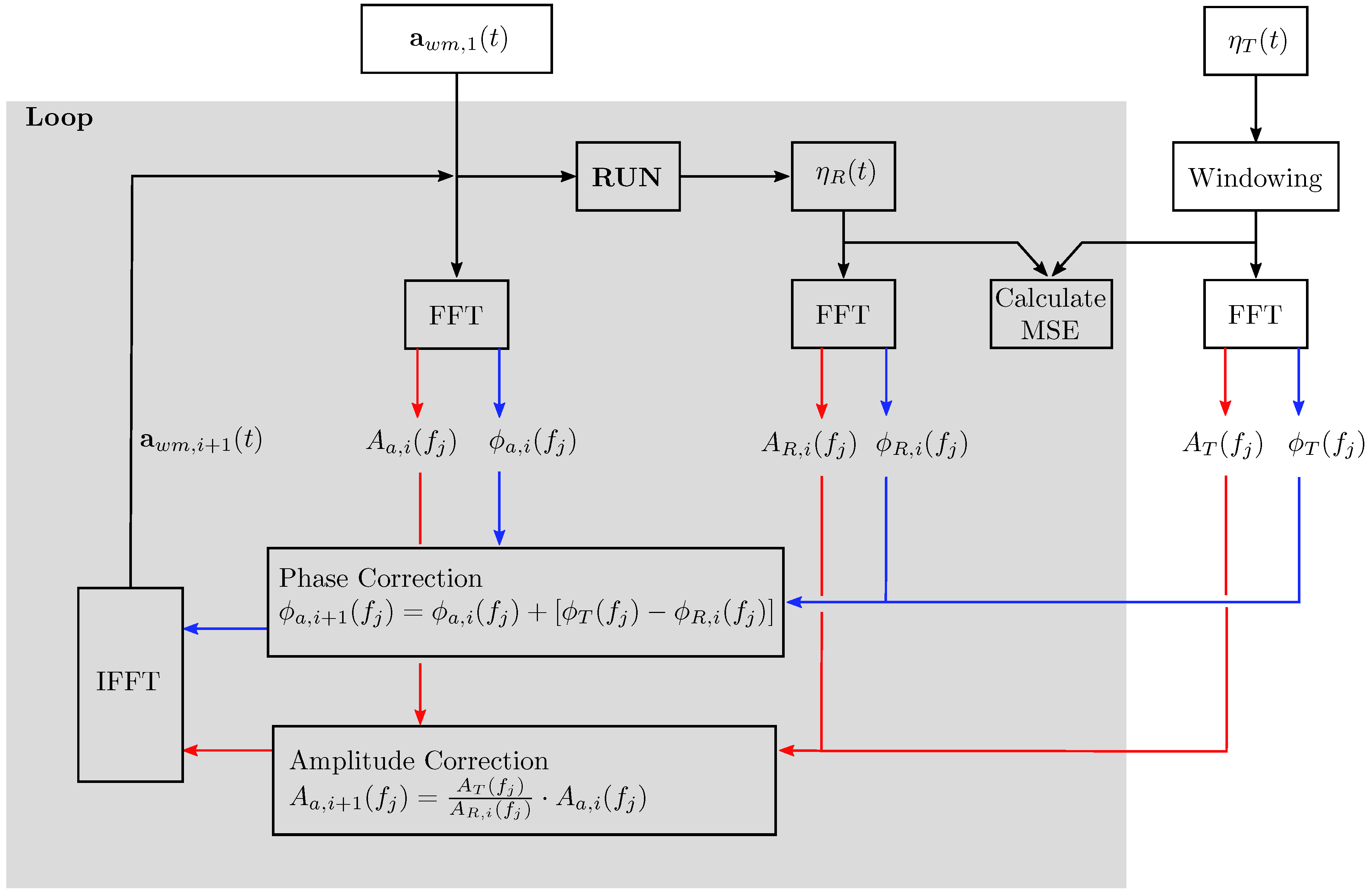
The source acceleration time trace, , is calibrated, using a standard spectral analysis method, based on work presented by Masterton and Swan [27], to produce a target wave series at a desired position within the NWT. Figure 1 shows a schematic of the calibration procedure, which comprises the following steps:
- Define target wave series at desired NWT location, , with a signal length and samples
- Perform a Fast Fourier Transform (FFT) on , to obtain the amplitudes, , and phase components, , for each frequency component, , with , where
- Generate an initial time series for the wavemaker source term, (can be chosen randomly or informed by )
- Perform an FFT on , to obtain the amplitudes, , and phase components, , for each frequency component of the input source term
- Run the simulation, for iteration i, using the wavemaker source term , and measure the resulting free surface elevation at the chosen NWT location,
- Perform an FFT on , to obtain the amplitudes, , and phase components, , for each frequency component of the generated wave series
- Calculate the new amplitudes for each frequency component of the input source term, , by scaling the previous amplitudes, , with the ratio of target surface elevation amplitude, , and the generated surface elevation amplitude from the previous run, :
- Calculate the new phase components, , by summing with the difference between the target elevation phase, , and the measured surface elevation phase from the previous run, :
- Generate the new time series for the wavemaker source term, , by performing an inverse Fourier transform on and
- Repeat Steps 5–9 until either a maximum number of iterations or a threshold for the Mean-Squared Error (MSE) between the target and resulting surface elevation is reached.
It should be noted that, although the method is based on the work described by Masterton and Swan [27], we have further simplified it. Instead of evaluating the phase-shift caused by the distance between the wavemaker and the point of interest, which would require the use of some wave theory to find the wavenumber k, here, the phase between the wavemaker and the target is directly adjusted (Step 8).
2.4. Calibration Procedure for Regular Waves
The calibration method detailed above might fail to resolve the single peak in the frequency domain for short time traces of regular waves. At the same time, in regular waves, the phase of the wave is generally not of interest, allowing for a simplification of the calibration. Schmitt and Elsaesser [28], Schmitt et al. [29], Vorhoelter et al. [30] and Windt et al. [19] used the same solver formulation and simply tuned the amplitude of an oscillating source to create monochromatic waves of a desired height. The following calibration method is used for regular waves:
- The source term is set to oscillate in the horizontal direction with the desired wave frequency.
- The amplitude is initialised with an arbitrary value.
- After the initial, and each subsequent run, the surface elevation is analysed in the time domain. The mean is removed from the surface elevation. The mean wave height, , is then obtained as the difference between the mean of the positive and mean of the negative peaks.
- A new wave maker amplitude, , is obtained by linearly scaling the previous value with the ratio of target and resulting wave height, , as follows
Steps 3 and 4 are repeated until the desired wave height is achieved.
3. Case Study
In this section, a case study is presented with two main objectives: firstly, to demonstrate the capabilities of the impulse wavemaker and the self-calibration procedure in producing realistic deep, intermediate or shallow water wave series, at a specified location in a wave tank. The second objective is to provide guidance on the selection of the wavemaker source region, by investigating the effect that the size and position of the source region has on the resulting waves. It might be expected that a very long source area will decrease accuracy, whereas a very short source region will require very large velocity components to create a target wave. For the shallow water impulse wavemaker presented by Choi and Yoon [18], a source length of about a quarter to half a wavelength is recommended. In shallow water, the entire water column, from the sea floor up to the water surface, performs an oscillating motion, whereas in deep water, only part of the water column is affected, and the wave motion does not extend to the sea floor. It is thus an interesting question how to choose the length and depth of the source region to achieve optimal results.
3.1. Target Waves
The case study considered two types of target waves, multi-frequency and regular waves, to demonstrate the calibration procedures outlined in Section 2.3 and Section 2.4, respectively.
3.1.1. Multi-Frequency Wave Packet
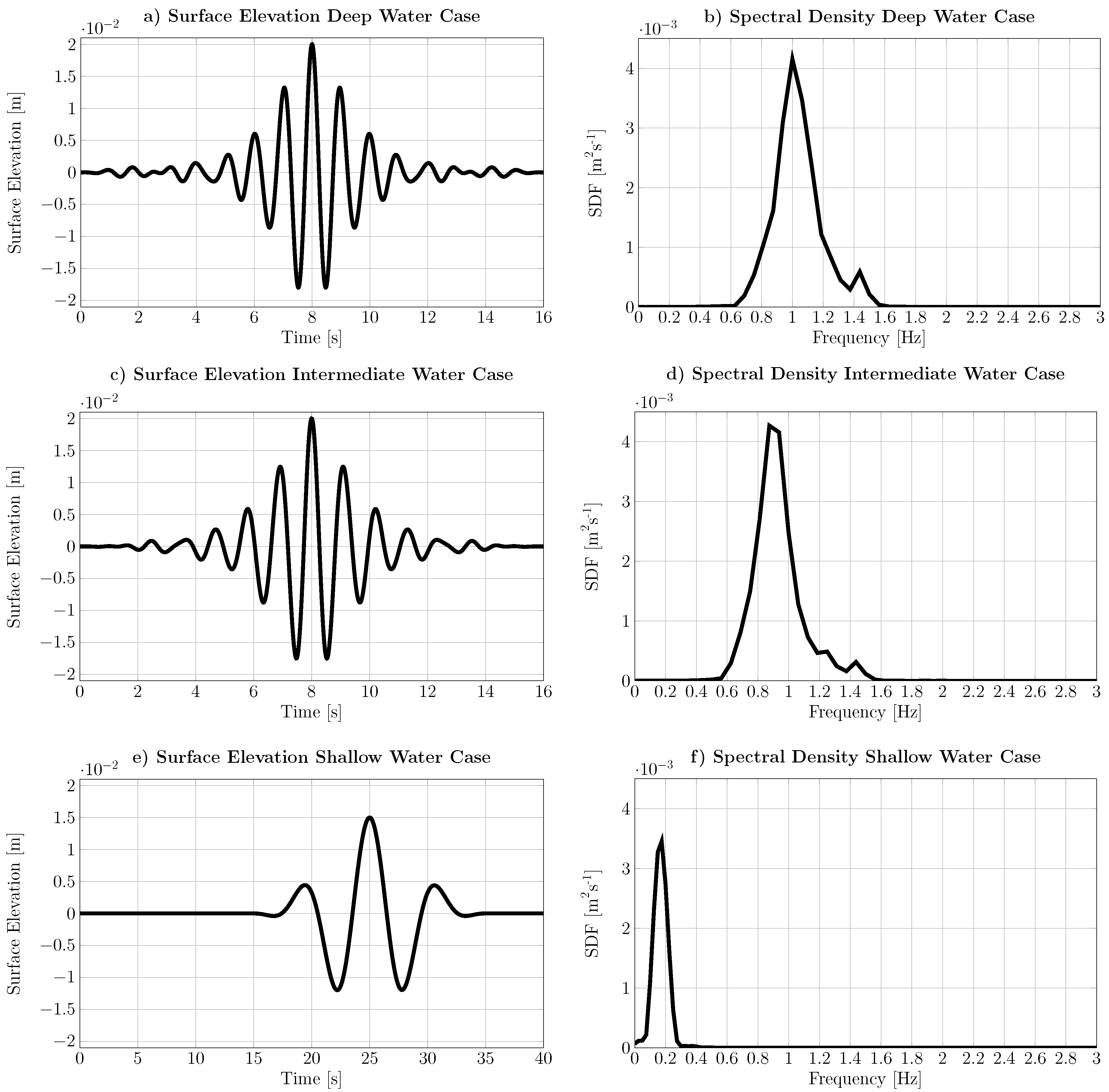
To demonstrate the ability of the impulse wavemaker, the case study created a unidirectional multi-frequency wave packet at a specified location in the NWT. The wave packet considered was a realisation of the NewWave formulation as presented by Ning et al. [31]. A NewWave wave packet comprises a summation of all the frequency components of a given spectrum, such that the largest amplitude wave crest is created in the temporal centre of the packet. The governing equations for the surface elevation, , and amplitude of each wave component, , with , are given in Equations (4) and (5), respectively:
In Equation (4), represents the spatial focal location and the temporal focal instant. In Equation (5), is the spectral density and the frequency step. represents the amplitude of the largest wave crest.
For this case study, three different wave packets, for deep, intermediate and shallow water conditions, were considered. The wave characteristics for the different waves are listed in Table 1.
Although the parameters used in this case study were, to a certain extent, arbitrarily chosen, wave packets are generally well suited for testing the calibration of amplitudes and phases of different frequency components [32] and are also of practical relevance in industrial applications [33]. While for the deep and intermediate water case, the wavelength was kept constant, the water depth was equal for the deep and shallow water case. Choosing the parameters for the shallow water case requires care, in order to avoid breaking waves. Time traces for the surface elevation, , and plots of the spectral density, , are shown in Figure 2, for all three wave packets.
3.1.2. Regular Waves
Two cases demonstrating the creation of regular waves in intermediate and deep water are presented. The target wave height was set to m and the period to s for the shallow water case and s for the deep water case, replicating the peak frequency and maximum wave height of the corresponding wave packets described in Section 3.1.1. If not mentioned specifically, the settings, found to be suitable for the corresponding wave packets, have been used for the setup of these regular wave cases.
3.2. Source Region
A rectangular-shaped source region was used for all simulations. Length L, height H and positions were varied to investigate the effect of the source region shape and position on the wave maker performance.
3.3. Simulation Platform
The NWT implementation for this case study was based on the interFoam solver from the OpenFOAM toolbox. The interFoam solver uses a VOF approach for modelling the two different fluid phases, air and water, in order to capture and track and the free surface. More details on this solver were presented by Rusche [34]. Although the case study employed OpenFOAM as the CFD solver, the method can easily be applied to any CFD software that allows user coding. For example, Choi and Yoon [18] implemented the shallow water impulse source wavemaker in ANSYS Fluent, using its user-defined functions capability.
The calibration function was implemented in the free scientific programming software, GNU Octave [35]. This results in all of the software utilised in this case study being open-source or free. The source code for the case study setup and implementation has been shared by the authors on the CCP-WSIrepository [36], allowing anyone to access and utilise the developed impulse source wavemaker easily.
3.4. Numerical Wave Tank Setup
Since the case study considered a unidirectional input wave, a Two-Dimensional (2D) NWT was implemented to simplify the setup and reduce computational overheads. The NWT setup is described below, detailing the geometry, boundary conditions, mesh and calibration of the absorption beach.
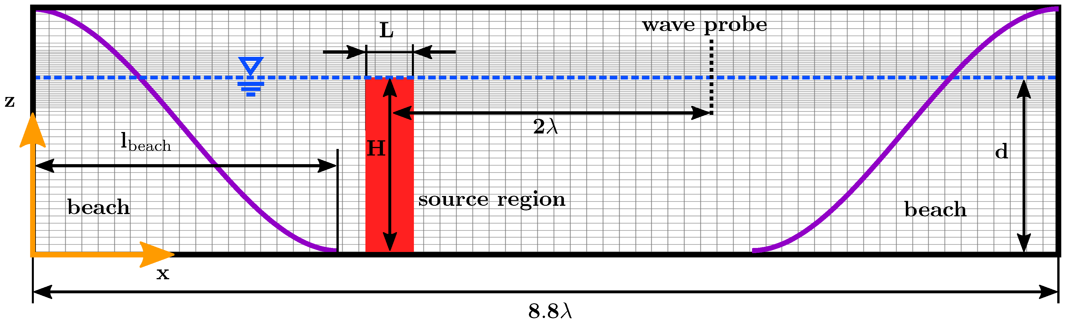
3.4.1. Geometry
The NWT geometry is depicted in Figure 3. The depth of the NWT was set to for the shallow water case, for the intermediate water case and for the deep water case. The target location for the input wave packet was located downwave from the centre of the wavemaker source region. Two absorption beaches were then located at upwave and downwave from the source centre.
3.4.2. Boundary Conditions
The front and back faces of the NWT, lying in the x-z plane, were set to empty, indicating a 2D simulation. The bottom, left and right boundaries were set to a wall. The top boundary was set to atmospheric inlet/outlet condition.
3.4.3. Mesh
The mesh is depicted in Figure 3. The mesh was one cell thick in the y direction, for the implementation of the 2D simulation. Mesh refinement has been employed in the interface region leading to a cell size of eight cells per and 100 cells per wavelength. The spatial discretisation has been chosen based on prior user experience. Furthermore, a grid convergence study has been performed to determine these sizes; based on the case of the wave packet in intermediate water depth. The resulting grid size was consistent with commonly-used discretisations found in the literature [37]. Adjustable time stepping, based on a maximum allowable Courant number of , was used in all simulations.
3.4.4. Calibration of the Numerical Beach
Perić and Abdel-Maksoud [26] recently published a method based on analytical theory to find the ideal magnitude of the damping parameter for monochromatic waves. In the future, it will thus be possible to set the ideal damping parameters prior to each simulation. Herein, a parameter study is performed to investigate the absorption performance for the wave packet. Three different pairs of and were tested for the intermediate water case, i.e.: and ; and ; and . The first test, using and , yielded a reflection coefficient of , with reflection evaluated using the method described by Mansard and Funke [38]. Increasing to resulted in a reflection coefficient of ; using and reduced the reflection coefficient significantly to . The latter beach configuration was then used in all subsequent cases. While even the first configuration, with a resulting reflection coefficient of , was better than for example the experimental facilities described in [27] and many numerical methods, it highlights the flexibility of the approach. Larger beaches will invariably come with a greater computational cost, but for cases where very low reflection over a larger frequency range is required, they seem the only viable method. Figure 3 includes the trajectory of the increasing damping parameter, as used in the simulations.
3.5. Source Region Shape and Position
To investigate the influence of the size and location of the source region, 120 multi-frequency wave packet experiments were run, for 90 intermediate depth cases and 30 deep water cases, with varying source region layouts. For the intermediate water cases, simulations were run with the source region progressively centred at a third, a half, and two thirds of the water depth. For deep water cases, the centre of the source region was located at a depth of , or half the water depth. For each different source centre location, 30 experiments were run with varying the source length region, L, of and varying the height of the source region, H, of and . For brevity, the parametric study on the source region size and location has only been performed for the deep and intermediate water depth case. Since the results were delivered in a parametrised form, as functions of the wave characteristics, the optimal setting found for the deep and intermediate water depth case can directly be applied to the shallow water case.
The performance of the various source region layouts was evaluated as the MSE between the target surface elevation, and the achieved result, :
where K is the total number of time steps in the simulation.
4. Results and Discussion
In this section, the case study results are presented and discussed. First, an example result from a single experiment (deep water case with a source height of and a source length of ) is presented in Section 4.1. The complete set of the results from all the deep, intermediate and shallow water experiments is summarised in Section 4.2, Section 4.3 and Section 4.4, respectively. Application of the simplified calibration method for regular waves is discussed in Section 4.5.
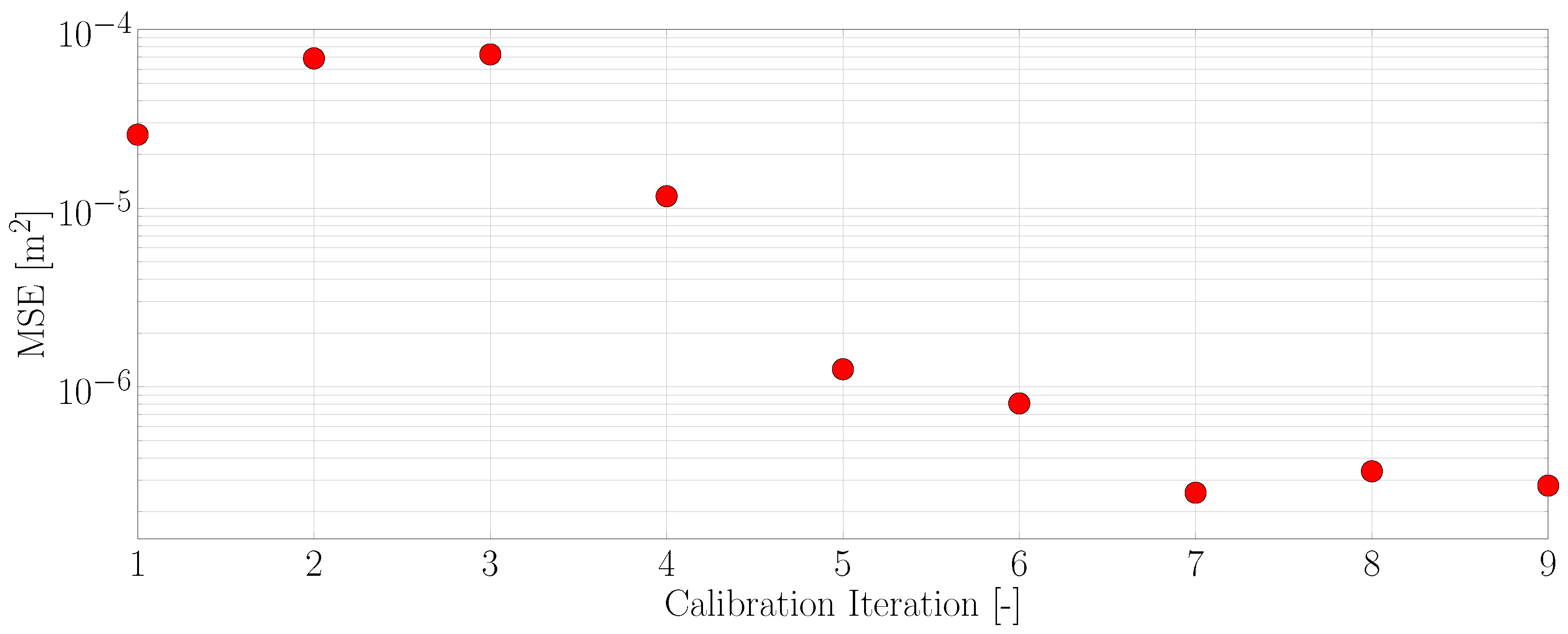
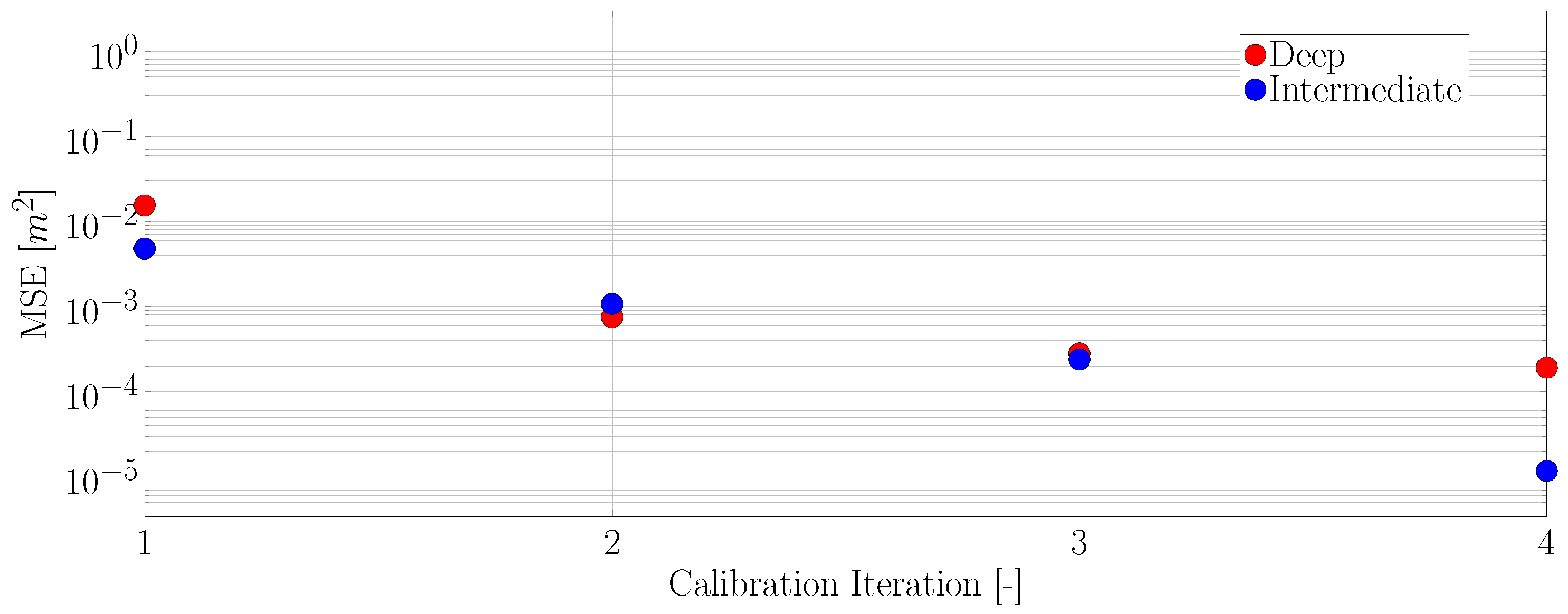
4.1. Example Result
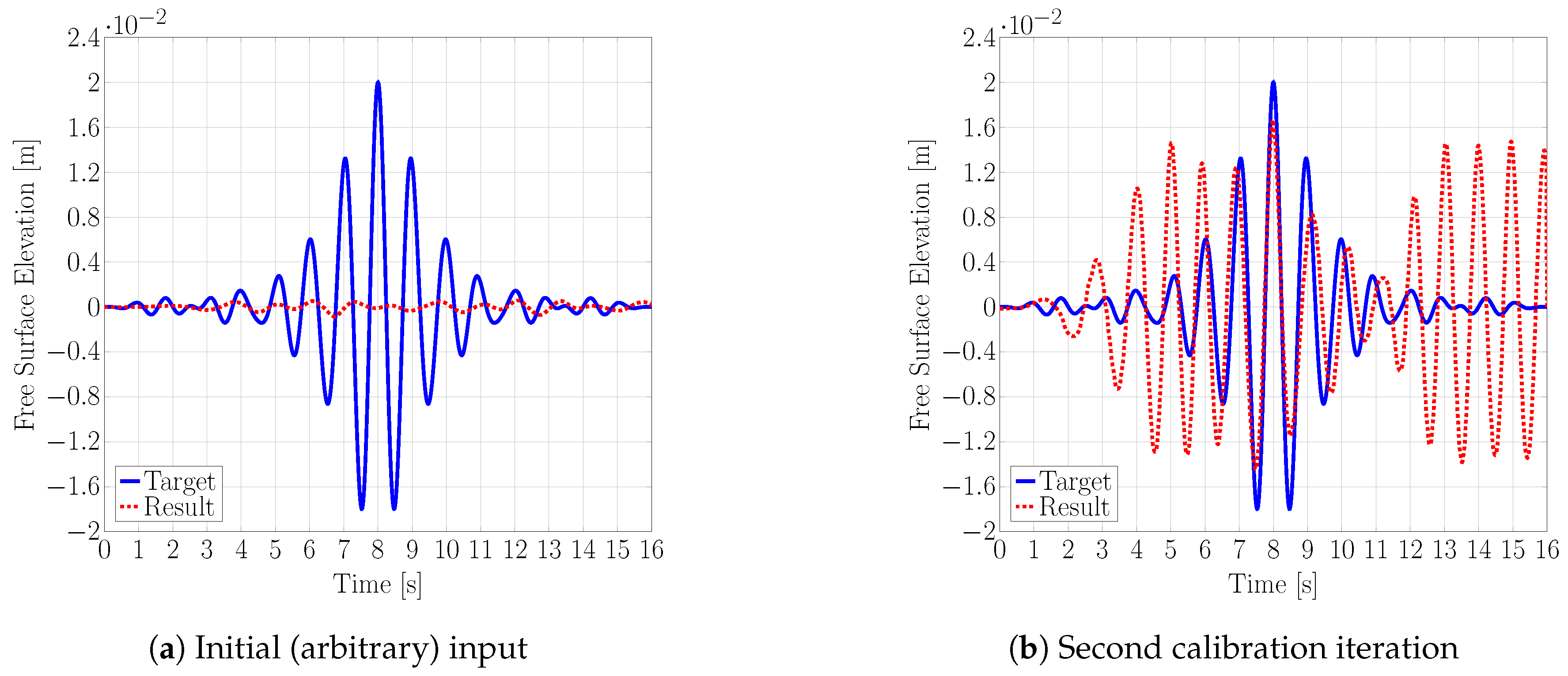
Figure 4 displays an example of the typical decrease in MSE for increasing calibration iterations during an experiment. Note that the evolution is non-monotonic, which is explained by Figure 5, showing the corresponding surface elevation time traces from a selection of these calibration iterations. The first iteration was initialised with random input of small amplitude, and the resulting surface elevation was almost zero, while the MSE of was large. Obviously, convergence could be improved by choosing better initial values, but even for random noise as start values, this behaviour has been observed as typical for all cases. The second iteration yielded several waves with similar amplitude and frequency to the target wave packet, but out of phase, and the resulting MSE almost doubled. The fourth and fifth iterations decreased the MSE by orders of magnitude to and . The main peak of the wave packet was now already correctly resolved, and most of the error stemmed from some small high frequency waves after 11 . Further iterations decreased the MSE to about , and agreement was now further improved for the small ripples after 11 . For all the results presented Section 4.2, Section 4.3 and Section 4.4, nine calibration iterations were used.
4.2. Wave Packet: Deep Water Waves
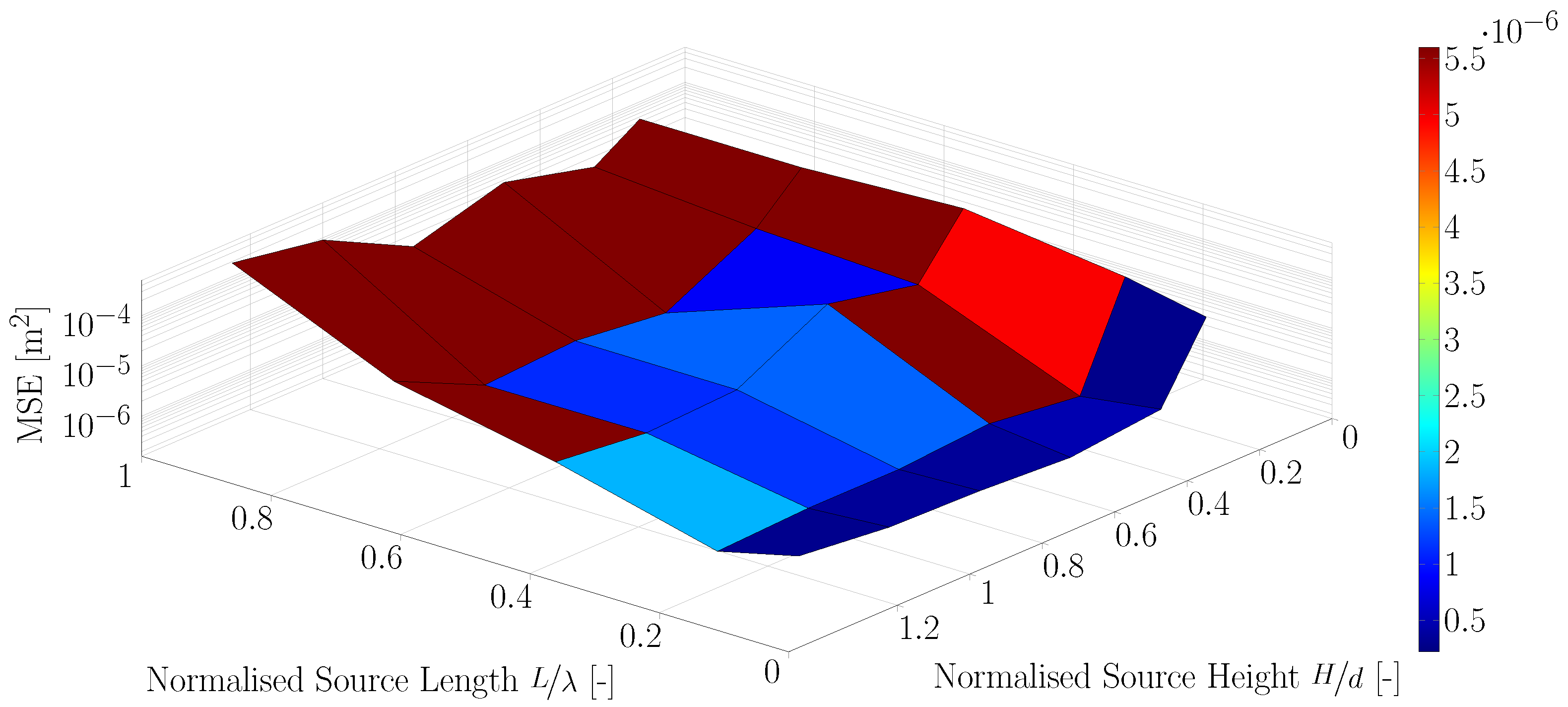
Deep water waves only affect the water column up to a depth of half a wavelength; it thus seems more appropriate to base the vertical position of the source region on that parameter. Test cases were run for varying source heights and lengths, with the source centre position fixed at .
Figure 6 shows the results from the deep water experiments; data are also provided in Table A1. The minimum error was for a source length of and a height of -times the water depth. A wide range of source heights yielded correct results; only for small values of source heights, where the source region did not reach the surface, did the error increase significantly.
4.3. Wave Packet: Intermediate Water Waves
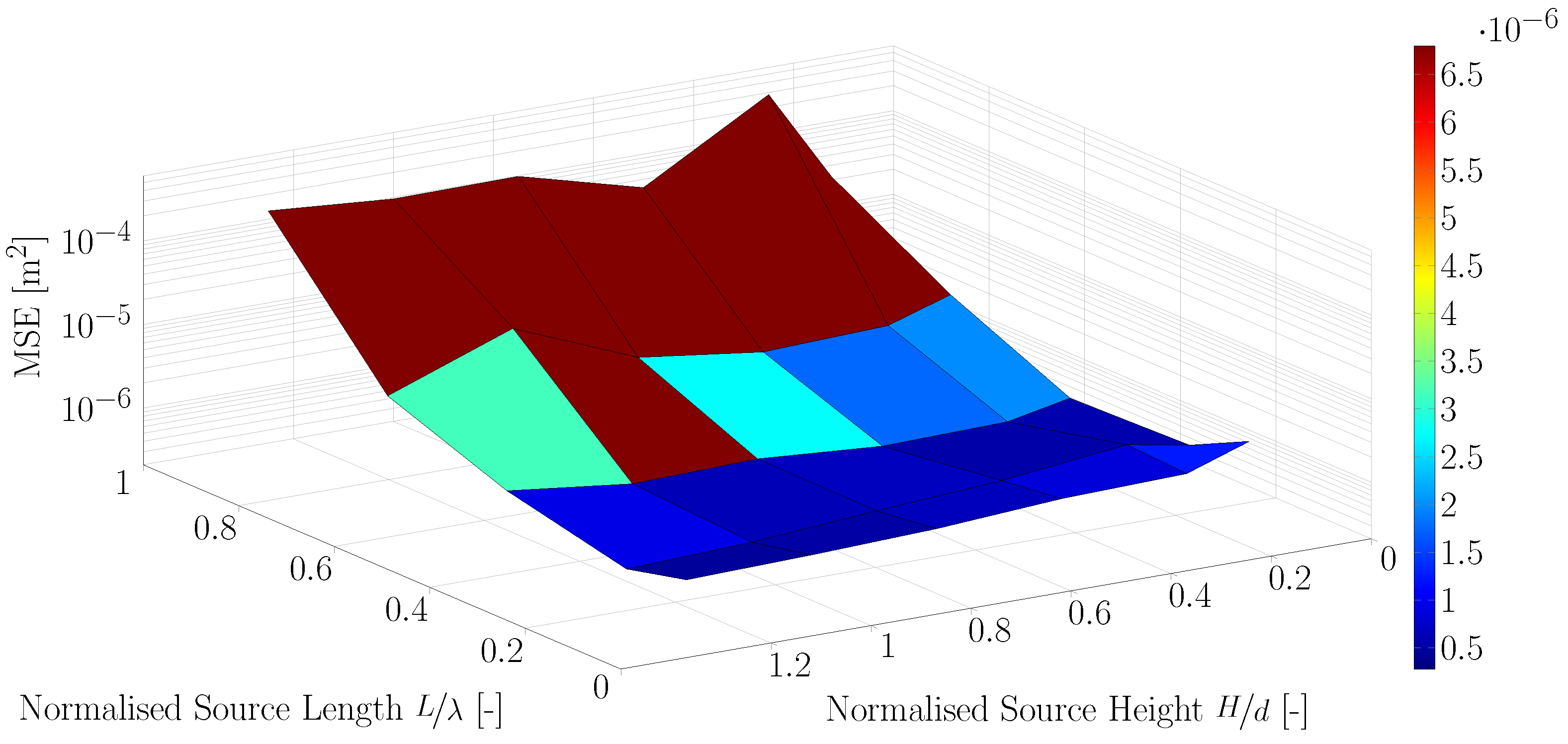
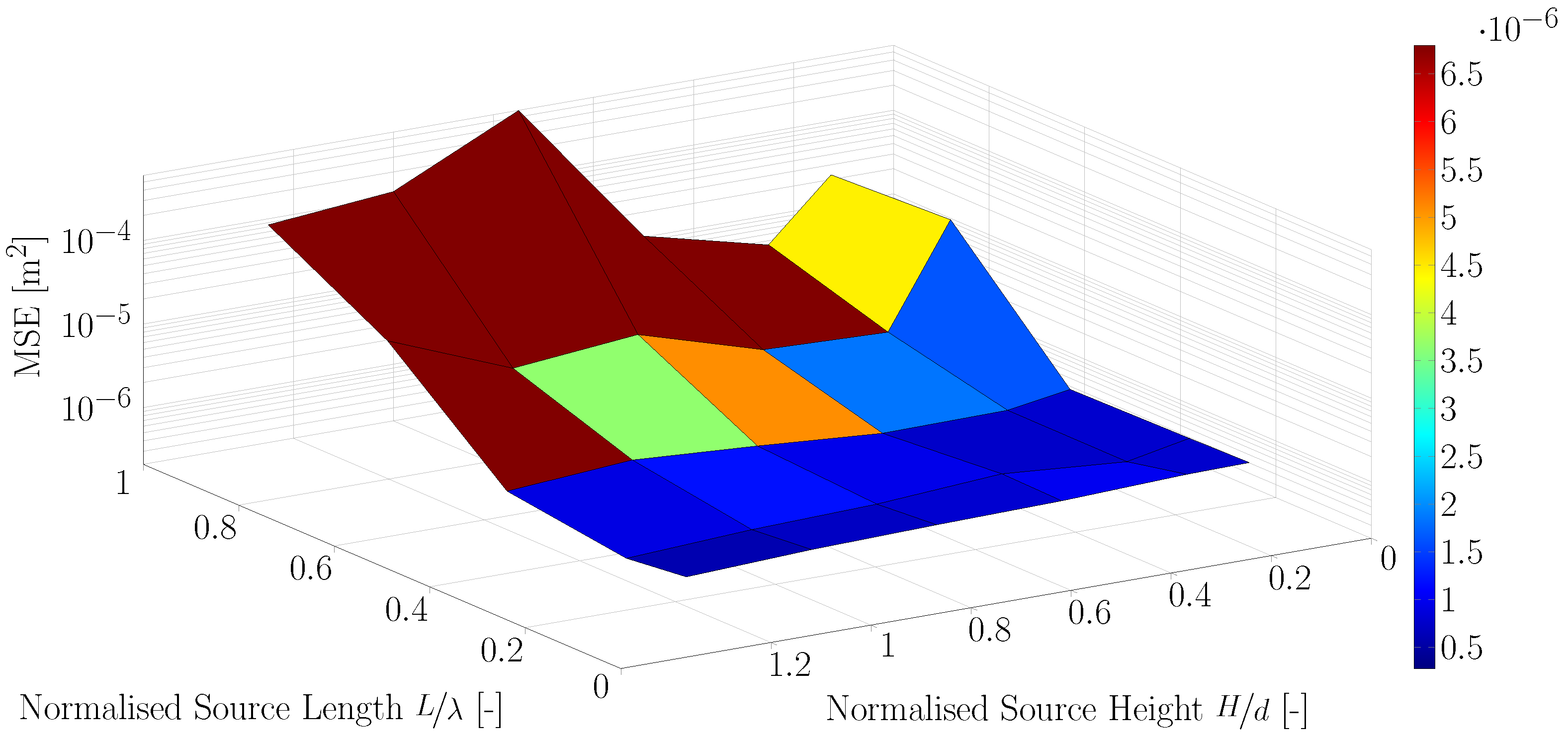
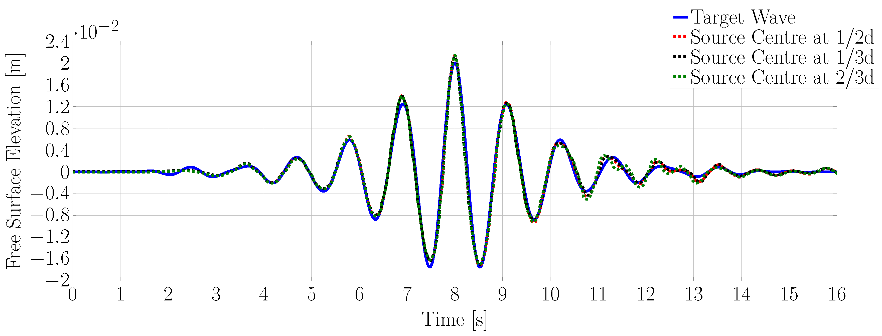
The results from the intermediate water experiments are summarised in Figure 7, Figure 8 and Figure 9 and also in tabular form in Table A2, Table A3 and Table A4. Simulations were run with the centre of the source region at one third, one half and two thirds of the water depth, respectively. The results showed that decreasing the length of the source region, from to or less, reduced the MSE by over two orders of magnitude. In contrast, the height of the source region was seen to have a much smaller influence on the wavemaker performance, with the best results obtained when the source region spanned over the entire water depth. Overall, the smallest MSE occurred for the experiment with the source region centred at half the water depth, the source length of and a source height of -times the water depth.
Figure 10 shows the target wave time series and the results of the experiments that produced the best results for the three different source centre depths. Variations between simulations were minimal. The centre of the wave packet was very well reproduced around its peak and the surrounding crests and troughs, with the main discrepancies occurring at the beginning and the end of the wave packet, with the CFD simulations presenting small amplitude ripples when the target wave was already reaching still water conditions.
4.4. Wave Packet: Shallow Water Waves
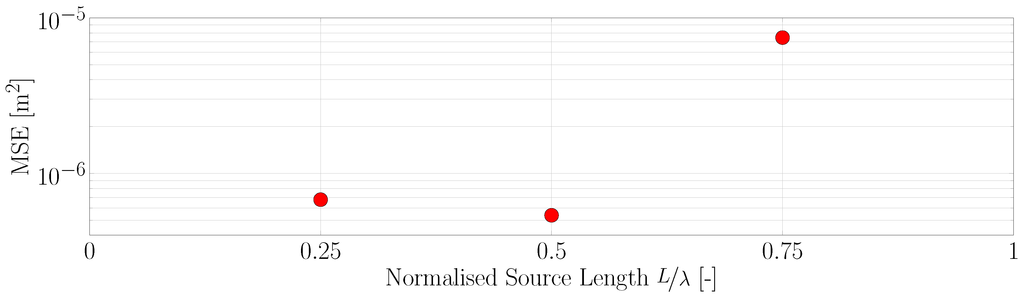
For the shallow water wave experiment, the source region stretched over the whole water column and only different lengths were tested. This seems appropriate considering that depth-independent velocity profiles are a defining feature of shallow water waves. The length of the source was set to , and . Figure 11 shows the resulting MSE values for the three source region lengths, data are also presented in Table A5. The best results were obtained with a length of with an MSE of m. A source length of still yielded good results with an MSE of m. These values are of a similar order of magnitude as the intermediate and deep water cases discussed above. For a source region of , the error increased by an order of magnitude to m.
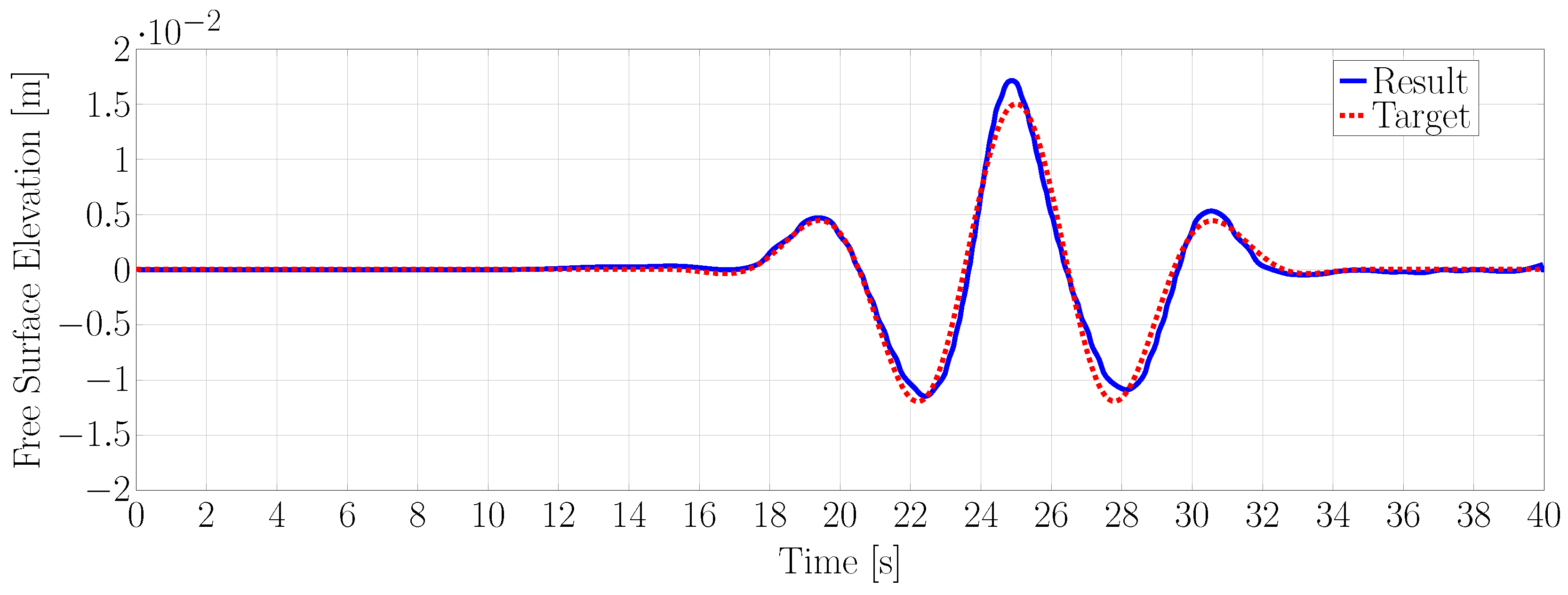
Figure 12 shows the target and resulting surface elevation time traces after nine calibration iterations for the overall best setting, that is a source length of .
4.5. Regular Waves
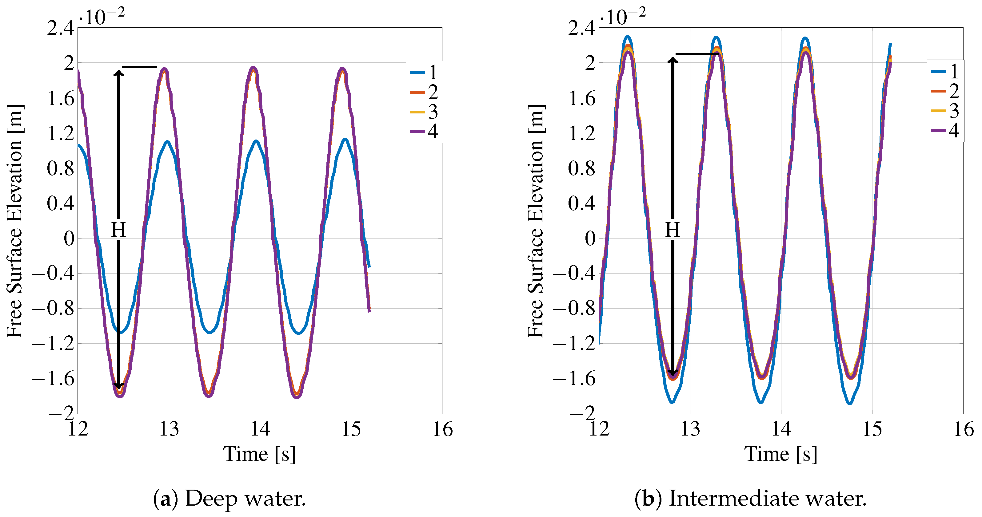
Figure 13 shows the surface elevation during the first four calibration steps for deep and shallow water waves. In both cases, the results converged rapidly; after the second iteration, the results were almost identical for subsequent runs. Figure 14 shows the absolute difference between target wave height and the current value. For the second iteration errors were already within the millimetre range and decreased almost another order of magnitude in the third iteration, which can be deemed sufficient for any practical application.
5. Conclusions
A NWM, based on the impulse source method, was implemented in the OpenFOAM framework. In combination with a calibration procedure, complex irregular wave patterns can be recreated in conditions ranging from deep to shallow water using a simple impulse source term acting in the horizontal direction. While the simple formulation of the source term facilitates implementation in the flow solver and reduces computational overheads, the calibration procedure, which is often required in such cases independent of the wavemaker used, ensures that the target wave is created at the desired position and time in the NWT. Furthermore, reflection analysis demonstrates the transparency of the wavemaker region and the ability of the numerical beach to achieve arbitrarily low reflection. In the future, the work of [26] will allow setting the ideal beach parameters without the need to run parameter or calibration studies.
Parameter sensitivity studies, investigating the effect of the shape and position of the wavemaker region, show that correct results can be achieved over a wide range of parameters. A wavemaker region length of less than a quarter of a wavelength is suitable, which is less than recommended in previous work [18], and might enable the use of smaller computational domains.
The vertical position of the centre of the wavemaker has overall little effect in shallow water conditions, and good results were achieved if it was placed at half the water depth. For deep water cases, good results were obtained with the centre of the wavemaker at a quarter of a wavelength below the surface. Even when starting from a poor initial parameter specification, the method was shown to converge to an accurate solution within a few iterations.
For monochromatic or regular waves, a simplified calibration method can be used. Tests showed that the amplitude can typically be found within four iterations.
Although the calibration method is standard in experimental test facilities, it must be expected to become inaccurate in more nonlinear wave conditions. A possible way forward might be the use of neural networks as described by [21].
Author Contributions
The authors contributed as follows: conceptualization, P.S., C.W. and J.D.; methodology, P.S., C.W. and J.D.; software, P.S., C.W. and J.D.; validation, P.S., C.W. and J.D.; formal analysis, P.S., C.W. and J.D.; investigation, P.S., C.W. and J.D.; resources, P.S., C.W.; data curation, P.S., C.W.; writing—original draft preparation, P.S., C.W. and J.D.; writing—review and editing, P.S., C.W., J.D., J.V.R. and T.W.; visualization, C.W.; project administration, J.V.R. and T.W.; funding acquisition, J.V.R. and T.W.
Funding
This work was supported by a research grant from the Department for the Economy Northern Ireland under the U.S.-Ireland R&D partnership program, Grant No. USI 081. Christian Windt’s Ph.D. is funded by Science Foundation Ireland under Grant No. 13/IA/1886. Josh Davidson is supported by the Higher Education Excellence Program of the Ministry of Human Capacities in the frame of Water Science & Disaster Prevention research area of Budapest University of Technology and Economics (BME FIKP-VÍZ).
Conflicts of Interest
The authors declare no conflict of interest. The founding sponsors had no role in the designof the study; in the collection, analyses, or interpretation of data; in the writing of the manuscript, and in thedecision to publish the results.
Appendix A. Source Region Parameters and MSE Values

Table A1.
MSE values for different source heights and lengths, deep water case.
| Height/Length | 1L | 0.75L | 0.5L | 0.25L | 0.125L |
|---|---|---|---|---|---|
| 1.25d | 1.87 | 7.87 | 1.84 | 2.88 | 7.09 |
| 1d | 9.05 | 1.11 | 1.16 | 3.47 | 4.48 |
| 0.75d | 1.13 | 1.41 | 1.41 | 3.46 | 3.99 |
| 0.5d | 3.60 | 8.57 | 1.21 | 4.74 | 3.10 |
| 0.25d | 1.23 | 6.86 | 4.96 | 2.80 | 4.75 |
| 0.125d | 4.53 | 4.59 | 6.66 | 2.72 | 1.32 |
Table A2.
MSE values for different source heights and lengths, intermediate water case. Centre at .
| Height/Length | 1L | 0.75L | 0.5L | 0.25L | 0.125L |
|---|---|---|---|---|---|
| 1.25d | 1.80 | 2.22 | 4.50 | 4.43 | 6.59 |
| 1d | 1.24 | 1.06 | 4.92 | 4.16 | 6.22 |
| 0.75d | 2.01 | 1.46 | 5.03 | 4.36 | 6.64 |
| 0.5d | 1.34 | 1.40 | 4.66 | 6.81 | 8.24 |
| 0.25d | 1.39 | 2.94 | 5.83 | 9.33 | 1.19 |
| 0.125d | 1.67 | 6.89 | 8.06 | 1.38 | 2.82 |
Table A3.
MSE values for different source heights and lengths, intermediate water case. Centre at .
| Height/Length | 1L | 0.75L | 0.5L | 0.25L | 0.125L |
|---|---|---|---|---|---|
| 1.25d | 1.26 | 3.15 | 9.38 | 4.46 | 6.69 |
| 1d | 9.63 | 1.11 | 6.26 | 5.12 | 7.29 |
| 0.75d | 9.85 | 2.75 | 6.84 | 6.67 | 8.26 |
| 0.5d | 3.97 | 1.75 | 5.35 | 8.43 | 1.04 |
| 0.25d | 2.82 | 1.99 | 5.74 | 1.25 | 1.14 |
| 0.125d | 2.21 | 3.45 | 8.16 | 9.14 | 2.05 |
Table A4.
MSE values for different source heights and lengths, intermediate water case. Centre at .
| Height/Length | 1L | 0.75L | 0.5L | 0.25L | 0.125L |
|---|---|---|---|---|---|
| 1.25d | 8.46 | 1.41 | 9.18 | 5.89 | 7.15 |
| 1d | 1.16 | 3.65 | 1.19 | 7.13 | 8.33 |
| 0.75d | 5.96 | 5.08 | 9.64 | 7.92 | 9.07 |
| 0.5d | 1.03 | 1.84 | 7.52 | 1.00 | 9.65 |
| 0.25d | 4.45 | 1.64 | 7.79 | 7.71 | 1.10 |
| 0.125d | 2.27 | 2.69 | 1.03 | 1.09 | 1.13 |
Table A5.
MSE values for different source heights and lengths, shallow water case.
| Height/Length | 0.75L | 0.5L | 0.25L |
|---|---|---|---|
| 1.25d | 7.47 | 5.38 | 6.78 |
References
- Vanneste, D.; Troch, P. 2D numerical simulation of large-scale physical model tests of wave interaction with a rubble-mound breakwater. Coast. Eng. 2015, 103, 22–41. [Google Scholar] [CrossRef]
- Jacobsen, N.G.; Fuhrman, D.R.; Fredsøe, J. A wave generation toolbox for the open-source CFD library: OpenFoam. Int. J. Numer. Methods Fluids 2012, 70, 1073–1088. [Google Scholar] [CrossRef]
- Dimakopoulos, A.; Cuomo, G.; Chandler, I. Optimized generation and absorption for three-dimensional numerical wave and current facilities. J. Waterw. Port Coast. Ocean Eng. 2016, 142. [Google Scholar] [CrossRef]
- Lu, X.; Chandar, D.D.J.; Chen, Y.; Lou, J. An overlapping domain decomposition based near-far field coupling method for wave structure interaction simulations. Coast. Eng. 2017, 126, 37–50. [Google Scholar] [CrossRef]
- Vukčević, V.; Jasak, H.; Malenica, Š. Decomposition model for naval hydrodynamic applications, Part I: Computational method. Ocean Eng. 2016, 121, 37–46. [Google Scholar] [CrossRef]
- Kim, S.H.; Yamashiro, M.; Yoshida, A. A simple two-way coupling method of BEM and VOF model for random wave calculations. Coast. Eng. 2010, 57, 1018–1028. [Google Scholar] [CrossRef]
- Wu, G.; Jand, H.; Kim, J.; Ma, W.; Wu, M.; O’Sullivan, J. Benchmark of CFD Modeling of TLP Free Motion in Extreme Wave Event. In Proceedings of the ASME 2014 33rd International Conference on Ocean, Offshore and Arctic Engineering 2014, San Francisco, CA, USA, 8–13 June 2014; pp. 1–9. [Google Scholar] [CrossRef]
- Troch, P.; De Rouck, J. An active wave generating-absorbing boundary condition for VOF type numerical model. Coast. Eng. 1999, 38, 223–247. [Google Scholar] [CrossRef]
- Anbarsooz, M.; Passandideh-Fard, M.; Moghiman, M. Fully nonlinear viscous wave generation in numerical wave tanks. Ocean Eng. 2013, 59, 73–85. [Google Scholar] [CrossRef]
- Higuera, P.; Lara, J.L.; Losada, I.J. Realistic wave generation and active wave absorption for Navier–Stokes models: Application to OpenFOAM®. Coast. Eng. 2013, 71, 102–118. [Google Scholar] [CrossRef]
- Brorsen, M.; Larsen, J. Source generation of nonlinear gravity waves with the boundary integral equation method. Coast. Eng. 1987, 11, 93–113. [Google Scholar] [CrossRef]
- Perić, R.; Abdel-Maksoud, M. Assessment of uncertainty due to wave reflections in experiments via numerical flow simulations. In Proceedings of the ISOPE 2015—The 25th International Ocean and Polar Engineering Conference, Kona, HI, USA, 21–26 June 2015; pp. 530–537. [Google Scholar]
- Ren, X.; Mizutani, N.; Nakamura, T. Development of a numerical circular wave basin based on the two-phase incompressible flow model. Ocean Eng. 2015, 101, 93–100. [Google Scholar] [CrossRef]
- Saincher, S.; Banerjee, J. Design of a numerical wave tank and wave flume for low steepness waves in deep and intermediate water. In Proceedings of the 5th International Conference on Asian and Pacific Coasts, Chennai, India, 7–10 September 2015; Volume 116, pp. 221–228. [Google Scholar] [CrossRef]
- Ha, T.; Lin, P.; Cho, Y.S. Generation of 3D regular and irregular waves using Navier–Stokes equations model with an internal wave maker. Coast. Eng. 2013, 76, 55–67. [Google Scholar] [CrossRef]
- Hafsia, Z.; Hadj, M.B.; Lamloumi, H.; Maalel, K. Internal inlet for wave generation and absorption treatment. Coast. Eng. 2009, 56, 951–959. [Google Scholar] [CrossRef]
- Kim, G.; Lee, M. On the internal generation of waves: Control volume approach. Ocean Eng. 2011, 38, 1027–1029. [Google Scholar] [CrossRef]
- Choi, J.; Yoon, S.B. Numerical simulations using momentum source wave-maker applied to RANS equation model. Coast. Eng. 2009, 56, 1043–1060. [Google Scholar] [CrossRef]
- Windt, C.; Davidson, J.; Schmitt, P.; Ringwood, J.V. On the assessment of numerical wave makers for CFD simulations. J. Mar. Sci. Eng. 2019, 7, 47. [Google Scholar] [CrossRef]
- Wei, G.; Kirby, J.; Sinha, A. Generation of waves in Boussinesq models using a source function method. Coast. Eng. 1999, 36, 271–299. [Google Scholar] [CrossRef]
- Schmitt, P. Steps Towards a Self Calibrating, Low Reflection Numerical Wave Maker Using Narx Neural Networks. In Proceedings of the VII International Conference on Computational Methods in Marine Engineering, Nantes, France, 15–17 May 2017; p. 6. [Google Scholar]
- McKee, R.; Elsäßer, B.; Schmitt, P. Obtaining reflection coefficients from a single point velocity measurement. J. Mar. Sci. Eng. 2018, 6, 72. [Google Scholar] [CrossRef]
- Vyzikas, T.; Stagonas, D.; Buldakov, E.; Greaves, D. The evolution of free and bound waves during dispersive focusing in a numerical and physical flume. Coast. Eng. 2018, 132, 95–109. [Google Scholar] [CrossRef]
- Perić, R.; Abdel-Maksoud, M. Generation of free-surface waves by localized source terms in the continuity equation. Ocean Eng. 2015, 109, 567–579. [Google Scholar] [CrossRef]
- Schmitt, P.; Elsaesser, B. A Review of Wave Makers for 3D numerical Simulations. In Proceedings of the 6th International Conference on Computational Methods in Marine Engineering, Rome, Italy, 15–17 June 2015; pp. 437–446. [Google Scholar]
- Perić, R.; Abdel-Maksoud, M. Analytical prediction of reflection coefficients for wave absorbing layers in flow simulations of regular free-surface waves. Ocean Eng. 2018, 147, 132–147. [Google Scholar] [CrossRef]
- Masterton, S.; Swan, C. On the accurate and efficient calibration of a 3D wave basin. Ocean Eng. 2008, 35, 763–773. [Google Scholar] [CrossRef]
- Schmitt, P.; Elsaesser, B. On the use of OpenFOAM to model oscillating wave surge converters. Ocean Eng. 2015, 108, 98–104. [Google Scholar] [CrossRef]
- Schmitt, P.; Asmuth, H.; Elsäßer, B. Optimising power take-off of an oscillating wave surge converter using high fidelity numerical simulations. Int. J. Mar. Energy 2016, 16, 196–208. [Google Scholar] [CrossRef]
- Vorhoelter, H.; Will, J.; Schmitt, P.; Puder, D. Wave Loads on Monopile Structures. In STG Jahrbuch; Hansa GmbH & Co. KG: Bremen, Germany, 2018; Volume 111. [Google Scholar]
- Ning, D.; Zang, J.; Liu, S.; Taylor, R.E.; Teng, B.; Taylor, P. Free-surface evolution and wave kinematics for nonlinear uni-directional focused wave groups. Ocean Eng. 2009, 36, 1226–1243. [Google Scholar] [CrossRef]
- O’Boyle, L.; Elsaeßer, B.; Whittaker, T. Methods to enhance the performance of a 3D coastal wave basin. Ocean Eng. 2017, 135, 158–169. [Google Scholar] [CrossRef]
- Wu, Y.L.; Stewart, G.; Chen, Y.; Gullman-Strand, J.; Lv, X.; Kumar, P. A CFD Application of NewWave Theory to Wave-in-Deck Simulation. Int. J. Comput. Methods 2016, 13, 1640014. [Google Scholar] [CrossRef]
- Rusche, H. Computational Fluid Dynamics of Dispersed Two-Phase Flows at High Phase Fractions. Ph.D. Thesis, Imperial College London, London, UK, 2003. [Google Scholar]
- Eaton, J.W.; Bateman, D.; Hauberg, S.; Wehbring, R. GNU Octave Version 4.2.0 Manual: A High-Level Interactive Language for Numerical Computations. 2016. Available online: https://www.gnu.org/software/octave/doc/v4.2.1/ (accessed on 1 November 2018).
- CCP-WSI. CCP-WSI Repository. Available online: tps://www.ccp-wsi.ac.uk/code_repository (accessed on 19 November 2017).
- Windt, C.; Davidson, J.; Ringwood, J. High-fidelity numerical modelling of ocean wave energy systems: A review of CFD-based numerical wave tanks. Renew. Sustain. Energy Rev. 2018, 93, 610–630. [Google Scholar] [CrossRef]
- Mansard, E.; Funke, E. The measurement of incident and reflected spectra using a least square method. In Proceedings of the Conference on Coastal Engineering (ICCE’80), Sydney, Australia, 23–28 March 1980; pp. 154–172. [Google Scholar]
Figure 1.
Schematic of the calibration method.

Figure 2.
Target wave packet for the impulse wave maker to produce in the case study: surface elevation (a,c,e) and spectral density (b,d,f) for the deep (top), intermediate (middle) and shallow water case (bottom).
Figure 2.
Target wave packet for the impulse wave maker to produce in the case study: surface elevation (a,c,e) and spectral density (b,d,f) for the deep (top), intermediate (middle) and shallow water case (bottom).

Figure 3.
Schematic of the NWT including the main dimensions (schematic not at scale). The function of the gradual increase of in the numerical beach is included in purple. The source region is marked in red. The spatial discretisation, with a fine resolution around the free surface interface, is shown in the background. For the shallow water cases, the water depth d is set to for the intermediate water case to and for the deep water case to .

Figure 4.
Example of the decrease in the MSE for increasing calibration iterations.

Figure 5.
Example of the target and resulting surface elevation, at different calibration iterations, for the same case as Figure 4.
Figure 5.
Example of the target and resulting surface elevation, at different calibration iterations, for the same case as Figure 4.

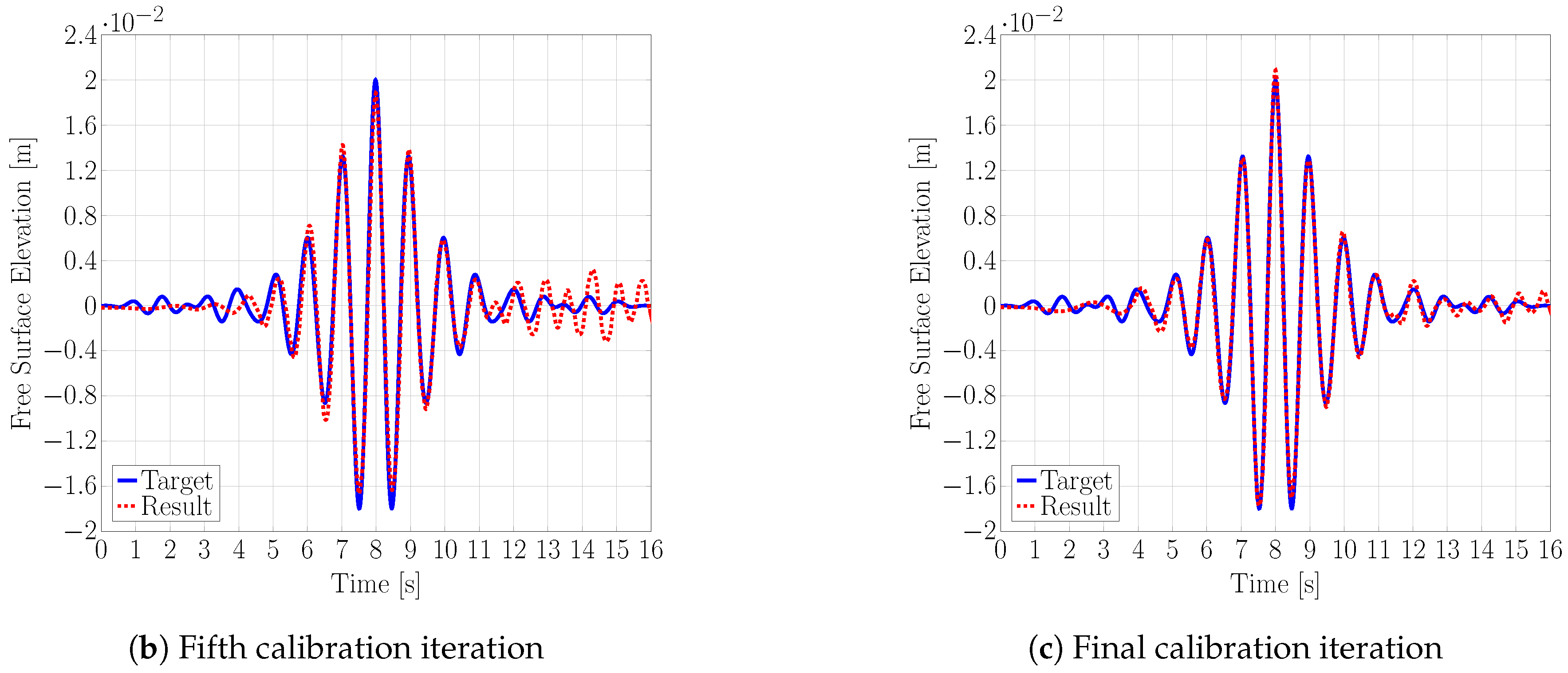
Figure 6.
Deep water case: minimal error ( m) for a source height of and length .

Figure 7.
Intermediate water case. Source centre at : minimal error ( m) for source height of and source length .
Figure 7.
Intermediate water case. Source centre at : minimal error ( m) for source height of and source length .

Figure 8.
Intermediate water case. Source centre at : minimal error ( m) for source height of and source length .
Figure 8.
Intermediate water case. Source centre at : minimal error ( m) for source height of and source length .

Figure 9.
Intermediate water case. Source centre at : minimal error ( m) for source height of and source length .
Figure 9.
Intermediate water case. Source centre at : minimal error ( m) for source height of and source length .

Figure 10.
Surface elevation time series for intermediate water experiments that produced the best results for the three different source centre locations.
Figure 10.
Surface elevation time series for intermediate water experiments that produced the best results for the three different source centre locations.

Figure 11.
MSE for varying source length. Shallow water.

Figure 12.
Target and resulting surface elevation time traces after nine calibration iterations, for the shallow water experiments. Source length .
Figure 12.
Target and resulting surface elevation time traces after nine calibration iterations, for the shallow water experiments. Source length .

Figure 13.
Surface elevation time series for regular waves. Numbers indicate the calibration iteration.
Figure 13.
Surface elevation time series for regular waves. Numbers indicate the calibration iteration.

Figure 14.
Error in wave amplitude versus number of calibration iterations.

Table 1.
Wave characteristics for the wave packet.
| d (m) | (m) | (s) | (m) | (–) | (–) | |
|---|---|---|---|---|---|---|
| Deep water | 0.74 | 0.02 | 0.975 | 1.48 | 0.5 | 3.13 |
| Intermediate water | 0.25 | 0.02 | 1.1 | 1.48 | 0.17 | 1.06 |
| Shallow water | 0.74 | 0.015 | 6.0 | 15.9 | 0.05 | 0.29 |
© 2019 by the authors. Licensee MDPI, Basel, Switzerland. This article is an open access article distributed under the terms and conditions of the Creative Commons Attribution (CC BY) license (http://creativecommons.org/licenses/by/4.0/).
Share and Cite
MDPI and ACS Style
Schmitt, P.; Windt, C.; Davidson, J.; Ringwood, J.V.; Whittaker, T. The Efficient Application of an Impulse Source Wavemaker to CFD Simulations. J. Mar. Sci. Eng. 2019, 7, 71. https://doi.org/10.3390/jmse7030071
AMA Style
Schmitt P, Windt C, Davidson J, Ringwood JV, Whittaker T. The Efficient Application of an Impulse Source Wavemaker to CFD Simulations. Journal of Marine Science and Engineering. 2019; 7(3):71. https://doi.org/10.3390/jmse7030071
Chicago/Turabian StyleSchmitt, Pál, Christian Windt, Josh Davidson, John V. Ringwood, and Trevor Whittaker. 2019. "The Efficient Application of an Impulse Source Wavemaker to CFD Simulations" Journal of Marine Science and Engineering 7, no. 3: 71. https://doi.org/10.3390/jmse7030071
Note that from the first issue of 2016, this journal uses article numbers instead of page numbers. See further details here.