Article

Preliminary Study on the Contribution of External Forces to Ship Behavior

by
Augusto Silva da Silva
1,*,†,
Phelype Haron Oleinik
1,†,
Eduardo de Paula Kirinus
1,†,
Juliana Costi
2,†,
Ricardo Cardoso Guimarães
1,†,
Ana Pavlovic
3,† and
Wiliam Correa Marques
2,†
1
Escola de Engenharia, Universidade Federal do Rio Grande Campus Carreiros, Av. Itália s/n Km 8, Rio Grande 96201-900, Brazil
2
Instituto de Matemática, Estatística e Física, Universidade Federal do Rio Grande Campus Carreiros, Av. Itália s/n Km 8, Rio Grande 96201-900, Brazil
3
Department of Industrial Engineering, University of Bologna, Viale Risorgimento 2, 40136 Bologna, Italy
*
Author to whom correspondence should be addressed.
These authors contributed equally to this work.
J. Mar. Sci. Eng. 2019, 7(3), 72; https://doi.org/10.3390/jmse7030072
Submission received: 15 January 2019 / Revised: 11 February 2019 / Accepted: 20 February 2019 / Published: 20 March 2019
(This article belongs to the Special Issue Engineering Mathematics in Ship Design)

Abstract

:
Computational modeling has become a prominent tool to simulate physical processes for research and development projects. The coastal region of southern Brazil is very susceptible to oil spill accidents. Currently, oil is intensively transported in the region due to the presence of the Rio Grande Harbor, the Transpetro Waterway Terminal (Petrobras) and the Riograndense S/A Oil Refinery. Therefore, simulations under ideal navigation conditions for ships with potentially polluting loads are important because their use can reduce oil spills and toxic compound accidents in the environment. Therefore, the main objective of this work is to present a preliminary study of the contribution of external forces to a ship’s behavior over a simulation period of 5 h. The methodology is based on the development of a numerical model using LaGrangian formalism and the calculus of variations, besides Maneuvering Modeling Group (MMG Model). The external forces considered were the wind acting directly on the ship, waves driven by wind, the rudder, the force acting on the hull, inertial forces, and seawater density. The results indicate that at the beginning of the simulation, the inertial forces were of primary importance for controlling the trajectory of the ship. After 5 h of simulations, the ship had completely changed its trajectory due to forces suffered by the ship, classified according to MMG Model.

1. Introduction

Shipbuilding industry challenges have intensified the development of new operational configurations of high-speed ships for ocean-articulated convoys [1], as well as the phase approach of side discharge arrangement for tankers and fuel-supplying techniques to military vessels. These new operation conditions have produced additional challenges into the hydrodynamics interference on vessel dynamics mostly caused by radiated and diffracted waves between vessels. With that in mind, new resources aiming to better understand the vessel interaction with the ocean are constantly being developed, and with the advances of numerical models, these are, more often than not, being used to assess the operational limits and the effects of the hydrodynamic interference, of ship structures.
The influence of waves and hydrodynamic forces on vessel dynamics have been the subject of many studies over the years. Froude [2] conducted the pioneer study of ship movement, considering the effects of successive waves on ship movement. The study of Michell [3] was the first to take into account the disturbance imposed by a vessel in the flow, and originated the Thin Ship Theory. This theory was further developed and improved by many other authors (e.g., [4,5,6]). More recently, reference [7] presented the Band’s Method, which evaluates the influence of hydrodynamic forces along bands of the vessel.
Then, a research group called Maneuvering Modeling Group (MMG) developed a numerical model to study the movements performed by a vessel when maneuvering. This model is known as MMG Model, and was reported in the Bulletin of Society of Naval Architects of Japan in 1977 [8]. However, the data used in this simulation were not detailed. Subsequently, Ogawa and Kasai [9] and Inoue et al. [10] published studies detailing this study, including equations describing the external forces.
Many simulations based on MMG Model were reproduced and published using different methods to acquire data, and manipulate and interpret results, so the Japan Society of Naval Architects and Ocean Engineers created a research committee to develop studies using a standard method for MMG Model. Yasukawa and Yoshimura [8] made a introduction of this standard method, splitting it in four essential elements and used a tanker to validate the study, concluding that the method used could represent the movements realized by a vessel and would be useful to predict these movements at full scale.
This study is about numerical simulations that use a specific model called SHIPMOVE. This numerical model uses variational theory and LaGrangian mechanics to calculate the trajectory of the ship and its angular movements.
SHIPMOVE does not use the theories already cited, but it incorporates in its basic equations the MMG Model equations. The SHIPMOVE basic equations describe the ship’s position considering the kinetic and potential energy. Also, this model considers additional mass and drag forces due to friction and generation of waves.
Over the years, several methods have been developed to investigate the behavior of ships under the influence of external forces in seakeeping or maneuvering. Thus, the objective of this study is to present the first results obtained using a numerical model that was developed to study ship dynamics under the influence of external environmental forcing.

2. Material and Methods

To perform this study, numerical simulations were performed using the hydrodynamic model TELEMAC-3D, the wind-driven waves model TOMAWAC, both part of the open TELEMAC-MASCARET suite1 and SHIPMOVE. The latter was developed by the Laboratório de Análise Numérica e Sistemas Dinâmicos2. The simulations were realized through the coupling of TELEMAC-3D+TOMAWAC feeding SHIPMOVE with hydrodynamic and wave data.
The SHIPMOVE model describes ship movement in the time domain using variational theory and LaGrangian mechanics. A detailed description of the first version of the model that does not include the MMG formulation, is provided in [11].

2.1. TELEMAC-3D

The open TELEMAC-MASCARET system is formed by a set of modules, operating in two or three dimensions, which can be used for different case studies such as hydrodynamics, sediment transport, dredging processes, waves driven by wind, pollutants, or oil spills, renewable energy, and more.
TELEMAC-3D is part of the open TELEMAC-MASCARET system, and it is responsible for the hydrodynamics of this study. It solves the Navier-Stokes equations [12] considering hydrostatic pressure and Boussinesq approximations [13]. Also, it solves the free surface variations in function of time. To solve the advection and diffusion hydrodynamic equations, the model uses the finite element techniques meanwhile for vertical discretization, TELEMAC uses sigma levels to segment the ocean from the surface to the bottom boundaries [13].
Some of the approximations used in TELEMAC include the simplification of the vertical velocity w, since it presents a small scale when compared with the u and v velocities. In this way, the vertical diffusive term in addition to other vertical terms are simplified from the calculations. However, terms that consider hydrostatic pressure variations and gravity acceleration are maintained in the vertical equation of momentum, so the pressure at any point in the ocean depends on atmospheric pressure above the water column weight over this point. Due to Boussinesq approximation ( Δ ρ supposedly small when compared to a reference), it is possible to define the influence of the seawater state equation [14], because this equation relates specific mass of the fluid with the tracer concentration in this water.
Substances or properties that are present in water, such as temperature, salinity, and suspended sediments, are defined as scalar quantities, and can be active (when they interact with the hydrodynamic), or passive (when they do not interact). The advection processes, governed by sea current and wind, and diffusion, governed by turbulent processes from sources and sinks, control the temporal evolution of these scalar quantities.
In this way, TELEMAC-3D is used in the system to provide information about the hydrodynamics, mostly the current velocities, which will later feed the SHIPMOVE module.

2.2. TOMAWAC

To add the wave field into the vessel simulations, TOMAWAC (TELEMAC-Based Operational Model Addressing Wave Action Computation) module was used to perform the calculations. TOMAWAC is a third-generation wave model and part of the open TELEMAC-MASCARET suite.
TOMAWAC is a spectral model and generates waves through the wind, based on the wave action density conservation equation [15]. TOMAWAC considers most physical processes involved in wave generation, such as shoaling, whitecapping, dissipation through bottom friction, non-linear interactions, and depth-induced refraction; however, it does not consider wave diffraction and reflection [15].
To solve the equation cited above, TOMAWAC splits the direction wave spectra in a finite number of propagation frequencies and directions and solve these equations for all components without parametrization to any direction, spectral energy or wave action. Every wave spectrum component evolves in time according the modeled system.
The function of the TOMAWAC module in this study is to feed the SHIPMOVE model with ocean wave properties, such as the significant wave height and the peak direction of the waves.

2.2.1. Maneuvering Modeling Group (MMG Model)

MMG Model is one of the various numerical methods used to solve simulations involving ship maneuverability, and was used in this study. This model applies to ships, characteristics, and consequences from the involved forces at hull, propeller, and rudder, beyond the interaction between them.
The main objective of this model is to simplify the external forces application on vessel routes studies; however, there are some methods used on simulations that harm those studies, since one method used in some cases may be not appropriated to another one.
In this paper, 6 DOF are considered, differentiating from [16], where only surge, sway, and yaw movements were considered.
According to Maimun et al. [17], the ships have their movements significantly affected when sailing in shallow water, such as canals, because the hydrodynamic interaction between the ship and the bank located on laterals or bottom restrict the movements and develop other forces. Here, the bank effect will not be considered since the vessel travels to places where the relation between draft/depth does not produce this effect.
In this way, the force equations produced by the MMG Model, for both, x and y axis follows (Equations (1) and (2)):
X A + X W + X R + X H = F x e
Y A + Y W + Y R + Y H = F y e
where the subscriptions A, W, R, H represent wind, wave, rudder, and hull, respectively.

2.2.2. Wind forces

For the wind forces that act on the vessel Equation (3) are presented. These equations are used by the SHIPMOVE module to simulate the action of the wind at the ship:
X A = 1 2 ρ A V A 2 A T C X A ( θ A )
Y A = 1 2 ρ A V A 2 A L C Y A ( θ A )
where ρ A is the density of air, V A is the wind velocity, A T and A L are lateral projected area and frontal projected area, respectively. C X A and C Y A are coefficients based on the relative wind direction, estimated by Andersen [18].

2.2.3. Wave Forces

For the wave effects acting on the vessel, Equation (4) are presented. The wave properties are first calculated trough TOMAWAC and with its output, the SHIPMOVE model is then capable of simulating the wave forces that are acting on the ship:
X W = ρ g h 2 B 2 / L C X W ¯
Y W = ρ g h 2 B 2 / L C Y W ¯
where ρ is the density of seawater, g is the acceleration of gravity, B represent ship’s breadth, h is the significant wave height, C X W ¯ and C Y W ¯ are coefficients calculated by the Research Initiative on Oceangoing Ships (RIOS) [19].

2.2.4. Rudder Forces

SHIPMOVE also takes into account the forces provoked by the rudder of the vessel (Equation (5)):
X R = ( 1 t R ) F N s i n δ
Y R = ( 1 + a H ) F N c o s δ
where F N is the rudder normal force, δ is the rudder angle, t R and a H represent the steering thrust deduction factor and rudder force increase factor, respectively.
The rudder normal force can be expressed as Equation (6):
F N = 1 2 ρ 6.13 λ λ + 2.25 A d U 2 s i n α R
where ρ is the density of water, λ is the rudder aspect ratio, U R was approximated to the ship’s velocity, A d denotes rudder area and α R is the relative inflow angle to rudder [20].

2.2.5. Forces Acting on the Hull

The hydrodynamic forces on the ship’s hull and used in the SHIPMOVE model are given as Equation (7):
X H = 1 2 ρ L 2 U 2 X H ( v , r ) R ( u )
Y H = 1 2 ρ L 2 U 2 Y H ( v , r )
where r denotes non-dimensionalized yaw rate by r ( L / U ) , and v represent non-dimensionalized lateral velocity v / U . X H and Y H are polynomial functions of v and r . R ( u ) is the ship resistance, which depends on residuary resistance coefficient, frictional resistance coefficient and the form factor [20].

2.3. Numerical Experiments

To study the influence of external forces acting on the ship, five simulations were performed. Each simulation represents a different external force described by the MMG Model: hull, rudder, wave and wind, and the fifth simulation was a case where the ship navigated without any external forces. These cases were performed seeking for differences between the trajectories of the ship in each case and how the forces affect the performance of the ship.
All cases were performed with the same initial conditions and the same simulation day: 5 April 2012. The climate characteristics of this day were chosen because, from meteorological data sets3, it was noticed that the sea conditions, currents, and waves were at a low strength, allowing the ship to perform its movements without any extreme forces, avoiding peaks. The vessel navigated five hours in the open sea direction, departing from the south Brazilian coast.

2.4. Initial and Boundary Conditions

The definitions of initial and boundary conditions are essential to the initialization of the numerical model. They specify the physical characteristics of the vessel used in the simulation and the environmental conditions surrounding the ship (water temperature, salinity, water density, significant wave height, velocity, and acceleration of the waves).
The physic characteristics of the ship are shown in Table 1.
The hydrodynamic simulation required the definition of boundary and initial conditions for the TELEMAC3D, which were obtained from the Hybrid Coordinate Ocean Model (HYCOM4). HYCOM data provides water temperature and salinity and current intensity with horizontal resolution of 0.083°; such data is interpolated to the ocean boundary conditions.
At the free surface, the atmospheric boundary conditions (wind, air temperature, and pressure) were obtained from NCEP/NCAR Reanalisys5, from NOAA, with spatial resolution of 1.875° and temporal resolution of 6 h.
To initialize the wave model, TOMAWAC, WAVEWATCH III6 dataset was used to force the ocean boundaries (spatial resolution of 30 min and temporal of 3 h). Wind data from NCEP/NCAR Reanalisys7 with spatial resolution of 1.875° and temporal resolution of 6 hours were also used to force the superficial conditions of the wave model.
This study was carried out using data from the period between January and December of 2012. In order to represent the spatial domain, a mesh with 205.617 nodes (Figure 1) was used, with 1.5 km between nodes near the coast, and 8 km, approximately, in ocean boundaries.

3. Calibration and Validation

To validate the hydrodynamic and wave models a simulation comprising the year of 2013 was performed and compared against observed buoy data.
A validation comparison was performed throughout a comparison of time series, the modeled and observed, and applied a set of performance skills and statistical metrics to validate TOMAWAC ( H m o and T p ) and TELEMAC-3d (intensity of current velocity) results. The comparison was done with the time series measured by the wave buoys from PNBOIA8 (Programa Nacional de Boias) which is a Brazilian project to collect oceanographic and meteorological data along the Brazilian coast. The data from PNBOIA were obtained on the coast of Santa Catarina (28.8333° S, 47.6000° W, 500 m depth) (Figure 1).
Despite the small number of observed data (5 months) available for 2013, the time series comparison between model and buoy data (Figure 2) indicates a good representation of the model results, when compared to the buoy data tendency. Nonetheless, visual comparison cannot be used on its own to define the accuracy of the model.
The usage of statistical metrics and well-known performance skills can quantify this comparison for better understanding the tendencies observed [21,22,23,24,25]. The desirable results for these statistical metrics are values closer to 0 (for RMSE, MAE, MSE, Bias, and SI), while others indicate better agreement between model and buoy with values closer to 1 (IC, SS, R 2 ).
At Table 2, H m o shows low RMSE values (near to 0.6 m), this tendency is enforced by low MAE values with 0.43. These values are lower than those found in the literature [23,26]. The Willmot Concordance Index (IC) [21] represents the ability of the model to reproduce the observations, resulting in 0.70, the accordance of the model data presents good confidence.
Despite the differences presented (Table 2), other wave statistics ( R 2 , Bias, SI and SS) were also applied to the analysis [22,27,28] to better validate the accuracy of the model. Khandekar [27] performed several model verifications with statistical methods, concluding that most models with SI lower than 35% are considered able to predict the studied environment; for instance, all SI comparisons (Table 2) show competence [28].
Standard deviation and mean values are within the range of acceptance, with bias close to zero indicating excellent agreement between predicted and observed data. A slight overestimation of the model data over the buoy is observed since SS values are higher than 1. The Pierson correlation coefficient (R) remains around 0.70, which is an acceptable result, according to Lalbeharry [23].
Telemac-3d ability to predict the buoy data was evaluated for the intensity of velocity (Table 2). RMSE (MAE) of 0.16 m· s 1 (0.13 m· s 1 ) presented low values in this comparison resulting in good agreement, in addition to an IC of 0.86. The MSE presented values closer to zero in all cases, indicating good agreement between model and buoy.
In this section a validation has been discussed in terms of current and wave parameters, whereas the hydrodynamic model Telemac-3d and wave model TOMAWAC were able to show good reproducibility of results behalf the buoy data and also being able to maintain the patterns and tendencies observed.

4. Results and Discussions

To study the influence of each force involved in the MMG Model methodology, five simulations were performed with the forces applied separately. The vessel had an initial velocity of 9.72 knots on the x axis, and −9.72 knots on the y axis, resulting in 13.7 knots approximately (the resulting vector). This energy was dissipated over the time according to the intensity of each force of the MMG Model and the dissipative forces.
The forces applied in the model are not necessarily dissipative forces only—they can be viscous forces, sometimes dissipating the ship energy, sometimes “helping” the ship to perform its movements. It depends on the relative direction between the forces and the ship.
Figure 3 shows the results of 5 h of simulation on 5 April 2012. This figure shows the routes performed by the ship with each influence applied separately, in all cases with the same initial conditions. Wave height is shown in the color bar. White vectors represent the wave direction while the black vectors represent wind direction.
To compare the simulated cases and see the differences between the ship with and without external forces, a simulation where no forces were involved and the ship had only the initial velocity condition was performed; in this way, the vessel dissipation of the energy only occurred trough the viscous and frictional forces acting as drag forces, as well as the dissipation trough the additional mass of the ship.
Chen et al. [19] showed the wind influence on a vessel’s trajectory, when the vessel trajectory was deflected to North due to the influence of South acting wind. In the present study, it was possible to confirm that wind factor exerts a major role determining the trajectory distance and direction, while ocean currents induce more variations on rotational angles of the ship movements.
When the wind influence was simulated by the SHIPMOVE, it was possible to notice affinity to the results presented by [19]. On the simulation day, the wind conditions had major incidence direction of east. In this way, it was expected that the ship should deflect to starboard, and start to change its route direction South. From Figure 3 it is possible to notice that the ship did deflect to starboard corroborating with the previously studies, and demonstrating the accuracy of the SHIPMOVE.
Also, in Chen et al. [19], the effects of incident waves striking the lateral of vessels were studied. The authors conclude that waves focusing on the lateral of the ships have the strength to drive the vessels to the wave direction. For example, if the waves come from the South and collide on the lateral of a vessel, it will deflect the vessel trajectory a few degrees North.
Once again the present study demonstrated good agreement with the literature. For the case study, the waves of the simulated day were traveling North, with significant wave height varying from 2.5 m to 1.5 m close to where the vessel trajectory was calculated. With these conditions, the wave action was capable of deflecting the vessel trajectory port and deflect the trajectory that firstly started South-east to East and tendency to go North-east.
When the rudder force is analyzed trough the SHIPMOVE model it is possible to notice the proportionality of the force compared to the ship velocity; therefore, the force tends to reduce over time along with velocity. In the beginning of the simulation, the force is capable of making the ship change its direction to the North-east; however it is not strong enough to make the ship dissipate its initial energy totally; then, the vessel obtained a large trajectory, been the forces in x and y axis positives, in this case, first quadrant of a Cartesian grid.
The case in which the ship suffers hull force is similar to the rudder force case, but in the hull case the force is great enough to make the ship dissipate its initial velocity, and that is the reason the vessel trajectory is so small. In the first moment, the force is so strong that it can almost stop the ship, but when its velocity becomes small, the forces follow the velocity decay, allowing it to move, even with a small velocity. This is why the ship does not stand still over the 5 h of simulation.
The total distance performed by the ship in all cases can be discovered by calculating the resulting distance; Figure 4 shows the distance in each axis of the translational movements of the vessel.
In the case of only wind force acting on the ship, it covered approximately 65 km on the x axis and 90 km on the y axis, totalizing 112 km. With only the hull force, 21 km on x axis and 4 km on y axis totalizing 22 km. The study case only with wave forces was when the ship had his greater trajectory on x axis, 132 km, and 48 km on the y axis, totalizing 140 km. The ship navigated 117 km in the rudder case (110 km on x and 40 km on y). When the ship was simulated only with initial velocity, without any of the forces applied, it navigated 100 km, approximately (79 km on x and 61 km on y). Figure 4 also shows the ship’s linear movements on z axis (heave movement), which has much smaller magnitude in all cases.
The timeline of ship’s velocity in each case can be seen in Figure 5.
To better understand the movements performed by the ship, we studied the velocity timeline of the ship over the 5 h of simulation for each case.
When the ship suffered only the wind forces, its velocity remained almost constant, reaching 10.5 knots near to the second hour of simulation, and then it raised to 12.5 knots approximately.
The ship had the greater velocity in the wave forces case, reaching 22.5 knots in the last hour of simulation, but it had a minimum (12.5 knots) between the second and third hour of simulation. The increase of the velocity can be attributed to the wave direction. In Figure 3, the wave starts to push the ship North.
In the rudder case, the ship had a peak near the beginning of the simulation, reaching more than 15 knots, but it starts to decrease after the first hour of simulation, and finishes with less than 10 knots. The hull case was the slowest case of them all. The ship began with 13.7 knots and then started to slow down from the beginning because the velocity depends on the force. The ship, after the first half hour of simulation, stabilized near to 2.5 knots and finished with this speed.
To finish, the case where the ship navigated only with the initial velocity dissipating its energy due to dissipative forces, had an initial velocity of 13.7 knots and, almost linearly, decreases to 8 knots. This is acceptable due to the fact that no external forces are involved, so the dissipative forces remain almost the same during all 5 h of simulation, since the ship and fluid properties did not change during the simulation.
Also, the angular movements of the vessel were studied in for every case, as shown in Figure 6.
Looking at the roll movement, the vessel had the greater oscillation in the hull case (−0.225°), it can be attributed to the fact that the vessel had smaller speed, so the hydrodynamic forces could act more intensely.
On the other hand, in the wind case, the ship remained near to 0°, corroborating the study of Chen et al. [19] that said the wind has a smaller contribution on angular movements.
When the ship navigated without any external forces, its movement was a little larger when associated with the wind case, transcending −0.1°, but its variation from 0° to 0.125° was almost linear.
In the rudder case, the ship oscillated around −0.2°, with a peak (−0.22°) around the first hour of simulation. After that it stabilized on −0.2°.
The roll movement on the wave case was the case where the ship had the greatest instability, varying from 0° to almost −0.2°, and between the third and fourth hours of simulation the ship presented a movement of −0.075°.
Almost all cases were positive in the pitch movement, with the wave case as the largest one and the case where the ship had its greater variations, the same occurred in the roll movement, due to the high speed. It reached 0.25°.
Right below was the rudder case with 0.24° as a peak in the first hour. After this, it stabilized in 0.225° until the end. In the hull case the ship did not oscillate after the first hour, remaining on 0.16°. In the case without any external forces the ship had not transcended 0.1°, been almost linearly variation.
The only case in which this movement was negative was in the wind case, remaining near to 0° during the 5 h of simulation, showing again the fact that the wind has no major influence under angular movements.
In the yaw movement, the hull case was the case that the ship had the largest value, reaching −0.24°, but it had no oscillations during its simulation after the first hour, showing stability. The rudder case was the second largest value, remaining in −0.21° with a little variation between the first and the last hour of simulation.
When the ship navigated suffering no external forces, it had the second largest instability (0° to −0.125°), increasing almost linearly during its simulation. In the wave case, the ship had larger oscillations, varying from 0° to −0.07°, and then returns near to −0.05°. After the fourth hour of simulation, the ship performed yaw movements from −0.06° to −0.15° in the end. Again, the wind case was the case with fewer values related to angular movements. In general, all cases the ship had behaved similarly in roll and yaw movements, coincidentally.
When it is stated that there were more variations or instability, it means the ship had more variations during the 5 h of simulation—it does not mean the difference between the initial and the final value. It can be understood that in the cases where the hull and the rudder were studied, the ship reaches some stability near to the first hour and in the other cases, the angular movements vary during all simulation periods.
The behavior of the ship observed in all cases disagrees with the results reported by similar studies (Cha and Wan [29], Chuang and Steen [30], Bennett et al. [31], Ozdemir and Barlas [32]). Cha and Wan [29] had obtained regular sine-wave behaviors for the pitch movement, with linear characteristics. Such behavior was not observed on the Figure 6; however, the present study uses real waves and not regular waves such as in Cha and Wan [29].
The pitch movement angles presented by Ozdemir and Barlas [32] range between −3° and 3°, which is greater when compared to the angles found in the present study. However, the vessel used by Ozdemir and Barlas [32] was significantly larger (320 m), and the waves were 180° related to the ship’s direction, while in the present study the waves focus with different angles.
It is crucial to acknowledge the uncertainties related to ship modeling in the ocean, due to the stochastic nature of this environment [33]. Such uncertainties are caused by the several approximations considered in both the hydrodynamic and ship model, the environmental data used to force the hydrodynamic model at its boundaries, and the MMG ship characteristics. The center of mass is a commonly used approximation in many ship models; however, it is expected that not considering the complex geometry of the ships may be an important source of uncertainty. Moreover, accessing the ship coefficients that are necessary to run and calibrate the MMG Model is still a difficult task, due to the private and commercial nature of the ships. Papanikolaou et al. [34] applied a model with 4 degress of freedom to simulate ship behavior under extreme conditions. They found that theorical and numerical results provide good results for practical uses, yet their accuracy decays as the simulation evolves over time.

5. Conclusions

Numerical simulations using three numerical models (SHIPMOVE, TELEMAC-3D and TOMAWAC) have been performed seeking to understand the movements performed by a ship under external forces classified trough the MMG Model. In this study, a few cases were simulated where each case corresponds to a different external force applied on the ship, allowing the authors understand the influence of each force.
In this way, some conclusions can be taken from the study:
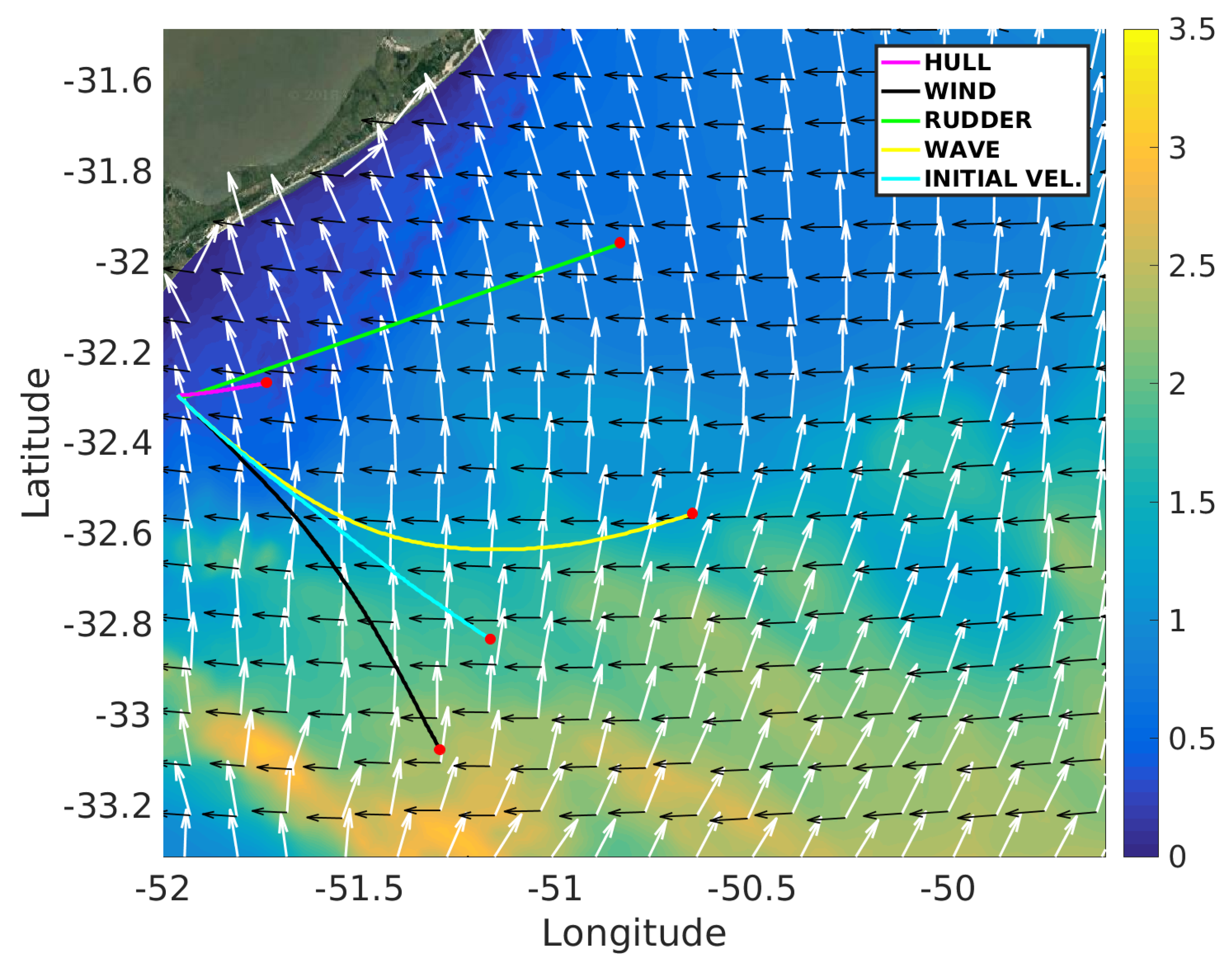
  • The ship had its trajectory deflect to starboard due to East winds, showing that wind has an influence on the ship behavior during navigation;
  • The ship had its trajectory deflect to port due to North waves; in this way the waves can influence, significantly, the ship’s route, mostly on the longer ones;
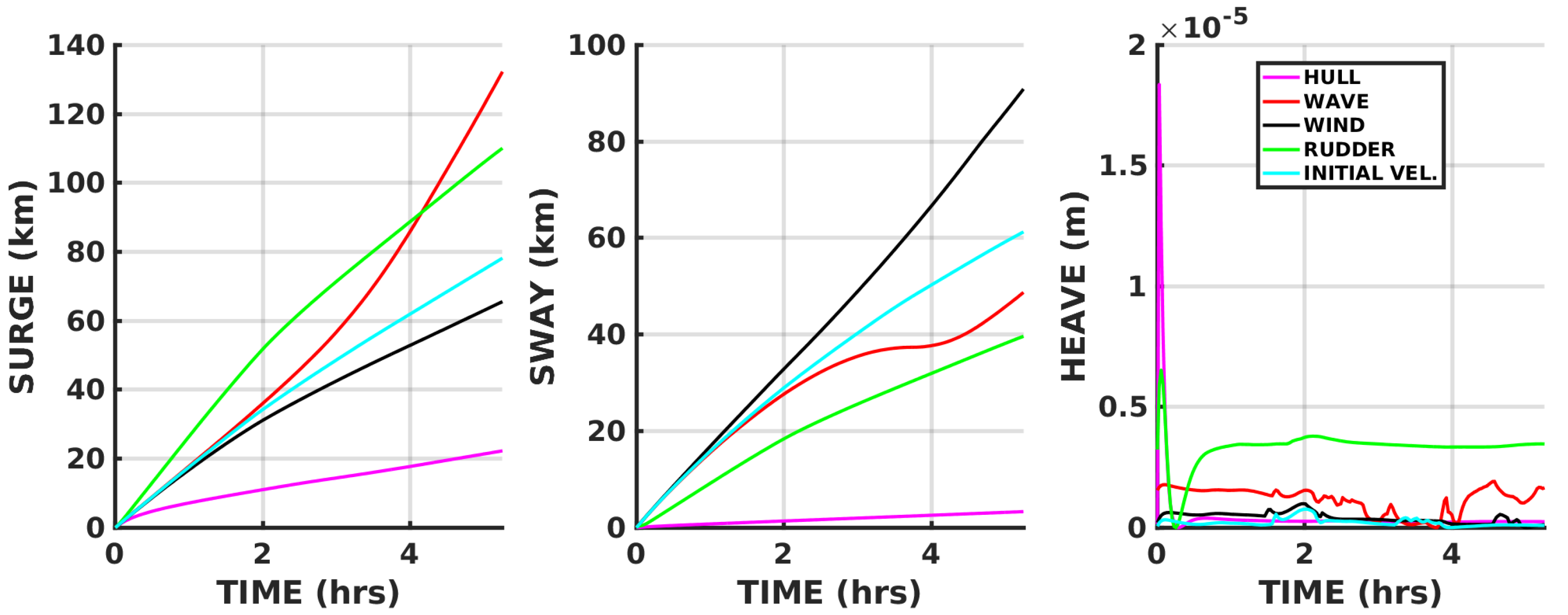
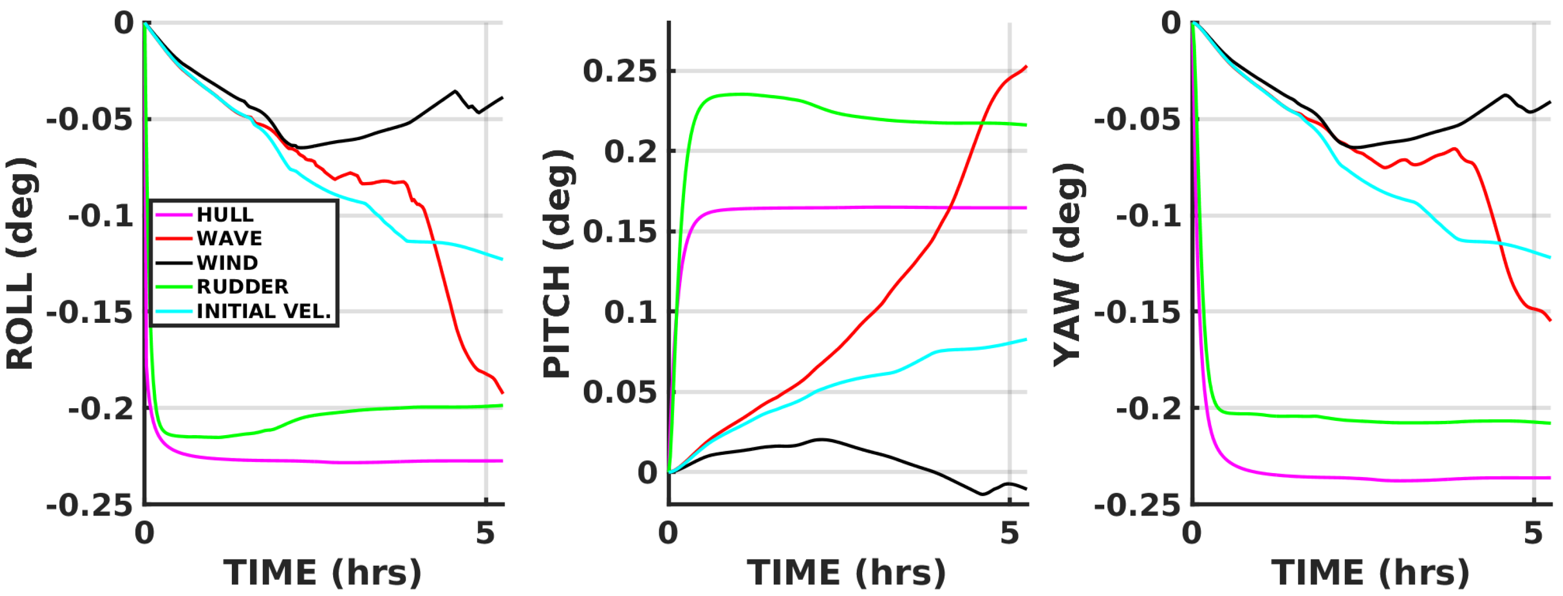
  • The wind force has no major influences in the angles of angular movements, but it can influence the ship’s trajectory mainly in longer distances;
  • The wave force can significantly deflect the vessel trajectory and it is able to affectthe angles of angular movements performed by a ship;
  • The external forces classified as MMG Model can push the vessel or make its linear movements difficult, which depends on the relative angle between the vessel and the forces;
  • The external force direction associated with high intensity of sea and wave height can deflect a ship’s trajectory or reduce its final displacement;
  • The physical characteristics of a vessel, such as mass and geometric, form can influence the performance of a ship under severe scenarios;
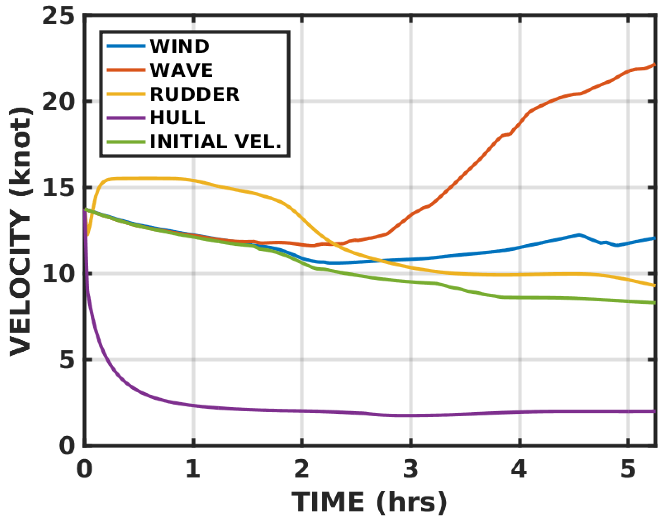
  • The velocity of a ship can significantly influence the external force magnitude, which depends on the relative velocity, including the hull and rudder forces;
From the results of this study, it can be concluded that external forces can affect significantly a ship’s trajectory, and these effects can be observed in the final trajectory, and during the trajectory also as angular movements and the ship’s instability.
As well as these results, the numerical modeling using the SHIPMOVE model can be an effective and useful tool for predicting and avoid unstable zones in the ocean, including vessel movement under various scenarios.
Moreover, the SHIPMOVE numerical model can be useful to study the influence of each external force and how researchers can improve the performance of a ship in severe scenarios.

Author Contributions

The individual contribution to this paper was performed throughout conceptualization, A.S.d.S., P.H.O., W.C.M. and E.d.P.K.; methodology, A.S.d.S., P.H.O. and J.C.; software, A.S.d.S., P.H.O. and W.C.M.; validation, A.S.d.S., P.H.O., W.C.M. and E.d.P.K.; formal analysis, P.H.O. and J.C.; investigation, P.H.O. and W.C.M.; resources, W.C.M.; data curation, A.S.d.S., P.H.O., W.C.M., J.C. and E.d.P.K.; writing—original draft preparation, A.S.d.S., P.H.O. and W.C.M.; writing—review and editing, R.C.G., J.C., A.P. and E.d.P.K.; visualization, A.S.d.S., P.H.O.; supervision, W.C.M. and E.d.P.K.; project administration, W.C.M.; funding acquisition, W.C.M.

Acknowledgments

The authors are grateful to the Conselho Nacional de Desenvolvimento Científico e Tecnológico (CNPq) under contract 146424/2017-4. Further acknowledgements go to the Brazilian Navy for providing detailed bathymetric data for the coastal area; the Brazilian National Water Agency, the PNBOIA project, NOAA, and HYCOM for supplying the validation and boundary conditions data sets, respectively; and the Open Telemac-Mascaret Consortium for freely distribution of the TELEMAC system making viable this research and finally a special thanks to the Supercomputing Center of the Federal University of Rio Grande do Sul (CESUP-UFRGS) and to the Sdumont Supercomputer from the Laboratório Nacional de Computação Científica (LNCC) (SDUMONT-2017-C01#166515) where most of the computational work was carried out. Although some data were taken from governmental databases, this paper is not necessarily representative of the views of the government.

Conflicts of Interest

The authors declare no conflict of interest.

Abbreviations

The following abbreviations are used in this manuscript:
CESUP-UFRGSSupercomputing Center of the Federal University of Rio Grande do Sul
CNPqConselho Nacional de Desenvolvimento Científico e Tecnológico
HYCOMHybrid Coordinate Ocean Model
ICIndex of Concordance
JTTCJapanese Towing Tank Conference
LANSDLaboratório de Análise Numérica e Sistemas Dinâmicos
LNCCLaboratório Nacional de Computação Científica
MAEMean Average Error
MMG ModelManeuvering Modeling Group
m o d m e a n Mean value of the model data
m o d s t d Standard deviation value of the model data
MSEMean Square Error
NANot Applied
NOAA(National Oceanic and Atmospheric Administration)
NCEPNational Centers for Environmental Prediction
NCARNational Center for Atmospheric Research
o b s m e a n Mean value of the observed data
o b s s t d Standard deviation value of the observed data
PNBOIAPrograma Nacional de Boias
RIOSResearch Initiative on Oceangoing Ships
RMSERoot Mean Square Error
R 2 Pierson error coefficient
SIScatter Index
SSMean Square Inclination
SHIPMOVESHIP MOVEMENT MODEL
TOMAWACTELEMAC-Based Operational Model Addressing Wave Action Computation

References

  1. Sclavounos, P. On the Diffraction of Free Surface Waves by a Slender Ship. Ph.D. Thesis, Massachusetts Institute of Technology, Cambridge, MA, USA, 1984. [Google Scholar]
  2. Froude, W. On the Rolling of Ships; Royal Institution of Naval Architects: London, UK, 1862; p. 95. [Google Scholar]
  3. Michell, J.H. Wave–Resistance of a Ship. Philos. Mag. 1898, 45, 106–123. [Google Scholar] [CrossRef]
  4. Maruo, H. Calculation of the Wave Resistance of Ships, the Draught of Which is as Small as the Beam. J. Zosen Kiokai 1962, 1962, 21–37. [Google Scholar] [CrossRef] [Green Version]
  5. Newman, J.N. A slender-body theory for ship oscillations in waves. J. Fluid Mech. 1964, 18, 602–618. [Google Scholar] [CrossRef]
  6. Newman, J.N.; Sclavounos, P. The Unified Theory of Ship Motions. In Proceedings of the Symposium on 13th Naval Hydrodynamics, Tokyo, Janpan, 6–10 October 1980. [Google Scholar]
  7. Moreno, C.A. Interferência Hidrodinâmica no Comportamento em ondas Entre Navios com Velocidade de Avanço. Ph.D. Thesis, Coordenação de Aperfeiçoamento de Pessoal de Nível Superior, Brasília, Brazil, 2010. [Google Scholar]
  8. Yasukawa, H.; Yoshimura, Y. Introduction of MMG standard method for ship maneuvering predictions. J. Mar. Sci. Technol. (Jpn.) 2015, 20, 37–52. [Google Scholar] [CrossRef]
  9. Ogawa, A.; Kasai, H. On the mathematical model of manoeuvring motion of ships. Int. Shipbuild. Prog. 1978, 25, 306–319. [Google Scholar] [CrossRef]
  10. Inoue, S.; Hirano, M.; Kijima, K.; Takashina, J. Practical calculation method of ship maneuvering motion. Int. Shipbuild. Prog. 1981, 28, 207–222. [Google Scholar] [CrossRef]
  11. Armudi, A.; Marques, W.; Oleinik, P. Analysis of ship behavior under influence of waves and currents. Revista de Engenharia Térmica 2017, 16, 18–26. [Google Scholar] [CrossRef]
  12. Hervouet, J.; Van Haren, L. Recent advances in numerical methods for fluid flow. In Floodplain Processes; Anderson, M.G., Walling, D.E., Bates, P.D., Eds.; Wiley: New York, NY, USA, 1996; pp. 183–214. [Google Scholar]
  13. Hervouet, J.M. Free Surface Flows: Modelling With the Finite Element Methods; John Wiley & Sons: Hoboken, NJ, USA, 2007. [Google Scholar]
  14. Millero, F.J.; Poisson, A. International one-atmosphere equation of state of seawater. Deep Sea Res. Part A Oceanogr. Res. Pap. 1981, 28, 625–629. [Google Scholar] [CrossRef]
  15. TOMAWAC. TOMAWAC Technical Report—Software for Sea State Modelling on Unstructured Grids over Oceans and Coastal Seas; Technical Report; EDF: Chateau, France, 2011. [Google Scholar]
  16. Lee, S.D.; Yu, C.H.; Hsiu, K.Y.; Hsieh, Y.F.; Tzeng, C.Y.; Kehr, Y.Z. Design and experiment of a small boat track-keeping autopilot. Ocean Eng. 2010, 37, 208–217. [Google Scholar] [CrossRef]
  17. Maimun, A.; Priyanto, A.; Rahimuddin; Sian, A.Y.; Awal, Z.I.; Celement, C.S.; Nurcholis; Waqiyuddin, M. A mathematical model on manoeuvrability of a LNG tanker in vicinity of bank in restricted water. Saf. Sci. 2013, 53, 34–44. [Google Scholar] [CrossRef]
  18. Andersen, I.M.V. Wind loads on post-panamax container ship. Ocean Eng. 2013, 58, 115–134. [Google Scholar] [CrossRef]
  19. Chen, C.; Shiotani, S.; Sasa, K. Numerical ship navigation based on weather and ocean simulation. Ocean Eng. 2013, 69, 44–53. [Google Scholar] [CrossRef] [Green Version]
  20. Zhang, W.; Zou, Z.J.; Deng, D.H. A study on prediction of ship maneuvering in regular waves. Ocean Eng. 2017, 137, 367–381. [Google Scholar] [CrossRef]
  21. Willmot, C.J. Some Comments on the Evaluation of Model Performance. Bull. Am. Meteorol. Soc. 1982, 63, 1309–1313. [Google Scholar] [CrossRef] [Green Version]
  22. Janssen, P.A.E.M.; Hansen, B.; Bidlot, J.R. Verification of the ECMWF Wave Forecasting System against Buoy and Altimeter Data. Am. Meteorol. Soc. 1997, 12, 763–784. [Google Scholar] [CrossRef]
  23. Lalbeharry, R. Evaluation of the CMC regional wave forecasting system against buoy data. Atmosphere-Ocean 2002, 40, 1–20. [Google Scholar] [CrossRef] [Green Version]
  24. Chawla, A.; Spindler, D.M.; Tolman, H.L. Validation of a thirty year wave hindcast using the Climate Forecast System Reanalysis winds. Ocean Model. 2013, 70, 189–206. [Google Scholar] [CrossRef]
  25. Teegavarapu, R.S.V. Floods in a Changing Climate: Extreme Precipitation; Cambridge University Press: Cambridge, UK, 2013; p. 268. [Google Scholar]
  26. Edwards, E.; Cradden, L.; Ingram, D.; Kalogeri, C. Verification within wave resource assessments. Part 1: Statistical analysis. Int. J. Mar. Energy 2014, 8, 50–69. [Google Scholar] [CrossRef] [Green Version]
  27. Khandekar, M. Operational Wave Models. In Guide to Wave Analysis and Forecasting, 2nd ed.; World Meteorological Association: Geneva, Switzerland, 1998; Chapter 6; pp. 67–80. [Google Scholar]
  28. Bidlot, J.R.; Holmes, D.J.; Whittmann, P.A.; Lalbeharry, R.; Chen, H.S. Intercomparison of the Performance of Operational Ocean Wave Forecasting Systems with Buoy Data. Am. Meteorol. Soc. 2002, 17. [Google Scholar] [CrossRef]
  29. Cha, R.; Wan, D. Numerical investigation of motion response of two model ships in regular waves. Procedia Eng. 2015, 116, 20–31. [Google Scholar] [CrossRef]
  30. Chuang, Z.; Steen, S. Speed loss of a vessel sailing in oblique waves. Ocean Eng. 2013, 64, 88–99. [Google Scholar] [CrossRef]
  31. Bennett, S.; Hudson, D.; Temarel, P. The influend of forward speed on ship motions in abnormal waves: Experimental measurements and numerical predictions. J. Fluids Struct. 2013, 39, 154–172. [Google Scholar] [CrossRef]
  32. Ozdemir, Y.; Barlas, B. Numerical study of ship motions and added resistance in regular incident waves of KVLCC2 model. Int. J. Nav. Archit. Ocean Eng. 2017, 9, 149–159. [Google Scholar] [CrossRef] [Green Version]
  33. Papanikolaou, A.; Alfred Mohammed, E. Stochastic uncertainty modelling for ship design loads and operational guidance. Ocean Eng. 2014, 86, 47–57. [Google Scholar] [CrossRef]
  34. Papanikolaou, A.; Fournarakis, N.; Chroni, D.; Liu, S.; Plessas, T. Simulation of the Maneuvering Behavior of Ships in Adverse Weather Conditions. In Proceedings of the 31st Symposium on Naval Hydrodynamics, Monterey, CA, USA, 16 September 2016. [Google Scholar]
1.
2.
3.
4.
5.
6.
7.
8.
Figure 1. Study area located in the South-Southeastern Brazilian Shelf. The red lines represent the oceanic liquid boundaries and the spiral represents the atmospheric surface conditions. The green dot represents the initial position of the ship. The yellow dot represents the in situ data from buoy PNBOIA-SC. Bathymetry is shown in the color bar.
Jmse 07 00072 g001
Figure 2. Time series of spectral significant wave heights (m), peak period (s) peak direction (°) from TOMAWAC (blue), and velocity intensity (m· s 1 ) from TELEMAC-3D (black), compared against the observed data from the Santa Catarina PNBOIA buoy (red).
Jmse 07 00072 g002
Figure 3. Routes performed by the ship in 5 hours of simulation.
Jmse 07 00072 g003
Figure 4. Translational movements performed by the ship.
Jmse 07 00072 g004
Figure 5. Timeline of ship’s velocity.
Jmse 07 00072 g005
Figure 6. Rotational movements performed by the ship.
Jmse 07 00072 g006
Table 1. Physical characteristics of the ship simulated in this study.
Mass (kg)Length (m)Width (m)Draught (m)
2.87 × 10 7 1733212
Table 2. Comparison between statistical metrics for wave and current data. Spectral significant wave height ( H m o ), peak period ( T p ) and current intensity (Int) analyzed among the Santa Catarina PNBOIA buoy. RMSE, MAE, Bias, m o d m e a n , o b s m e a n , m o d s t d , o b s s t d are in the same units of the parameters, SI is in percentage. NA = Not Applied.
H mo T p Int
mod mean 1.979.850.26
obs mean 1.759.100.18
mod std 0.702.530.14
obs std 0.671.400.10
RMSE0.57NA0.16
MAE0.43NA0.13
IC0.70NA0.86
MSE0.33NA0.02
Bias0.220.740.07
SI (%)3323NA
SS1.121.10NA
R 2 0.700.65NA

