A Comparison of Physical and Numerical Modeling of Homogenous Isotropic Propeller Blades


1
SINTEF Ocean, NO-7465 Trondheim, Norway
2
Norwegian University of Science and Technology (NTNU), Faculty of Engineering, Department of Marine Technology, NO-7491 Trondheim, Norway
*
Author to whom correspondence should be addressed.
†
These authors contributed equally to this work.
J. Mar. Sci. Eng. 2020, 8(1), 21; https://doi.org/10.3390/jmse8010021
Submission received: 10 December 2019
/
Revised: 24 December 2019
/
Accepted: 26 December 2019
/
Published: 3 January 2020
(This article belongs to the Special Issue Selected Papers from the Sixth International Symposium on Marine Propulsors)
Abstract
:Results of the fluid-structure co-simulations that were carried out as part of the FleksProp project are presented. The FleksProp project aims to establish better design procedures that take into account the hydroelastic behavior of marine propellers and thrusters. Part of the project is devoted to establishing good validation cases for fluid-structure interaction (FSI) simulations. More specifically, this paper describes the comparison of the numerical computations carried out on three propeller designs that were produced in both a metal and resin variant. The metal version could practically be considered rigid in model scale, while the resin variant would show measurable deformations. Both variants were then tested in open water condition at SINTEF Ocean’s towing tank. The tests were carried out at different propeller rotational speeds, advance coefficients, and pitch settings. The computations were carried out using the commercial software STAR-CCM+ and Abaqus. This paper describes briefly the experimental setup and focuses on the numerical setup and the discussion of the results. The simulations agreed well with the experiments; hence, the computational approach has been validated.
1. Introduction
The topic of hydroelastic behavior of marine propellers is nowadays often associated with the behavior of composite propellers that aim at using some sort of anisotropy to achieve some set goal. The goal may be reducing vibrations or cavitation (Young [1,2]). Already in 2001, Mouritz et al. [3] published a review article citing a quite extensive list of applications of composite materials in naval applications, including propellers, where the benefits of composite materials could offset the increased costs that are associated with their design and production. However, this paper covers isotropic propellers as a first step towards anisotropic propellers. In fact, as it will be clear further in the paper, the simulation strategy adopted here should in principle work independently whether the material is isotropic or anisotropic. The choice of starting from isotropic materials was mainly made because the production methods needed for making the model scale blades were easier than for anisotropic materials.
The elastic behavior of isotropic blades has received less attention although it may in same cases be noticeable also for full-scale metallic propellers. In the past, Atkinson and Glover [4] have shown numerically how full-scale metallic propellers could bend under the action of hydrodynamic forces to an extent that some particular propeller geometries, namely blades with large skew angles, could have some significance in terms of propeller performance. The numerical method adopted was a combination of lifting line and finite element methods (FEM) in what we would call a weak co-simulation in modern terms. Nowadays, co-simulations are increasingly carried out coupling CFD (Computational Fluid Dynamics) with FEM (Finite Element Method) code. The coupling between the two codes vary from weak to strong, according to how the two simulations communicate in terms of time increments and variables that are transferred. While this has been a research area for quite some time, modern software implementations have reached a level of maturity that makes these types of analysis attractive also at the level of industrial design engineers. The increased ease of setting up co-simulations should not however be taken as a guarantee for obtaining accurate results. In fact, the accuracy of the computations should be verified and compared with results obtained in controlled scenarios, as, for example, during open water tests in a towing tank or cavitation tunnel. Despite some recent attempts of fill in the gap [5,6], there is still a scarcity of experimental data. The validation of numerical results by means of experiments presents a series of challenges that require careful preparation and interpretation of the results. It is important to limit the scope of what can be validated by means of experiments; it is practically impossible to design experiments that allow for correctly scaling to laboratories size displacements and forces of some full-scale hydroelastic phenomenon. A thorough review of what are the limitations of mode scale experiments can be found in Young [7]. What is possible is to design experiments that allow for their correct representation in the simulation codes with the aim of validating the latter. In this paper, we present the results from experiments carried out on three propeller designs that have been produced with blades both in aluminum and in a casting resin resembling an epoxy resin, hence presenting a rigid and flexible behavior, respectively. The three propellers share the same design parameters apart from the skew distribution. The tests have been performed in a classical open-water configuration at different propeller speeds and at different pitch settings. The open-water configuration was chosen so that the hydroelastic behavior was limited to static deflection, i.e., vibrations of the blades were avoided by performing the tests in a homogenous inflow.
2. Model Tests
2.1. Propeller Geometries
Three propeller geometries were generated starting from a master geometry varying the skew distribution. The master geometry is labeled P1374 and was designed using SINTEF Ocean proprietary propeller design code AKPD by Achkinadze et al. as presented in [8,9]. Propeller P1374 has a balanced skew distribution that amounts to 23 degrees. The first variation, P1565, was obtained by removing entirely any skew distribution. In the second variation, P1566, the same total skew as propeller P1374 was kept but in an unbalanced form. The geometries of the blades are available, since the FleksProp consortium decided to allow disclosure of the geometries of the three propellers. They are reported in Appendix A, while the geometrical definition of the propellers are described in Appendix B. A visual impression of how the three propellers look like is given in Figure 1.
2.2. Production of Flexible Blades
The flexible blades were manufactured using resin casting under vacuum, which is a commonly used technique in rapid prototyping. There are several variants of the resin casting technique. In the variant that was adopted in this case, the first step is to produce a positive object that is then used to form a silicon mold where the resin is cast under vacuum and left to cure at constant temperature. Three complete controllable pitch propellers, including the hubs, were produced in aluminum according to the production standard used in SINTEF Ocean. One blade per kind was then sent to a company specializing in rapid prototyping that produced 5 copies of the blade.
According to the producer of the resin used for casting, Young’s modulus is equal to 2.2 GPa. Poisson’s ratio is not reported, but given the nature of the material, it was assumed to be equal to 0.33. The material properties reported by the producer have not been checked by mechanical testing; however, the good agreement between computations and experiments indicates that the reported values can be considered accurate.
2.3. Test Executions
The model tests have been carried in the SINTEF Ocean large towing tank between the months of February and June 2018. The setup adopted was the classical open-water configuration where the propeller is placed in front of the dynamometer. The dynamometer used in the test was a Kempf & Remmers H29 model. Figure 2 shows that only the surfaces in contact with water located on the left side of the 1-mm gap contribute to the forces measured by the dynamometer.
According to standard procedures for open-water tests, a dummy hub without blades was tested to obtain forces on the cap and hub at different velocities. The forces measured during the test with the dummy are then subtracted from the forces measured with the actual propeller to obtain what is traditionally referred to as open water curves. The traditional way of presenting the data tries to isolate the blades from the propeller. When the experimental data is to be compared with CFD results, it is more consistent to use the uncorrected (raw) force measured during the experiments and to compute the forces on the abovementioned surface on the measuring side of the gap.
The open-water tests were performed at 3 different propeller rotational speeds: 7, 9, and 11 rps in the range of advance coefficients from 0 to 1.2 in 0.2 steps for the pitch setting = 1.1 and from 0 to 1.05 in 0.15 steps for the pitch setting 0.9. Tests were also performed at = 1.2, but the results from this pitch setting have not been simulated yet.
The experimental relative uncertainity at 95% confidence for the thrust and torque coefficients has been evaluated using the methodology described in Reference [10] and found to be weakly dependent on the advance coefficient J as Figure 3 shows for P1374 at n = 7 rps. Slightly smaller values of the uncertainty were found for the other rps. The uncertainty reported here is relative only to propeller P1374, but similar values were found also for the other propellers.
3. FSI Simulations
Fluid-structure interaction (FSI), in the widest sense, is the thermomechanical interaction of one or more solid structures with an internal or surrounding fluid flow. FSI problems play prominent roles in many scientific and engineering fields, such as mechanical, aerospace, and biomedical engineering. Thanks to the recent advances of commercial software, numerical simulations have become a feasible and efficient way to investigate the fundamental physics involved in the complex interaction between fluids and solids. Nevertheless, there is still the need for validation when these tools are used in new applications.
When using a numerical procedure, an FSI problem is usually described in terms of a fluid domain and a structural domain, communicating through an in-between fluid-structure interface. This multi-physics problem with adjacent domains can be simulated in a monolithic or in a partitioned way [11]: the former simultaneously solves the governing equations for fluid and structure within a unified algorithm, and it requires a code developed for this particular combination of physical problems. In the partitioned approach, on the other hand, the fluid and the structure are treated as two computational fields which can be solved separately with their respective mesh discretizations and numerical algorithms, and the boundary conditions at the interface are used explicitly to transfer information between the fluid and structure solutions. The partitioned approach enables the use of existing well-established fluid and structural solvers. This represents a significant motivation for adopting this approach in addition to the fact that, for many problems, the staggered approach works well, is very efficient, and preserves software modularity. Difficulties may arise, however, in terms of robustness and accuracy for specific problems like flutters or parachute problems [12,13].
In the present case, we consider the problem of viscous incompressible fluid flow interacting with an elastic body (the propeller blade) immersed in the flow and being deformed by the fluid action. A staggered approach is used, coupling two different solvers that use different methods and codes: a CFD/FVM (Computational Fluid Dynamics/Finite Volume Method) solver for fluids and FEA/FEM (Finite Element Analysis/Method) for structure mechanics.
In “two way” FSI, the results of the CFD solver, in terms of hydrodynamic forces on the interface, are mapped from the fluid model to the structural model and are provided to the structural equation solver; the results obtained by the structural solver are mapped back to the first model in terms of displacements of the interfacial surface, involving the modification/morphing of the mesh of the fluid model. The procedure is repeated until convergence. How often this mapping needs to be performed depends on the degrees of coupling, and it is related to the response times of the structure compared to the fluid: in case of strong coupling, the mapping may be needed in the internal time-step iterations inside each time step, following an implicit method.
In the present case, the fluid and structure are “weakly” coupled because the response of the structure to a disturbance in the fluid is slow compared to the fluid. As seen from the experiments, a “static” solution is expected, which means that one can search for a steady-state condition, corresponding to the shape the structure takes in the stationary fluid when it reaches the hydroelastic equilibrium, corresponding to the steady-state flow around the deformed blade. All these considerations have important consequences on the flexible-blade simulations:
- explicit algorithm can be used, which means that the fluid and the structure solvers are not necessarily in the processor memory at the same time and that the mapping between the two codes may happen at each time-step (and not at each internal iteration)
- the analysis does not need to be time accurate, as an equilibrium state with a static solution is desired
- material damping can be increased
- first-order integration in time may be used
Numerical Setup
In the present work, STAR-CCM+ v12.04 by Siemens PLM Software [14] is used as CFD code and Abaqus 2016 by Dassault Systèmes is used as FEM code. An open-water simulation was used as a starting point, with the following characteristics: the computational domain is corresponding to one-blade passage only, the MRF (Multi-Reference Frame) approach is used. Using the MRF approach means that the propeller rotation is not simulated with the actual rotation of the mesh but that it is modeled using a reference system rotating with the blades. The equations of motion are solved in this reference system, once the boundary conditions have been correctly set up on the propeller surfaces with the proper value of velocity.
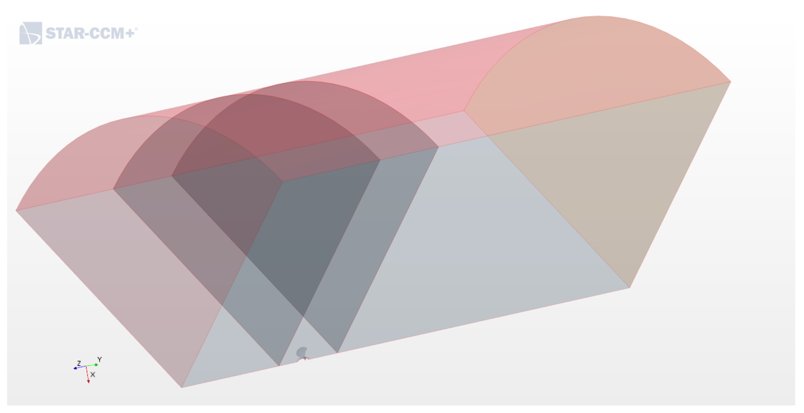
The computational domain and boundary conditions are illustrated in Figure 4 and Figure 5. It is a sector of a cylinder, of which the axis corresponds to the propeller axis of rotation and radius equal to 10 propeller diameters. The propeller is located in the region highlighted in red in Figure 5, where a polyhedral mesh is generated and then extruded further upstream and downstream toward the inlet and outlet boundary respectively.
The geometry of the numerical propeller model is kept as close as possible to the one used in the experiments, including the gap of 1 mm between the hub and the cone; the housing is modeled with infinite length, extended up to the outlet.
A longitudinal section of the volume mesh is depicted in Figure 6. The mesh for all the considered cases consists of about cells, including 10 layers of prismatic layers at the wall. The thickness of the first prismatic layer is set to approximately have of the order of 1 on the blades. The Gamma–ReTheta transition model is used for turbulence, which performed better than the Shear Stress Turbulent (SST)-K- and the Reynolds Stress Turbulent (RST) models; the reason is because, at the model scale, there are likely areas of the blades subjected to laminar flow with transition to turbulent flow.
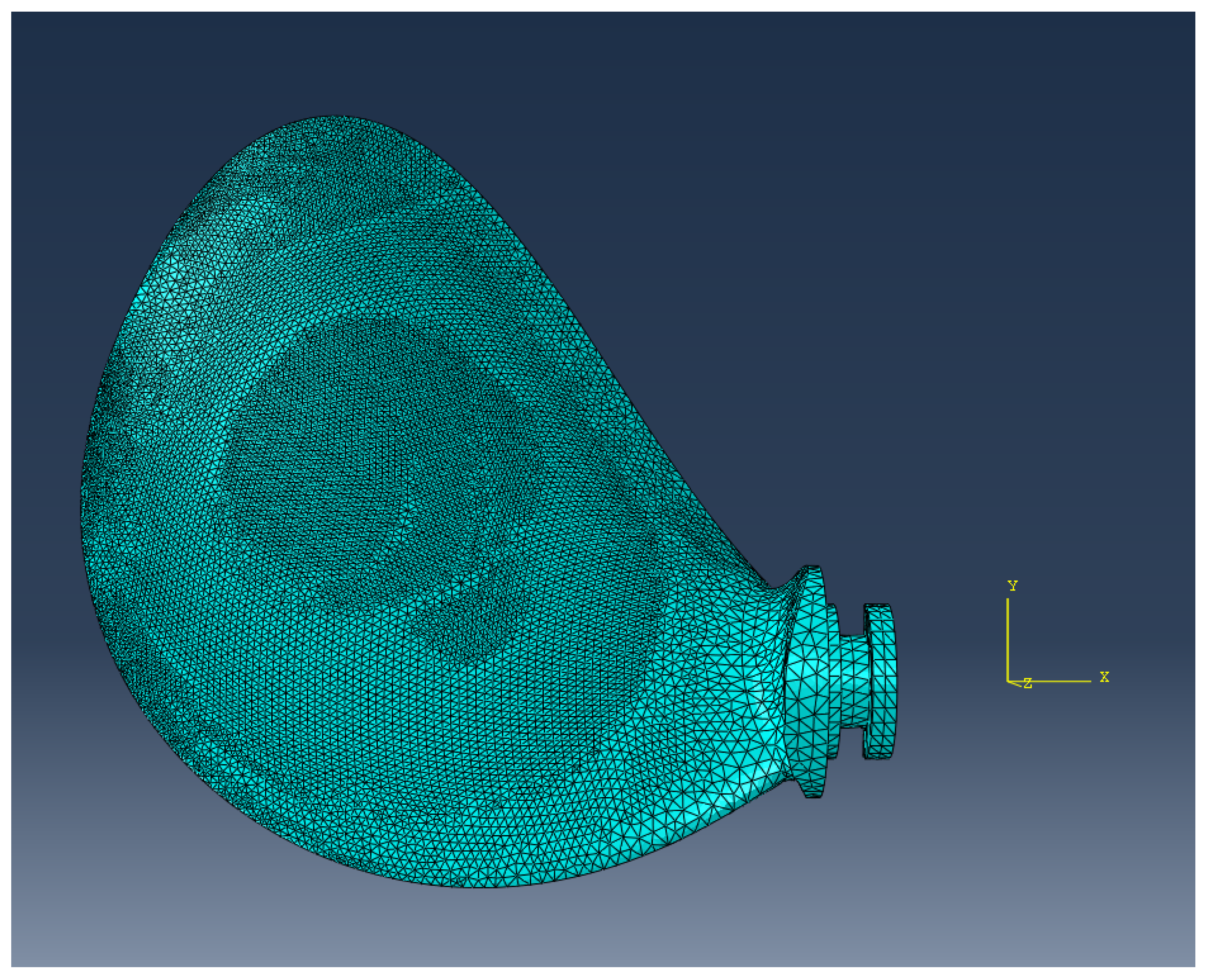
The structural mesh consisted of tetrahedral elements and was generated by the Abaqus embedded mesher. To determine the number of cells that was necessary for a correct structural simulation, a mesh refinement study was performed where the mesh was refined until the displacements at the blade tip were no longer changing with the mesh size. Mesh refinements were applied at the leading and trailing edges of the blade. While the mesh target size was set to 0.5 mm, the mesh refinement at the edges dominated the mesh size as it can be seen in Figure 7, where the structural mesh of propeller P1565 is shown as an example.
For the structural part of the computations, it is important to model the root of the blade and the fastening system. The blade root is built in the same resin as the rest of the blade and has several contact surfaces that constrain it to the propeller hub. The different contact surfaces determine different boundary conditions. In Figure 8, the different boundary conditions are identified with different colors; the red surfaces are an encastre-type boundary condition, while the green surface identifies a surface that allows only rotation along the direction perpendicular to the surface and translations in the plane identified by the surface.
The three propellers designs, P1374, P1566, and P1565, are analyzed. Initially the open-water calculations are carried out for the rigid case, with reference to the model tests with the aluminium propellers. The resulting flow field is then used as initial flow state for the CFD-FEM co-simulations, activating the Abaqus and the morpher solvers.
The mapping is managed by StarCCM+, where the co-simulation setup is accomplished by identifying the coupled model parts and the exported/imported fields (pressure/displacements) and by specifying the external code execution details (commands, input files, etc.).
4. Results
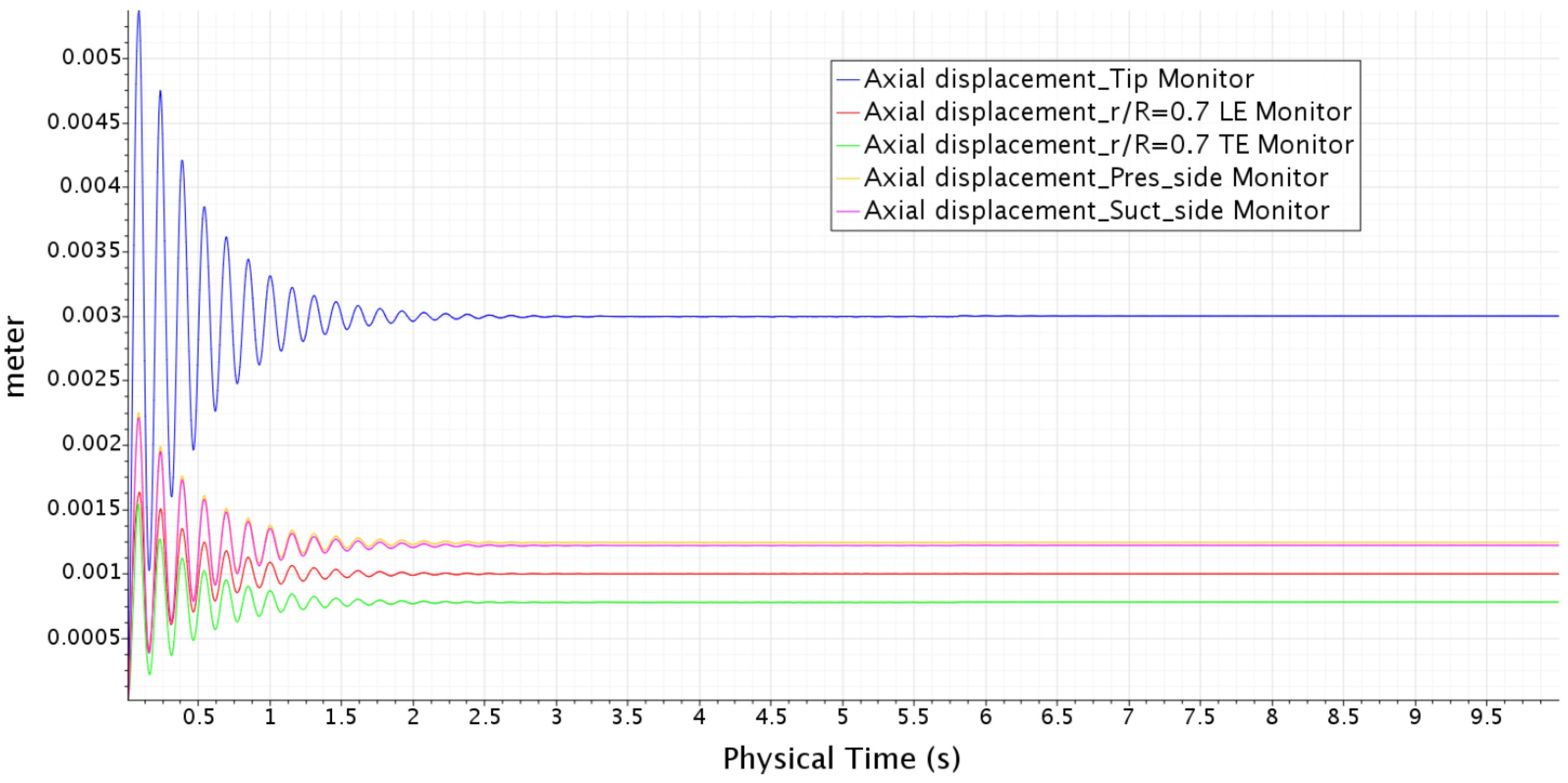
A converged solution of the co-simulation is reached well before the simulation time, initially fixed to , with time step of , as shown in Figure 9, where the axial displacements at different locations of the blade are monitored during the simulation for the propeller P1374, P/, and . The results obtained for the three propellers at and are reported in Figure 10 and Figure 11, respectively: , , and obtained by the co-simulation are plotted as a function of the advance ratio J both for the aluminum propeller and for the (flexible) resin propeller and compared to the experimental values. The agreement is very satisfactory, also in terms of the relative increase of the coefficients in the flexible case with respect to the rigid one. Except for the bollard condition and for the case, where the blades can experience flow with “negative” angle of attack and subsequent separation and unsteadiness, the difference between the numerical results and the experimental data is less than in terms of thrust coefficients, as shown for example in Figure 12, where the differences for , , and are shown for the propeller P1374, . Note that, with reference to Figure 3, the deviation seen between CFD and experiments is, in most cases, within the uncertainty bands of the experiments. The only case where the deviations seem to be large is for the propeller efficiency at and ; however, it should be noted that the coefficient is slightly negative, leading to a negative efficiency, which is strictly speaking not consistent with the definition of propeller efficiency, and hence, the propeller efficiency for that specific condition should be disregarded; further, the thrust and torque coefficients are correctly captured by the simulations.
Blade Displacements
It is rather straightforward to extract the blade cylindrical section displacements from the numerical computations and to compare the effect of the different skew distributions of the three blades. One way that seems quite natural is to decompose the displacements of the sections in terms of bending and twisting. In this approximation, the bend is defined as the average displacement of the blade sections in the YZ plane, where Z is the propeller advance direction, X is the radial direction, and Y is the direction perpendicular to both X and Z. Twist is defined as the rotation of the blade section in the same YZ plane. Some results for this twist definition are shown in Figure 13 and Figure 14. Close to the tip, the twist component is correctly identified, while erroneous results appear closer to the blade root. Still, this presentation will be used here since it offers a compact way of presenting the data. Note also that the reservations on the bend-twist presentation of the data apply only to twist.
It was expected that the elastic behavior of the low aspect ratio propeller blades could only partially be represented by pure bend and twist of the blade sections. It is important to keep in mind this finding when trying to implement design codes that are based on lower order theories, as for example lifting line theory coupled with beam theory. It may be beneficial to consider also the warping in addition to the bending and twisting of the blade sections, as shown in Figure 14.
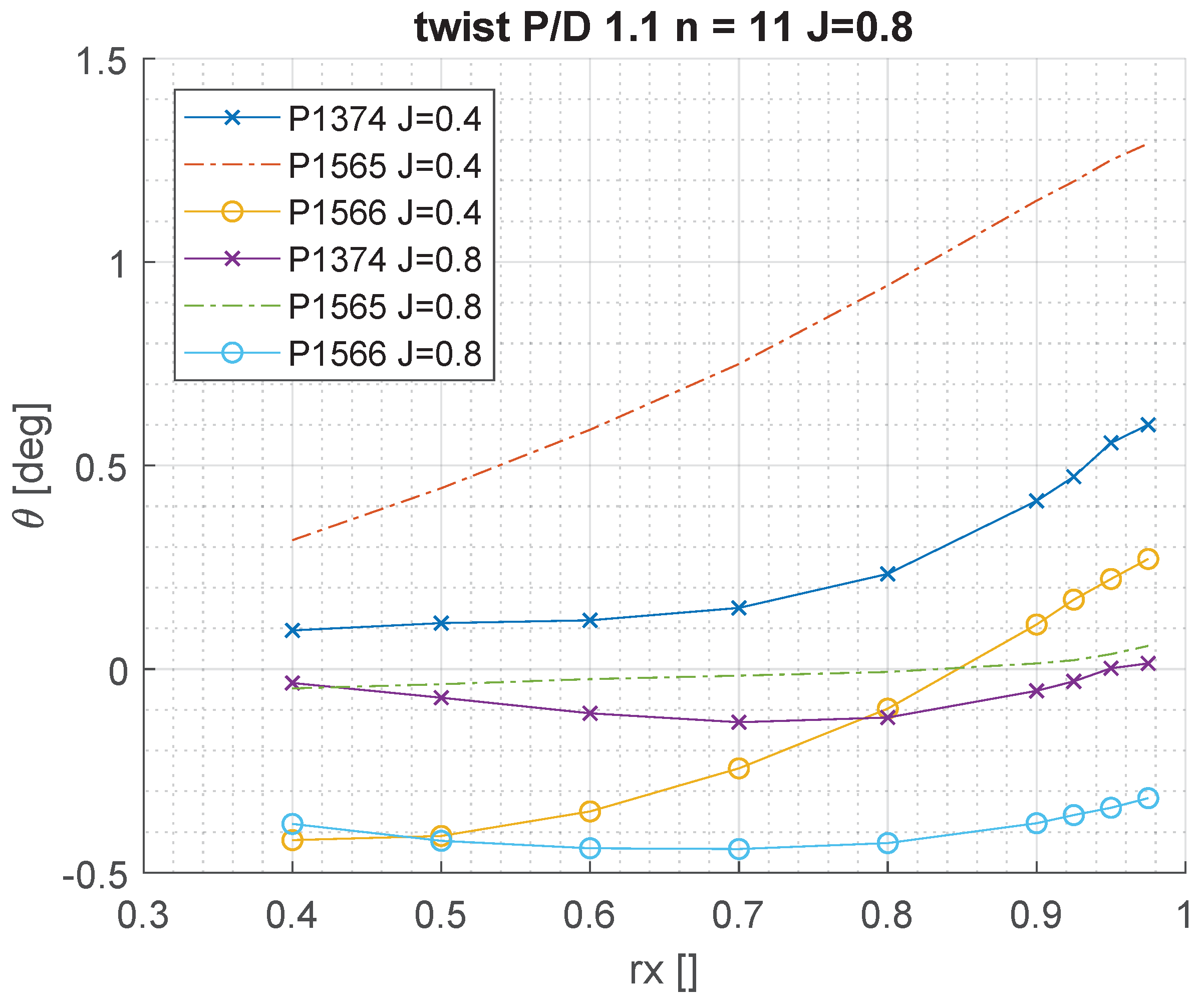
Even with the reservation that has just been described, it is possible to use the bend-twist approximation to explain the effect of the propeller skew on propeller blades that are otherwise identical. In Figure 15 and Figure 16, the bend and twist of the sections from the radial location 0.4 to 0.975 are plotted.
Although it may appear to an extent fictitious, since the skew distribution is often used to control cavitation and little room is left for other uses of it, in a hypothetical case where cavitation is not a concern, it may be in principle possible to think using the skew distribution to achieve an hydroelastic response of some sort. The mechanism by which the bend and twist are coupled in isotropic materials is the so-called geometrical bend twist coupling. In the geometrical bend twist coupling, the skew distribution influences the relative position of the pressure center and the elastic center leading to different elastic behaviors even for the same, for the sake of simplicity, uniform pressure distribution. In reality, the skew distribution influences also the pressure distribution on the blade, but in a first approximation, we assume the geometrical bend-twist coupling as the main driving factor for the different behavior of the three geometries. In Figure 15 and Figure 16, the bend and twist distribution along the blade radius for the three propellers at two operating conditions are shown. The operating conditions are chosen to be close to the design point and an off-design condition where the propeller is heavy-loaded. Not surprisingly, the different skew distributions of the three geometries have limited effects on the propeller bending, while the effect is clearly seen on the twist of blade sections. The blade section twist is defined as positive if, as a result of the deformation, the blade section ends up having a larger pitch than in the unloaded condition. At a design point, the balanced skew (P1374) and the zero skew (P1565) propellers are subjected to almost no twist while the unbalanced skew propeller (P1566) has a slight negative twist. In the off-design condition, the skew distribution affects to a larger extent the elastic behavior of the propellers; in this condition, all blades show a twist distribution that is increasing from the root towards the tip of the blade. The zero skew blade shows an almost linear, comparatively large twist of the blade sections. The two blade designs with skew show a somewhat similar behavior with the section towards the tip, bending considerably more than those at the root. Even though, as it has already been pointed out, the bend-twist decomposition of the blade deformation may not be accurate especially for the sections close to the blade root, a few conclusion can be drawn. The first conclusion is that it is indeed possible to use the skew distribution to obtain an hydroelastic bend-twist coupling for isotropic materials. The second conclusion, at least for the geometries that have been tested, it is that the bend-twist coupling that is obtained is hardly useful for achieving the goals that are typically expected from self-adaptive blades; in fact, all the skew distributions tend to show a tendency to increasing the twist angle and, hence, the pitch, with increasing loading, a result that is the opposite of what is generally desirable. These result are far from being surprising; however, it may be useful in some special applications to consider geometric bend-twist coupling as well when designing isotropic blades that are expected to work in off-design conditions.
5. Discussion
In this paper, the validation of fluid-structure interaction computations for flexible propeller blades carried out using the co-simulation approach has been described. The validation data come from a series of ad hoc tests performed with the specific aim of serving as a reference for numerical computations. For the experiments, three propellers were manufactured both in a metallic and plastic material in order to have rigid and flexible models. The propeller geometries and the experimental data are public domain and can be obtained upon request. The simulated values of thrust and torque coefficients lie mostly within the bands of experimental uncertainty, showing how CFD-FEM co-simulations can be used to accurately represent the behavior of homogeneous isotropic blades tested in open water. Furthermore, the thrust coefficients seem to compare better than the torque coefficients. It is often reported that, in model-scale CFD simulation, the torque coefficient suffers from deviation that are larger than those observed on the thrust coefficient, a phenomenon that is often attributed to the laminar-to-turbulent transition of the flow on the model-scale blades. Since the Reynolds numbers of full-scale propellers are higher, it is to be expected that CFD can better predict the full-scale torque coefficient, since the flow is mainly turbulent, a fact that makes the approach described here even more valuable. Finally, in the paper, it is shown that warping of the blade sections towards the root of the blade may be a better representation of the actual deformation of the blade than twist.
Author Contributions
Conceptualization, L.S. (Luca Savio) and L.S. (Lucia Sileo); methodology, L.S. (Lucia Sileo); software, L.S. (Lucia Sileo) and S.K.Å.; validation, L.S. (Luca Savio); resources, L.S. (Luca Savio); writing—review and editing, L.S. (Lucia Sileo), L.S. (Luca Savio), and S.K.Å.; project administration, L.S. (Luca Savio); funding acquisition, L.S. (Luca Savio). All authors have read and agreed to the published version of the manuscript.
Funding
This research was funded by Research Council of Norway and Kongsberg Maritime grant number 267495/O80.
Acknowledgments
The present work has been fully supported by the FleksProp project. The FleksProp project is a cooperation between SINTEF Ocean, the Norwegian University of Science and Technology NTNU, and Kongsberg Maritime with the economic support of the Research Council of Norway (RCN) and Kongsberg Maritime. The economic support of the Research Council of Norway and Kongsberg Maritime is greatly appreciated.
Conflicts of Interest
The authors declare no conflict of interest.
Abbreviations
The following abbreviations are used in this manuscript:
| FSI | Fluid-Structure Interaction |
| CFD | Computational Fluid Dynamics |
| FVM | Finite Volume Method |
| FEA | Finite Element Analysis |
| FEM | Finite Element Method |
| MRF | Multi-Reference Frame |
| SST | Shear Stress Turbulent model |
| RST | Reynolds Stress Turbulent model |
| rps | revolutions per second |
Appendix A. Propeller Geometry
Appendix A.1. P1374
Main propeller elements
- Propeller diameter................................ : 250.000 (mm)
- Hub diameter........................................ : 60.000 (mm)
- Number of blades..................................: 4
- Expanded area ratio..............................: 0.602
- Expanded “total” skew angle..............: 23.067 (deg.)

Table A1.
Main geometrical parameters of propeller P1374.
| - | mm | mm | mm | mm | mm | mm | mm | mm | mm | deg |
|---|---|---|---|---|---|---|---|---|---|---|
| r/R | r | Lfor | Laft | b | cs | xr | eo | fo | P | Fi |
| 0.24 | 30 | 16.67 | −16.67 | 33.35 | 0 | 0 | 9.51 | 0.28 | 269.5 | 55.03 |
| 0.25 | 31.25 | 18.12 | −17.22 | 35.34 | 0.45 | 0 | 9.38 | 0.85 | 269.74 | 53.95 |
| 0.3 | 37.5 | 25.21 | −19.78 | 44.99 | 2.71 | 0 | 8.68 | 1.69 | 270.84 | 48.98 |
| 0.35 | 43.75 | 31.96 | −22.13 | 54.09 | 4.91 | 0 | 8 | 2.19 | 271.81 | 44.68 |
| 0.4 | 50 | 38.26 | −24.34 | 62.6 | 6.96 | 0 | 7.35 | 2.56 | 272.66 | 40.96 |
| 0.5 | 62.5 | 48.98 | −28.62 | 77.6 | 10.18 | 0 | 6.12 | 3.08 | 273.96 | 34.9 |
| 0.6 | 75 | 55.93 | −33.46 | 89.39 | 11.24 | 0 | 5 | 3.35 | 274.74 | 30.24 |
| 0.7 | 87.5 | 57.33 | −39.65 | 96.98 | 8.84 | 0 | 3.98 | 3.36 | 275 | 26.57 |
| 0.8 | 100 | 50.68 | −47.81 | 98.49 | 1.44 | 0 | 3.05 | 3 | 272.05 | 23.41 |
| 0.9 | 112.5 | 31.88 | −57.23 | 89.1 | −12.68 | 0 | 2.23 | 2.08 | 259.41 | 20.15 |
| 0.95 | 118.75 | 14.71 | −60.34 | 75.05 | −22.81 | 0 | 1.85 | 1.35 | 248.38 | 18.41 |
| 0.975 | 121.88 | 1.87 | −59.42 | 61.29 | −28.77 | 0 | 1.68 | 0.9 | 241.52 | 17.51 |
| 0.99 | 123.75 | −9.69 | −55.61 | 45.92 | −32.65 | 0 | 1.56 | 0.54 | 236.97 | 16.95 |
| 0.995 | 124.38 | −15.66 | −52.31 | 36.65 | −33.99 | 0 | 1.54 | 0.38 | 235.39 | 16.76 |
| 1 | 125 | −25.99 | −44.74 | 18.75 | −35.36 | 0 | 1.5 | 0 | 233.75 | 16.57 |
Appendix A.2. P1565
Main propeller elements
- Propeller diameter................................ : 250.000 (mm)
- Hub diameter........................................ : 60.000 (mm)
- Number of blades..................................: 4
- Expanded area ratio..............................: 0.602
- Expanded “total” skew angle..............: 0.0 (deg.)
Table A2.
Main geometrical parameters of propeller P1565.
| - | mm | mm | mm | mm | mm | mm | mm | mm | mm | deg |
|---|---|---|---|---|---|---|---|---|---|---|
| r/R | r | Lfor | Laft | b | cs P1566 | xr | eo | fo | P | Fi |
| 0.24 | 30 | 16.67 | −16.67 | 33.35 | 0 | 0 | 9.51 | 0.28 | 269.5 | 55.03 |
| 0.25 | 31.25 | 17.67 | −17.67 | 35.34 | 0 | 0 | 9.38 | 0.85 | 269.74 | 53.95 |
| 0.3 | 37.5 | 22.49 | −22.49 | 44.99 | 0 | 0 | 8.68 | 1.69 | 270.84 | 48.98 |
| 0.35 | 43.75 | 27.04 | −27.04 | 54.09 | 0 | 0 | 8 | 2.19 | 271.81 | 44.68 |
| 0.4 | 50 | 31.3 | −31.3 | 62.6 | 0 | 0 | 7.35 | 2.56 | 272.66 | 40.96 |
| 0.5 | 62.5 | 38.8 | −38.8 | 77.6 | 0 | 0 | 6.12 | 3.08 | 273.96 | 34.9 |
| 0.6 | 75 | 44.69 | −44.69 | 89.39 | 0 | 0 | 5 | 3.35 | 274.74 | 30.24 |
| 0.7 | 87.5 | 48.49 | −48.49 | 96.98 | 0 | 0 | 3.98 | 3.36 | 275 | 26.57 |
| 0.8 | 100 | 49.24 | −49.24 | 98.49 | 0 | 0 | 3.05 | 3 | 272.05 | 23.41 |
| 0.9 | 112.5 | 44.55 | −44.55 | 89.1 | 0 | 0 | 2.23 | 2.08 | 259.41 | 20.15 |
| 0.95 | 118.75 | 37.53 | −37.53 | 75.05 | 0 | 0 | 1.85 | 1.35 | 248.38 | 18.41 |
| 0.975 | 121.88 | 30.64 | −30.64 | 61.29 | 0 | 0 | 1.68 | 0.9 | 241.52 | 17.51 |
| 0.99 | 123.75 | 22.96 | −22.96 | 45.92 | 0 | 0 | 1.56 | 0.54 | 236.97 | 16.95 |
| 0.995 | 124.38 | 18.32 | −18.32 | 36.65 | 0 | 0 | 1.54 | 0.38 | 235.39 | 16.76 |
| 1 | 125 | 9.38 | −9.38 | 18.75 | 0 | 0 | 1.5 | 0 | 233.75 | 16.57 |
Appendix A.3. P1566
Main propeller elements
- Propeller diameter................................ : 250.000 (mm)
- Hub diameter........................................ : 60.000 (mm)
- Number of blades..................................: 4
- Expanded area ratio..............................: 0.602
- Expanded “total” skew angle..............: 23.000 (deg.)
Table A3.
Main geometrical parameters of propeller P1566.
| - | mm | mm | mm | mm | mm | mm | mm | mm | mm | deg |
|---|---|---|---|---|---|---|---|---|---|---|
| r/R | r | Lfor | Laft | b | cs P1565 | xr | eo | fo | P | Fi |
| 0.24 | 30 | 16.67 | −16.67 | 33.35 | 0 | 0 | 9.51 | 0.28 | 269.5 | 55.03 |
| 0.25 | 31.25 | 17.39 | −17.95 | 35.34 | −0.28 | 0 | 9.38 | 0.85 | 269.74 | 53.95 |
| 0.3 | 37.5 | 20.68 | −24.3 | 44.99 | −1.81 | 0 | 8.68 | 1.69 | 270.84 | 48.98 |
| 0.35 | 43.75 | 23.47 | −30.62 | 54.09 | −3.58 | 0 | 8 | 2.19 | 271.81 | 44.68 |
| 0.4 | 50 | 25.71 | −36.9 | 62.6 | −5.59 | 0 | 7.35 | 2.56 | 272.66 | 40.96 |
| 0.5 | 62.5 | 28.34 | −49.27 | 77.6 | −10.46 | 0 | 6.12 | 3.08 | 273.96 | 34.9 |
| 0.6 | 75 | 28.19 | −61.2 | 89.39 | −16.51 | 0 | 5 | 3.35 | 274.74 | 30.24 |
| 0.7 | 87.5 | 24.72 | −72.26 | 96.98 | −23.77 | 0 | 3.98 | 3.36 | 275 | 26.57 |
| 0.8 | 100 | 17.01 | −81.48 | 98.49 | −32.23 | 0 | 3.05 | 3 | 272.05 | 23.41 |
| 0.9 | 112.5 | 2.77 | −86.33 | 89.1 | −41.78 | 0 | 2.23 | 2.08 | 259.41 | 20.15 |
| 0.95 | 118.75 | −9.41 | −84.46 | 75.05 | −46.94 | 0 | 1.85 | 1.35 | 248.38 | 18.41 |
| 0.975 | 121.88 | −18.97 | −80.26 | 61.29 | −49.61 | 0 | 1.68 | 0.9 | 241.52 | 17.51 |
| 0.99 | 123.75 | −28.29 | −74.21 | 45.92 | −51.25 | 0 | 1.56 | 0.54 | 236.97 | 16.95 |
| 0.995 | 124.38 | −33.47 | −70.12 | 36.65 | −51.8 | 0 | 1.54 | 0.38 | 235.39 | 16.76 |
| 1 | 125 | −42.98 | −61.73 | 18.75 | −52.35 | 0 | 1.5 | 0 | 233.75 | 16.57 |
Appendix A.4. Blade Section Profiles for P1374/P1565/P1566
Blade section profiles
x/b—chordwise coordinate, [0;1]; Yu, Yl—ordinates of the upper/lower sides of the profile,
Yc—ordinates of the profile mean line, given in mm
Table A4.
Geometry of the blade sections—P1374/P1565/P1566.
| r/R | x/b | 0 | 0.005 | 0.0075 | 0.0125 | 0.025 | 0.05 | 0.1 | 0.2 | 0.3 | 0.4 | 0.5 | 0.6 | 0.7 | 0.8 | 0.9 | 0.95 | 1 |
|---|---|---|---|---|---|---|---|---|---|---|---|---|---|---|---|---|---|---|
| Yu | 0 | 0.65 | 0.81 | 1.05 | 1.47 | 2.06 | 2.86 | 3.89 | 4.53 | 4.91 | 5.03 | 4.9 | 4.42 | 3.52 | 2.1 | 1.24 | 0.3 | |
| 0.24 | Yl | 0 | −0.62 | −0.77 | −1 | −1.39 | −1.91 | −2.62 | −3.5 | −4.06 | −4.38 | −4.48 | −4.36 | −3.93 | −3.14 | −1.9 | −1.14 | −0.3 |
| Yc | 0 | 0.01 | 0.02 | 0.03 | 0.04 | 0.07 | 0.12 | 0.19 | 0.24 | 0.26 | 0.28 | 0.27 | 0.25 | 0.19 | 0.1 | 0.05 | 0 | |
| Yu | 0 | 0.66 | 0.83 | 1.09 | 1.55 | 2.19 | 3.08 | 4.24 | 4.97 | 5.39 | 5.54 | 5.39 | 4.87 | 3.88 | 2.29 | 1.34 | 0.3 | |
| 0.25 | Yl | 0 | −0.59 | −0.73 | −0.93 | −1.28 | −1.73 | −2.32 | −3.05 | −3.5 | −3.75 | −3.83 | −3.72 | −3.36 | −2.68 | −1.66 | −1.02 | −0.3 |
| Yc | 0 | 0.04 | 0.05 | 0.08 | 0.14 | 0.23 | 0.38 | 0.6 | 0.74 | 0.82 | 0.85 | 0.83 | 0.76 | 0.6 | 0.31 | 0.16 | 0 | |
| Yu | 0 | 0.65 | 0.82 | 1.09 | 1.57 | 2.27 | 3.26 | 4.56 | 5.38 | 5.86 | 6.03 | 5.88 | 5.32 | 4.23 | 2.46 | 1.42 | 0.3 | |
| 0.3 | Yl | 0 | −0.51 | −0.62 | −0.78 | −1.04 | −1.35 | −1.74 | −2.19 | −2.45 | −2.6 | −2.64 | −2.56 | −2.3 | −1.85 | −1.21 | −0.8 | −0.3 |
| Yc | 0 | 0.07 | 0.1 | 0.15 | 0.27 | 0.46 | 0.76 | 1.18 | 1.46 | 1.63 | 1.69 | 1.66 | 1.51 | 1.19 | 0.62 | 0.31 | 0 | |
| Yu | 0 | 0.63 | 0.79 | 1.06 | 1.55 | 2.27 | 3.28 | 4.64 | 5.5 | 6.01 | 6.19 | 6.03 | 5.46 | 4.35 | 2.51 | 1.44 | 0.3 | |
| 0.35 | Yl | 0 | −0.44 | −0.53 | −0.66 | −0.86 | −1.08 | −1.32 | −1.58 | −1.72 | −1.8 | −1.81 | −1.75 | −1.57 | −1.27 | −0.9 | −0.64 | −0.3 |
| Yc | 0 | 0.09 | 0.13 | 0.2 | 0.35 | 0.59 | 0.98 | 1.53 | 1.89 | 2.1 | 2.19 | 2.14 | 1.94 | 1.54 | 0.81 | 0.4 | 0 | |
| Yu | 0 | 0.6 | 0.76 | 1.02 | 1.51 | 2.23 | 3.26 | 4.65 | 5.53 | 6.05 | 6.23 | 6.08 | 5.5 | 4.38 | 2.52 | 1.44 | 0.3 | |
| 0.4 | Yl | 0 | −0.38 | −0.46 | −0.56 | −0.7 | −0.84 | −0.97 | −1.07 | −1.11 | −1.13 | −1.12 | −1.07 | −0.95 | −0.79 | −0.64 | −0.5 | −0.3 |
| Yc | 0 | 0.11 | 0.15 | 0.23 | 0.41 | 0.69 | 1.15 | 1.79 | 2.21 | 2.46 | 2.56 | 2.5 | 2.27 | 1.8 | 0.94 | 0.47 | 0 | |
| Yu | 0 | 0.54 | 0.69 | 0.94 | 1.41 | 2.11 | 3.14 | 4.53 | 5.42 | 5.95 | 6.14 | 5.99 | 5.42 | 4.32 | 2.48 | 1.41 | 0.3 | |
| 0.5 | Yl | 0 | −0.28 | −0.33 | −0.38 | −0.43 | −0.45 | −0.39 | −0.23 | −0.11 | −0.03 | 0.01 | 0.03 | 0.05 | 0 | −0.21 | −0.28 | −0.3 |
| Yc | 0 | 0.13 | 0.18 | 0.28 | 0.49 | 0.83 | 1.38 | 2.15 | 2.66 | 2.96 | 3.08 | 3.01 | 2.74 | 2.16 | 1.13 | 0.57 | 0 | |
| Yu | 0 | 0.47 | 0.61 | 0.84 | 1.28 | 1.95 | 2.94 | 4.28 | 5.15 | 5.66 | 5.85 | 5.71 | 5.17 | 4.13 | 2.36 | 1.35 | 0.3 | |
| 0.6 | Yl | 0 | −0.19 | −0.22 | −0.24 | −0.22 | −0.14 | 0.06 | 0.4 | 0.63 | 0.78 | 0.85 | 0.85 | 0.78 | 0.58 | 0.11 | −0.11 | −0.3 |
| Yc | 0 | 0.14 | 0.2 | 0.3 | 0.53 | 0.91 | 1.5 | 2.34 | 2.89 | 3.22 | 3.35 | 3.28 | 2.98 | 2.35 | 1.23 | 0.62 | 0 | |
| Yu | 0 | 0.41 | 0.53 | 0.73 | 1.13 | 1.74 | 2.65 | 3.89 | 4.69 | 5.17 | 5.34 | 5.22 | 4.73 | 3.78 | 2.16 | 1.25 | 0.3 | |
| 0.7 | Yl | 0 | −0.12 | −0.13 | −0.12 | −0.07 | 0.08 | 0.36 | 0.8 | 1.1 | 1.29 | 1.37 | 1.35 | 1.24 | 0.94 | 0.31 | −0.01 | −0.3 |
| Yc | 0 | 0.14 | 0.2 | 0.3 | 0.53 | 0.91 | 1.5 | 2.35 | 2.9 | 3.23 | 3.36 | 3.28 | 2.98 | 2.36 | 1.24 | 0.62 | 0 | |
| Yu | 0 | 0.33 | 0.43 | 0.6 | 0.93 | 1.45 | 2.22 | 3.28 | 3.96 | 4.37 | 4.52 | 4.42 | 4 | 3.21 | 1.85 | 1.09 | 0.3 | |
| 0.8 | Yl | 0 | −0.08 | −0.08 | −0.06 | 0.02 | 0.17 | 0.46 | 0.91 | 1.21 | 1.39 | 1.47 | 1.45 | 1.33 | 1 | 0.36 | 0.02 | −0.3 |
| Yc | 0 | 0.13 | 0.18 | 0.27 | 0.48 | 0.81 | 1.34 | 2.1 | 2.59 | 2.88 | 3 | 2.93 | 2.66 | 2.11 | 1.1 | 0.55 | 0 | |
| Yu | 0 | 0.24 | 0.31 | 0.43 | 0.66 | 1.03 | 1.57 | 2.32 | 2.8 | 3.08 | 3.19 | 3.11 | 2.82 | 2.28 | 1.35 | 0.83 | 0.3 | |
| 0.9 | Yl | 0 | −0.06 | −0.06 | −0.05 | −0.01 | 0.1 | 0.29 | 0.59 | 0.79 | 0.91 | 0.96 | 0.95 | 0.87 | 0.64 | 0.18 | −0.07 | −0.3 |
| Yc | 0 | 0.09 | 0.12 | 0.19 | 0.33 | 0.56 | 0.93 | 1.45 | 1.79 | 2 | 2.08 | 2.03 | 1.85 | 1.46 | 0.77 | 0.38 | 0 | |
| Yu | 0 | 0.18 | 0.23 | 0.32 | 0.49 | 0.75 | 1.14 | 1.66 | 2 | 2.2 | 2.28 | 2.22 | 2.01 | 1.64 | 1.02 | 0.66 | 0.3 | |
| 0.95 | Yl | 0 | −0.07 | −0.07 | −0.08 | −0.06 | −0.02 | 0.07 | 0.23 | 0.33 | 0.4 | 0.43 | 0.42 | 0.39 | 0.26 | −0.02 | −0.16 | −0.3 |
| Yc | 0 | 0.06 | 0.08 | 0.12 | 0.21 | 0.37 | 0.61 | 0.95 | 1.17 | 1.3 | 1.35 | 1.32 | 1.2 | 0.95 | 0.5 | 0.25 | 0 | |
| Yu | 0 | 0.15 | 0.19 | 0.26 | 0.39 | 0.59 | 0.89 | 1.28 | 1.53 | 1.68 | 1.74 | 1.69 | 1.53 | 1.26 | 0.82 | 0.56 | 0.3 | |
| 0.975 | Yl | 0 | −0.07 | −0.09 | −0.1 | −0.11 | −0.11 | −0.08 | −0.02 | 0.02 | 0.05 | 0.06 | 0.06 | 0.06 | 0 | −0.15 | −0.23 | −0.3 |
| Yc | 0 | 0.04 | 0.05 | 0.08 | 0.14 | 0.24 | 0.4 | 0.63 | 0.78 | 0.86 | 0.9 | 0.88 | 0.8 | 0.63 | 0.33 | 0.17 | 0 | |
| Yu | 0 | 0.13 | 0.16 | 0.22 | 0.32 | 0.47 | 0.69 | 0.98 | 1.17 | 1.28 | 1.32 | 1.29 | 1.17 | 0.97 | 0.66 | 0.48 | 0.3 | |
| 0.99 | Yl | 0 | −0.08 | −0.1 | −0.12 | −0.15 | −0.18 | −0.21 | −0.23 | −0.24 | −0.24 | −0.24 | −0.23 | −0.21 | −0.21 | −0.26 | −0.28 | −0.3 |
| Yc | 0 | 0.02 | 0.03 | 0.05 | 0.09 | 0.15 | 0.24 | 0.38 | 0.47 | 0.52 | 0.54 | 0.53 | 0.48 | 0.38 | 0.2 | 0.1 | 0 | |
| Yu | 0 | 0.12 | 0.15 | 0.2 | 0.29 | 0.42 | 0.61 | 0.86 | 1.02 | 1.11 | 1.15 | 1.12 | 1.01 | 0.85 | 0.6 | 0.45 | 0.3 | |
| 0.995 | Yl | 0 | −0.09 | −0.11 | −0.13 | −0.17 | −0.22 | −0.27 | −0.33 | −0.37 | −0.39 | −0.39 | −0.38 | −0.34 | −0.32 | −0.32 | −0.31 | −0.3 |
| Yc | 0 | 0.02 | 0.02 | 0.03 | 0.06 | 0.1 | 0.17 | 0.26 | 0.33 | 0.36 | 0.38 | 0.37 | 0.33 | 0.26 | 0.14 | 0.07 | 0 | |
| Yu | 0 | 0.1 | 0.12 | 0.16 | 0.23 | 0.31 | 0.43 | 0.58 | 0.68 | 0.73 | 0.75 | 0.73 | 0.66 | 0.56 | 0.42 | 0.34 | 0.25 | |
| 1 | Yl | 0 | −0.1 | −0.12 | −0.16 | −0.23 | −0.31 | −0.43 | −0.58 | −0.68 | −0.73 | −0.75 | −0.73 | −0.66 | −0.56 | −0.42 | −0.34 | −0.25 |
| Yc | 0 | 0 | 0 | 0 | 0 | 0 | 0 | 0 | 0 | 0 | 0 | 0 | 0 | 0 | 0 | 0 | 0 |
Appendix B. AKPD/AKPA Geometrical Definitions and Sign Conventions
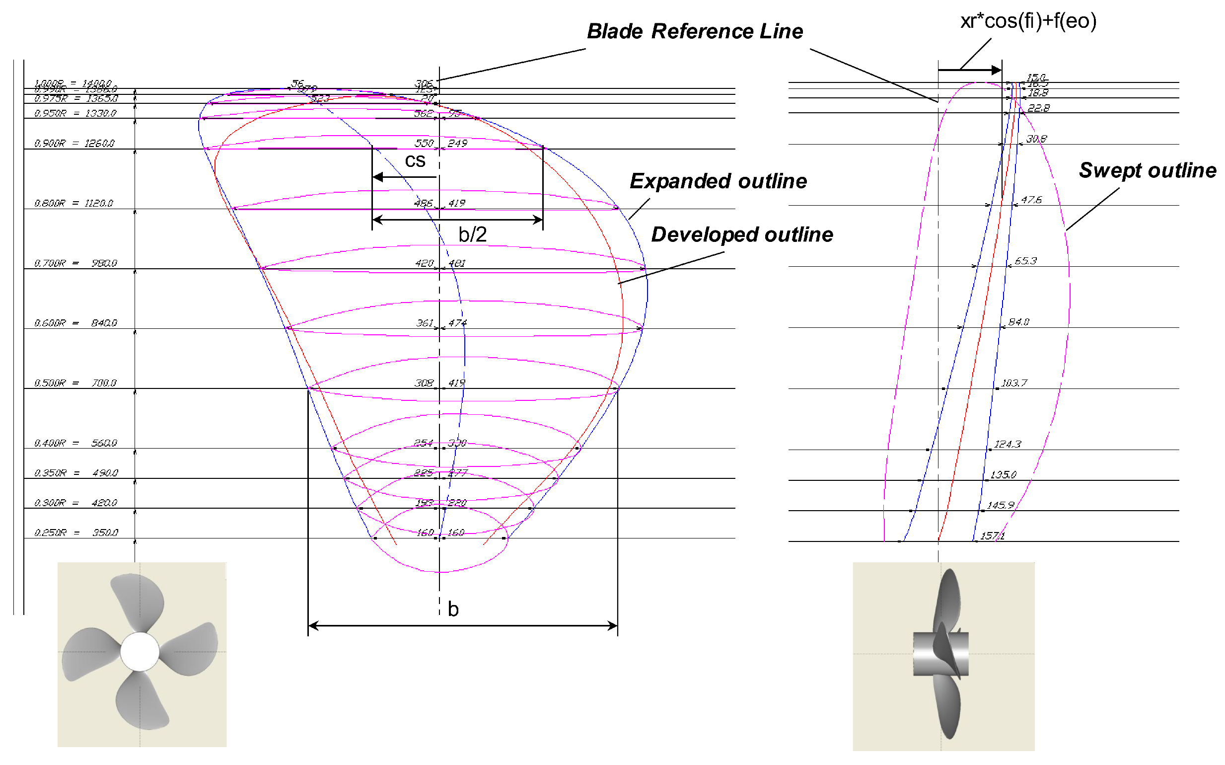
Figure A1.
AKPD-AKPA geometrical definitions.

Figure A2.
AKPD-AKPA geometrical definitions.
References
- Young, Y.L. Fluid-structure interaction analysis of flexible composite marine propellers. J. Fluids Struct. 2008, 24, 799–818. [Google Scholar] [CrossRef]
- Young, Y.L.; Garg, N.; Brandner, P.A.; Pearce, B.W.; Butler, D.; Clarke, D.; Phillips, A.W. Load-dependent bend-twist coupling effects on the steady-state hydroelastic response of composite hydrofoils. Compos. Struct. 2018, 189, 398–418. [Google Scholar] [CrossRef]
- Mouritz, P.; Gellert, E.; Burchill, P.; Challis, K. Review of advanced composite structures for naval ships and submarines. Compos. Struct. 2001, 53, 21–42, ISSN 0263-8223. [Google Scholar] [CrossRef]
- Atkinson, P.; Glover, E.J. Propeller hydroelastic effects. In Proceedings of the Propellers 88 Symposium, Virginia Beach, VA, USA, 20–21 September 1988. [Google Scholar]
- Savio, L. Measurements of the deflection of a flexible propeller blade by means of stereo imaging. In Proceedings of the SMP2015—The Fourth International Symposium on Marine Propulsors, Austin, TX, USA, 31 May–4 June 2015. [Google Scholar]
- Maljaars, P.; Bronswijk, L.; Windt, J.; Grasso, N.; Kaminski, M. Experimental Validation of Fluid-Structure Interaction Computations of Flexible Composite Propellers in Open Water Conditions Using BEM-FEM and RANS-FEM Methods. J. Mar. Sci. Eng. 2018, 6, 51. [Google Scholar] [CrossRef] [Green Version]
- Young, Y.L. Dynamic hydroelastic scaling of self-adaptive composite marine rotors. Compos. Struct. 2010, 92, 97–106. [Google Scholar] [CrossRef]
- Achkinadze, A.S.; Krasilnikov, V.I. A Numerical Lifting-Surface Technique for Account of Radial Velocity Component in Screw Propeller Design Problem. In Proceedings of the 7th International Conference on Numerical Ship Hydrodynamic NSH7, Nantes, France, 19–22 July 1999. [Google Scholar]
- Achkinadze, A.S.; Krasilnikov, V.I.; Stepanov, I.E. A Hydrodynamic Design Procedure for Multi-Stage Blade-Row Propulsors Using Generalized Linear Model of the Vortex Wake. In Proceedings of the Propellers/Shafting’2000 SNAME Symposium, Virginia Beach, VA, USA, 20–21 September 2000. [Google Scholar]
- JCGM. JCGM 100:2008. GUM 1995 with Minor Corrections-Valuation of Measurement Data—Guide to the Expression of Uncertainty in Measurement; JCGM: Paris, France, 2008. [Google Scholar]
- Hou, G.; Wang, J.; Layton, A. Numerical Methods for Fluid-Structure Interaction—A Review. Commun. Comput. Phys. 2012, 12, 337–377. [Google Scholar] [CrossRef]
- Bazilevs, Y.; Calo, V.M.; Hughes, T.J.; Zhang, Y. Isogeometric fluid-structure interaction: Theory, algorithms, and computations. Comput. Mech. 2008, 43, 3–37. [Google Scholar] [CrossRef]
- Degroote, J.; Haelterman, R.; Annerel, S.; Bruggeman, P.; Vierendeels, J. Performance of partitioned procedures in fluid–structure interaction. Comput. Struct. 2010, 88, 446–457. [Google Scholar] [CrossRef] [Green Version]
- Siemens PLM Software. STAR-CCM+ v12.04 User Guide; Siemens PLM Software: Plano, TX, USA, 2017. [Google Scholar]
Figure 1.
Outline of the three geometries showing the different skew distributions.
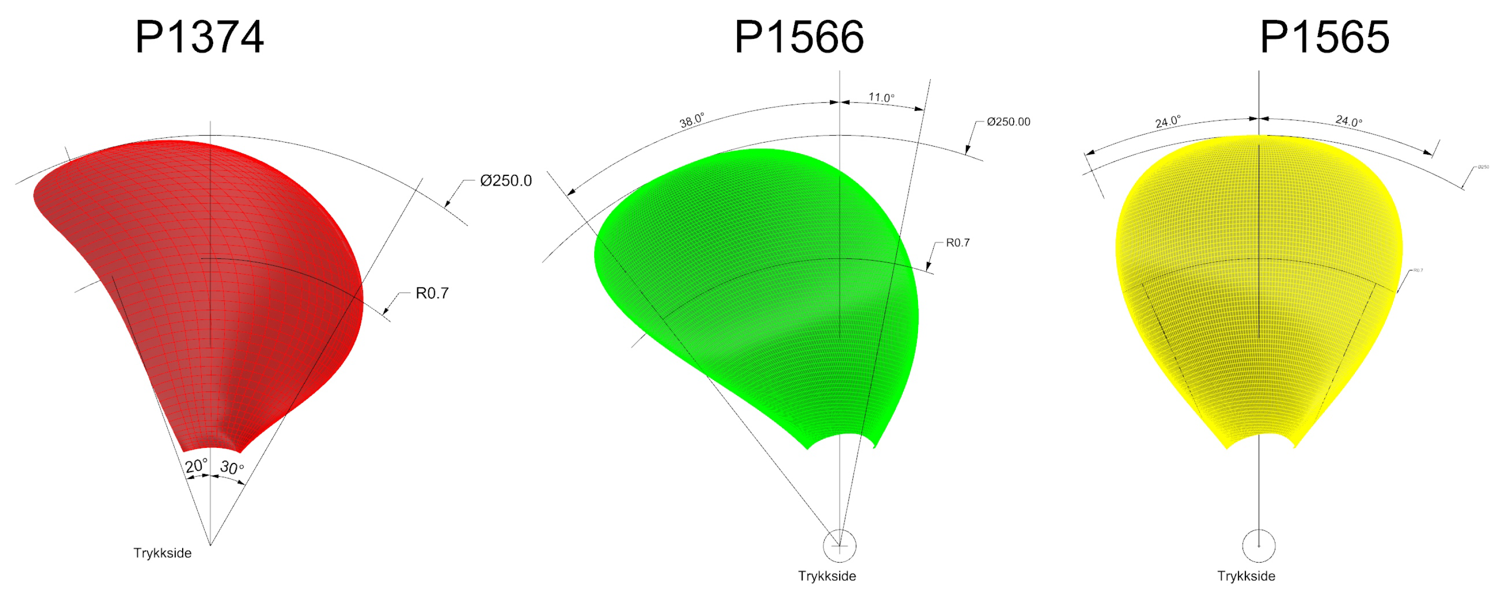
Figure 2.
Experimental setup showing which surfaces contribute to the forces measured during the experiments.
Figure 2.
Experimental setup showing which surfaces contribute to the forces measured during the experiments.
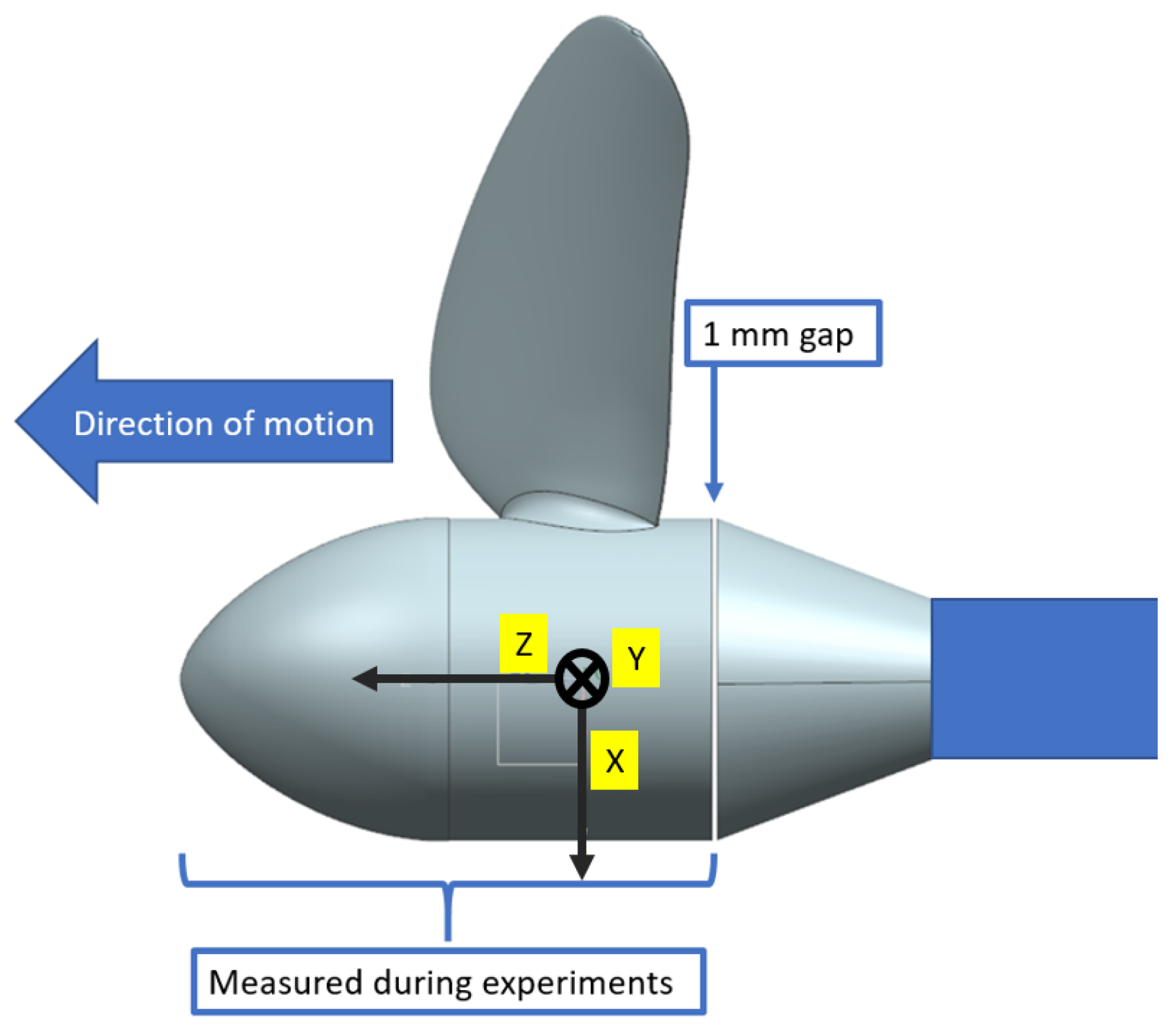
Figure 3.
Example of relative uncertainity for propeller P1374 at 1.1 and n = 7.
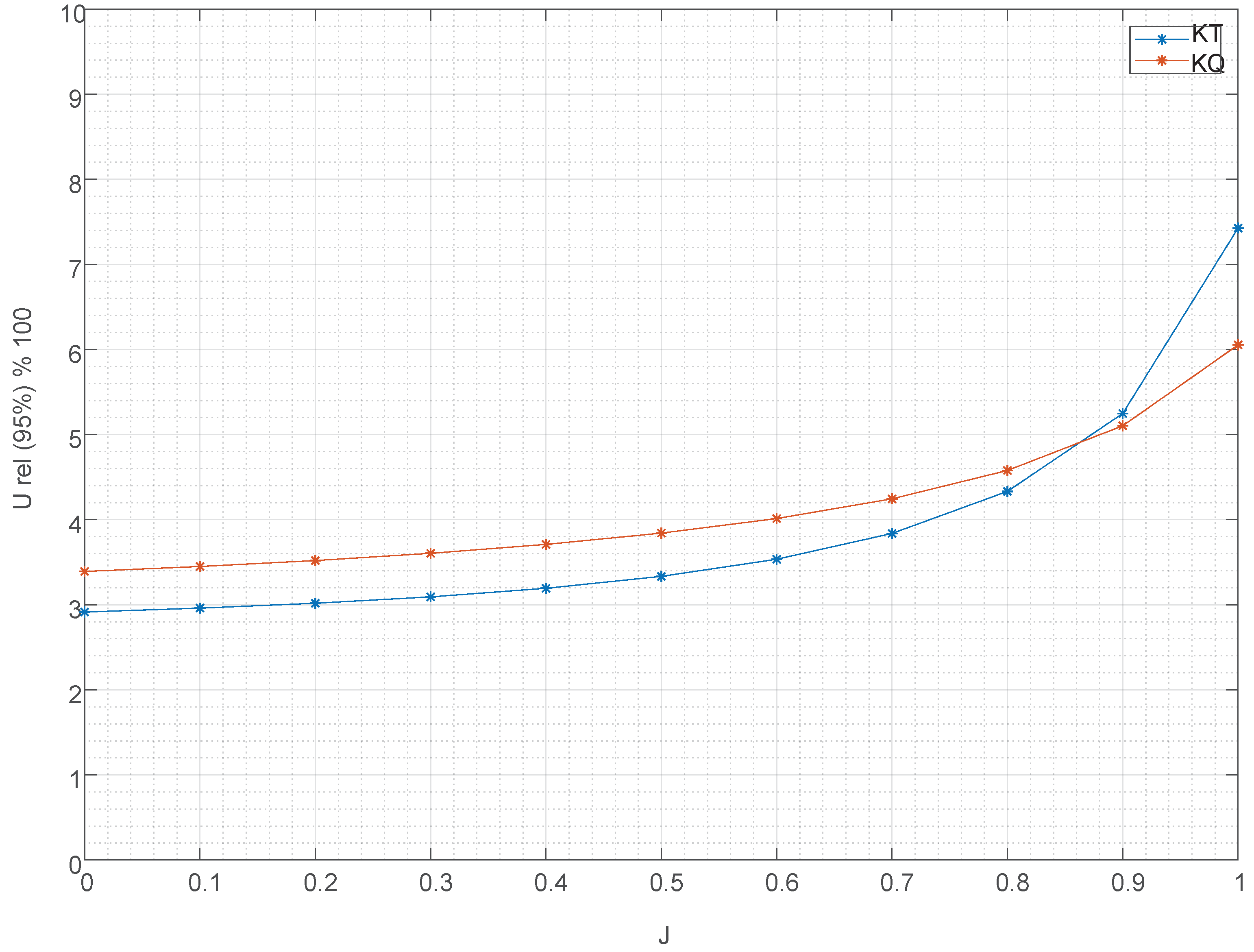
Figure 4.
Computational domain used in the simulation: The picture shows the size of the computational domain compared to the blade size. Note the fact that only one of the four blades was simulated.
Figure 4.
Computational domain used in the simulation: The picture shows the size of the computational domain compared to the blade size. Note the fact that only one of the four blades was simulated.

Figure 5.
Domain size and boundary conditions: The figure depicts the domain size in terms of propeller diameters and the function of the different blocks used in the meshing procedure.
Figure 5.
Domain size and boundary conditions: The figure depicts the domain size in terms of propeller diameters and the function of the different blocks used in the meshing procedure.

Figure 6.
Longitudinal section of the volume mesh of the fluid dynamic solver.

Figure 7.
As an example of the mesh used by the strucural solver, the mesh relative to propeller P1565 is presented.
Figure 7.
As an example of the mesh used by the strucural solver, the mesh relative to propeller P1565 is presented.

Figure 8.
Boundary condition at the blade root: The color codes can be found in the text.

Figure 9.
Propeller P1374, , and rps: axial displacements at different locations of the blade monitored during the simulation.
Figure 9.
Propeller P1374, , and rps: axial displacements at different locations of the blade monitored during the simulation.

Figure 10.
Results for : The results are presented in a matrix form where the different geometries are arranged in rows and the rps is in columns. The continuous lines are relative to the experimental results, while the dots are relative to the simulations. Further, the dashed lines refer to the aluminum models and the solid lines refer to the resin models; the hollow dots are relative to the computation with the rigid propeller, whereas the the solid dots are relative to the flexible propeller.
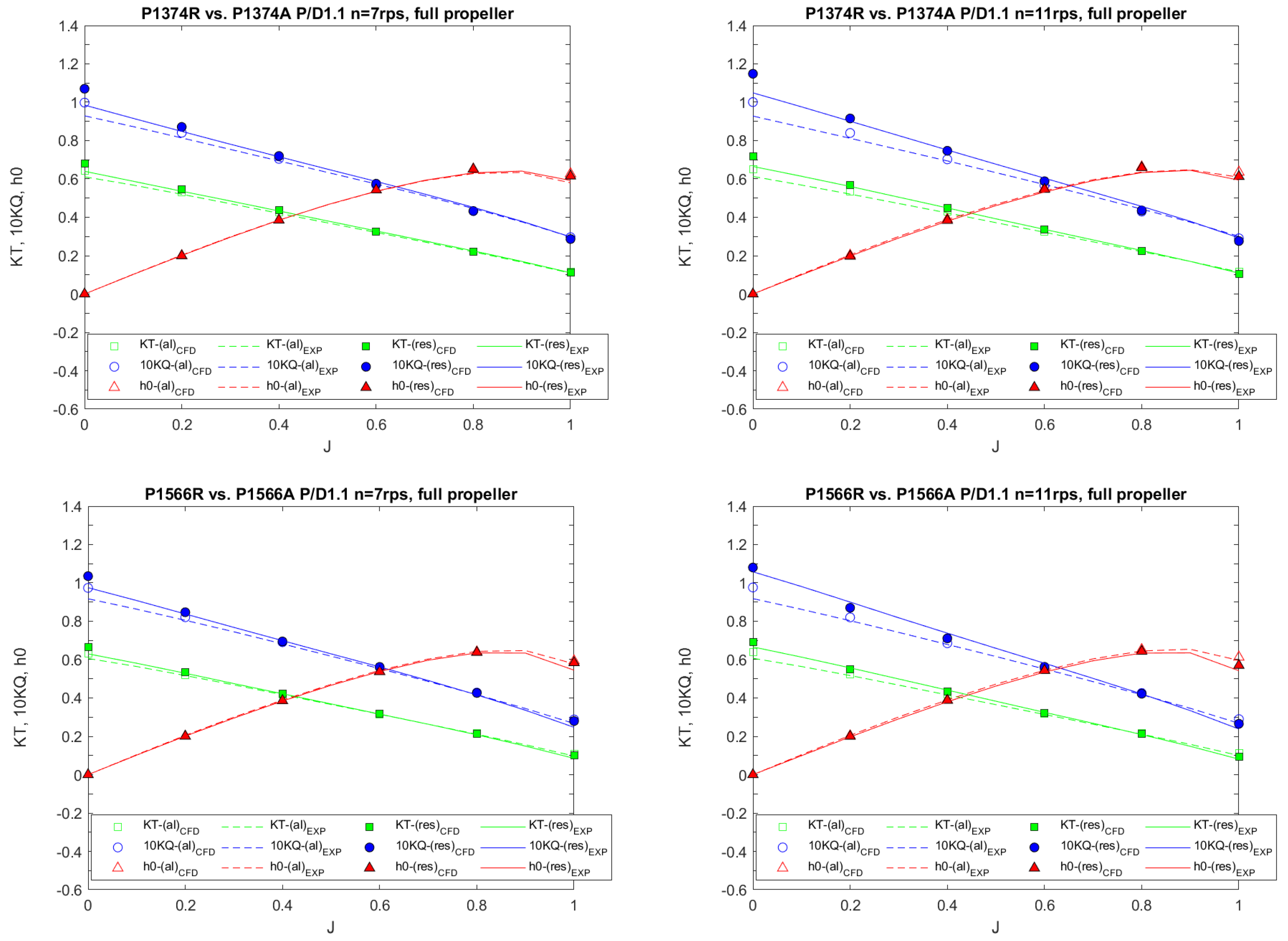
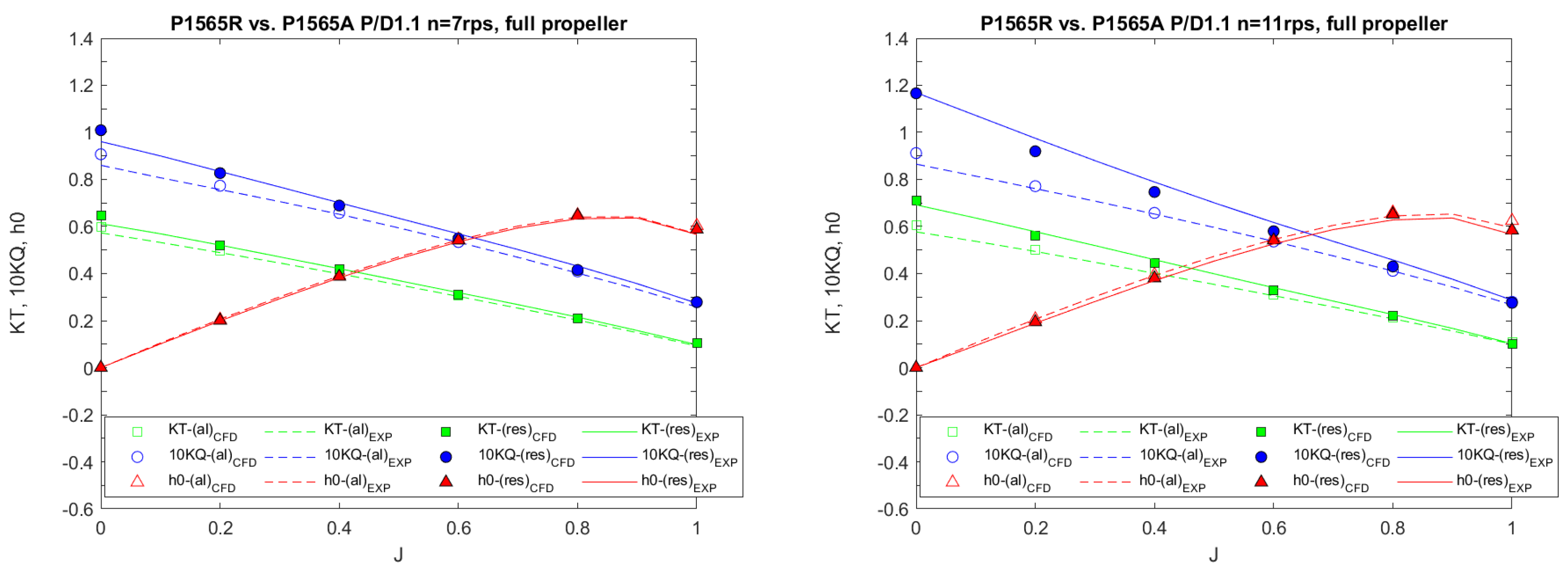
Figure 11.
Results of : The results are presented in a matrix form where the different geometries are arranged in rows and the rps is in columns. The continuous lines are relative to the experimental results, while the dots are relative to the simulations. Further, the dashed lines refer to the aluminum models and the solid lines refer to the resin models; the hollow dots are relative to the computation with the rigid propeller, whereas the the solid dots are relative to the flexible propeller.
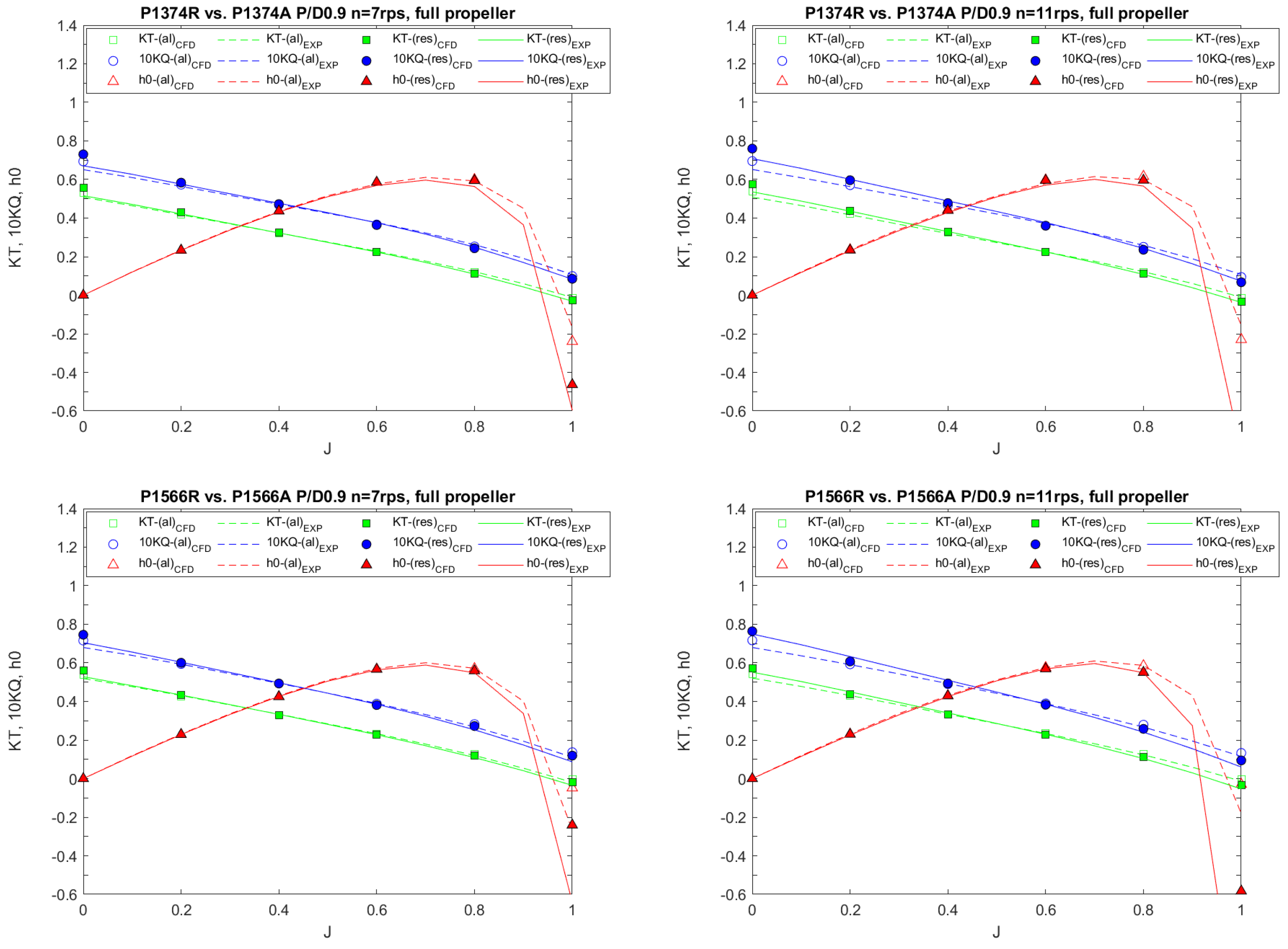

Figure 12.
Propeller P1374, , , and : relative differences between numerical and experimental data in terms of thrust and torque coefficients and propeller efficiency.
Figure 12.
Propeller P1374, , , and : relative differences between numerical and experimental data in terms of thrust and torque coefficients and propeller efficiency.
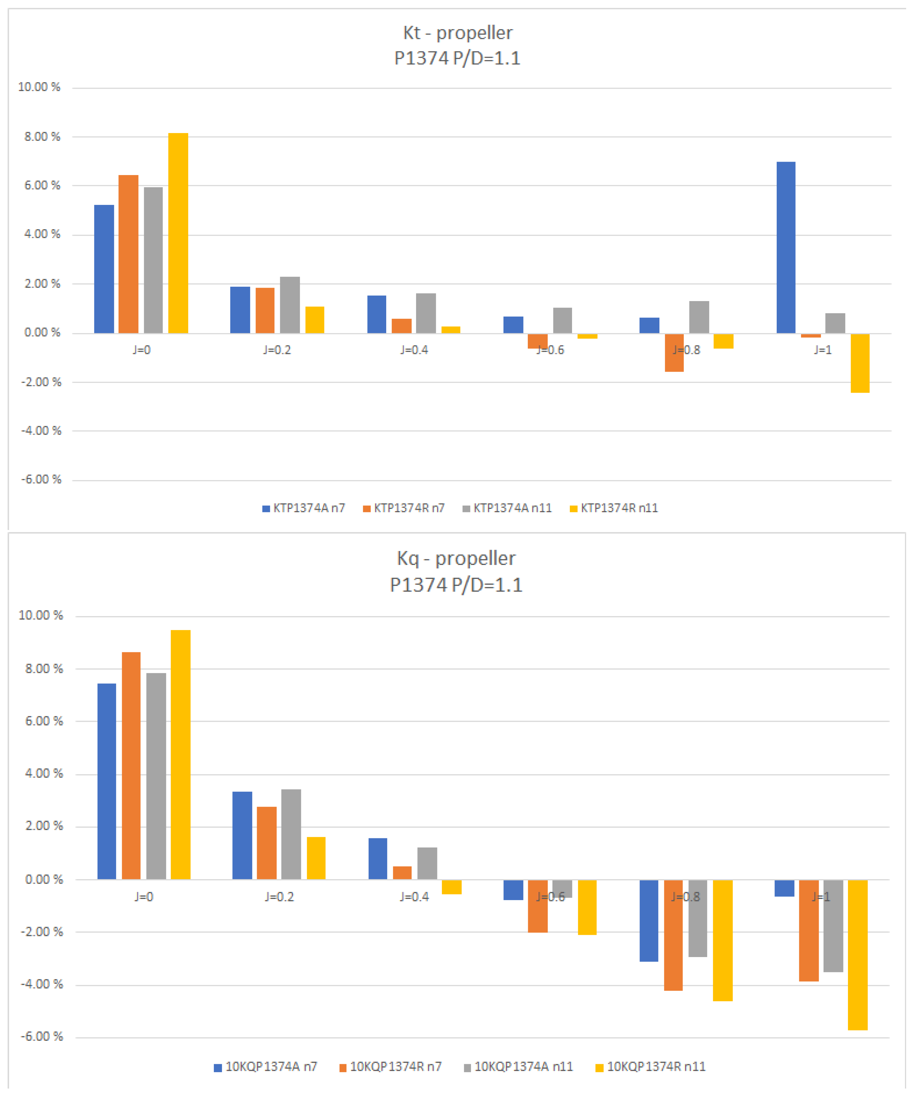

Figure 13.
Bend and twist of a typical blade section towards the tip: The top plot shows the same cylindrical section unloaded and loaded. The bottom picture shows the same sections once the bending is removed from the loaded blade so that the blade twist can be more easily seen.
Figure 13.
Bend and twist of a typical blade section towards the tip: The top plot shows the same cylindrical section unloaded and loaded. The bottom picture shows the same sections once the bending is removed from the loaded blade so that the blade twist can be more easily seen.

Figure 14.
Total displacement and twist of a section close to the blade root: The top plot shows the same cylindrical section unloaded and loaded. In the bottom picture, the procedure of removing the section bending is applied showing that, close to the blade root, the sections are warping rather than twisting.
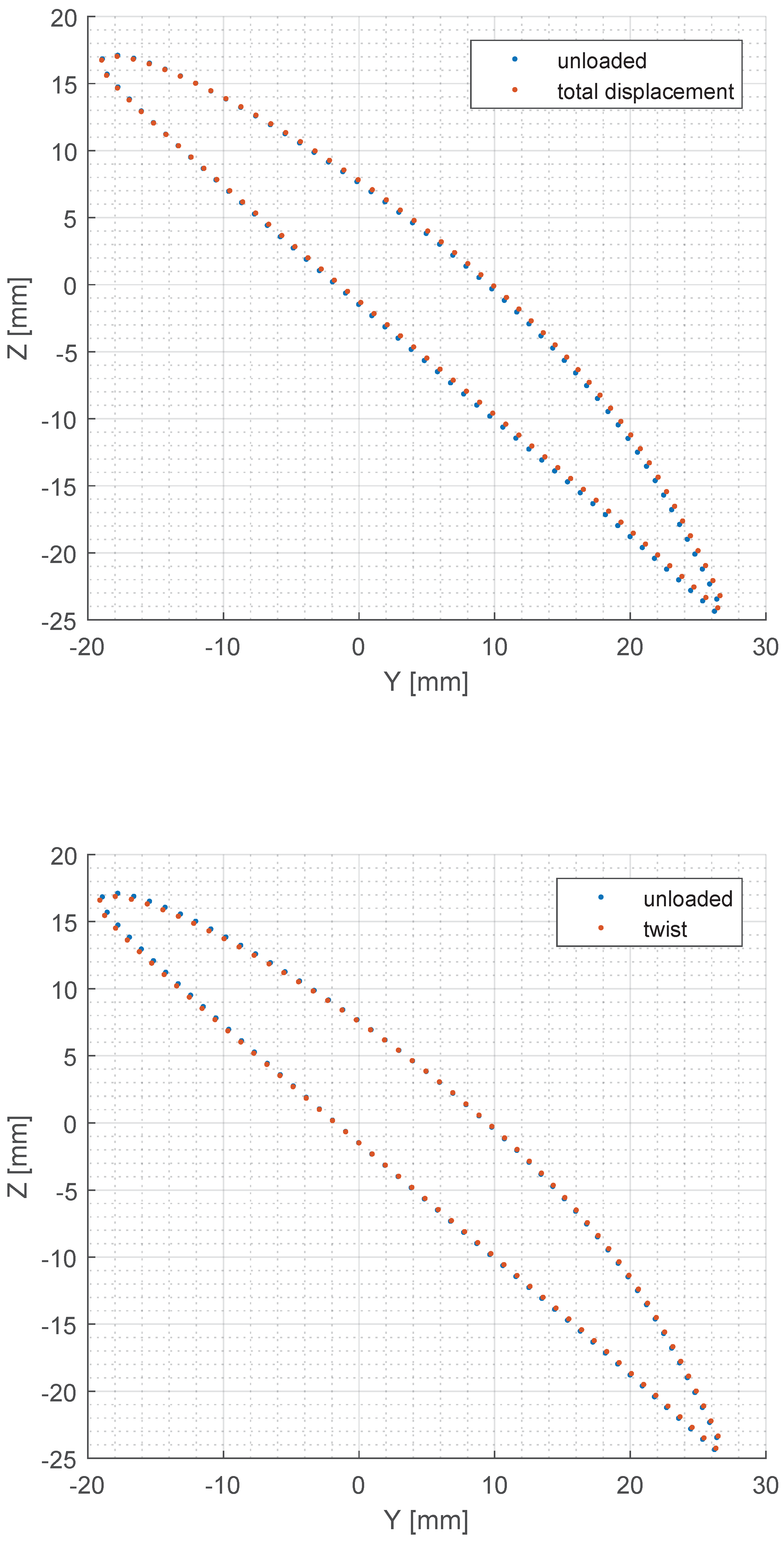
Figure 15.
Bending of the three different blade geometries at = 1.1 and 11 rps.

Figure 16.
Twist of the three different blade geometries at = 1.1 and 11 rps.
© 2020 by the authors. Licensee MDPI, Basel, Switzerland. This article is an open access article distributed under the terms and conditions of the Creative Commons Attribution (CC BY) license (http://creativecommons.org/licenses/by/4.0/).
Share and Cite
MDPI and ACS Style
Savio, L.; Sileo, L.; Kyrre Ås, S. A Comparison of Physical and Numerical Modeling of Homogenous Isotropic Propeller Blades. J. Mar. Sci. Eng. 2020, 8, 21. https://doi.org/10.3390/jmse8010021
AMA Style
Savio L, Sileo L, Kyrre Ås S. A Comparison of Physical and Numerical Modeling of Homogenous Isotropic Propeller Blades. Journal of Marine Science and Engineering. 2020; 8(1):21. https://doi.org/10.3390/jmse8010021
Chicago/Turabian StyleSavio, Luca, Lucia Sileo, and Sigmund Kyrre Ås. 2020. "A Comparison of Physical and Numerical Modeling of Homogenous Isotropic Propeller Blades" Journal of Marine Science and Engineering 8, no. 1: 21. https://doi.org/10.3390/jmse8010021
Note that from the first issue of 2016, this journal uses article numbers instead of page numbers. See further details here.