Development and Application of an Empirical Dune Growth Model for Evaluating Barrier Island Recovery from Storms


Abstract
:1. Introduction
2. Materials and Methods
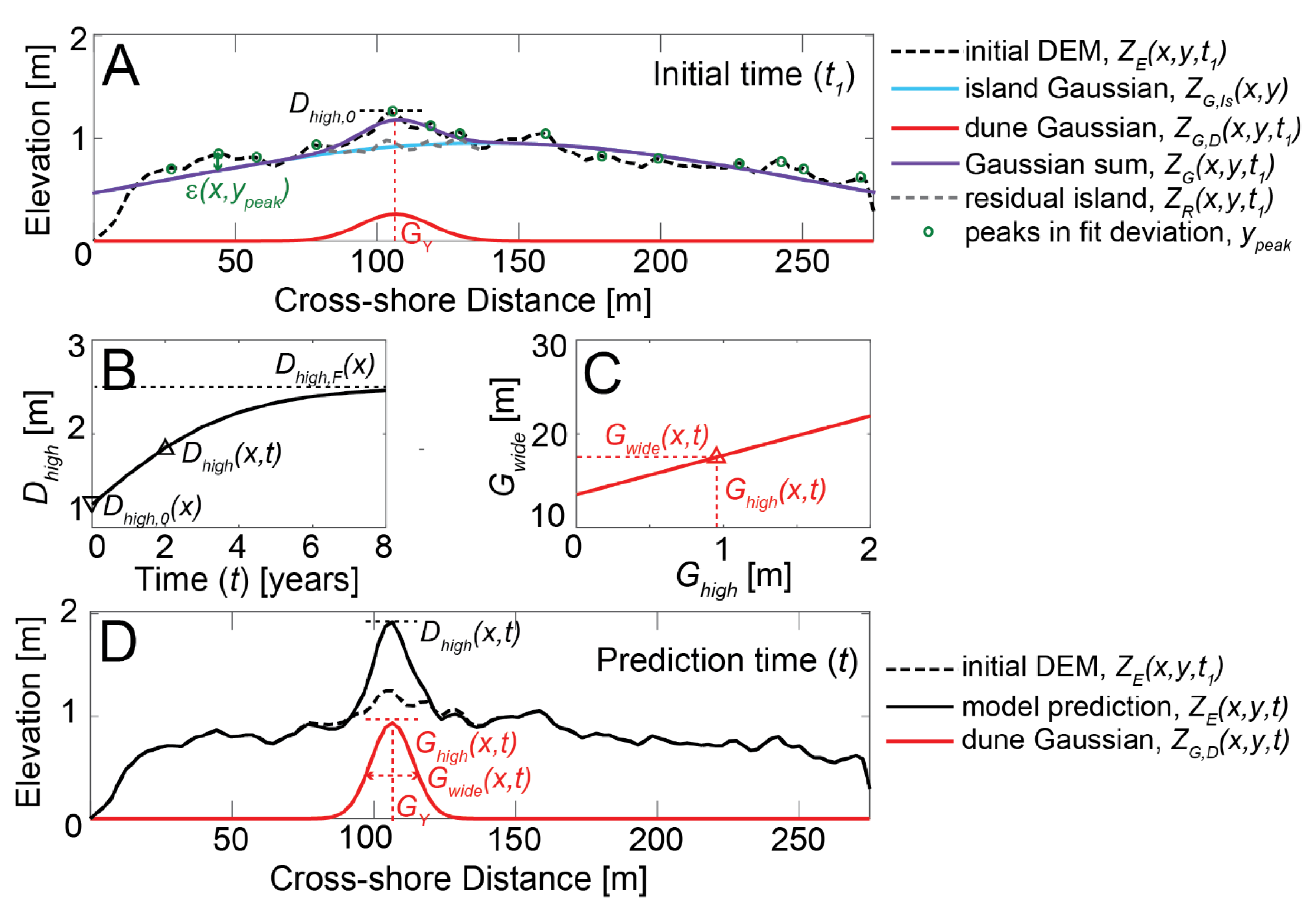
2.1. Empirical Dune Growth (EDGR) Model
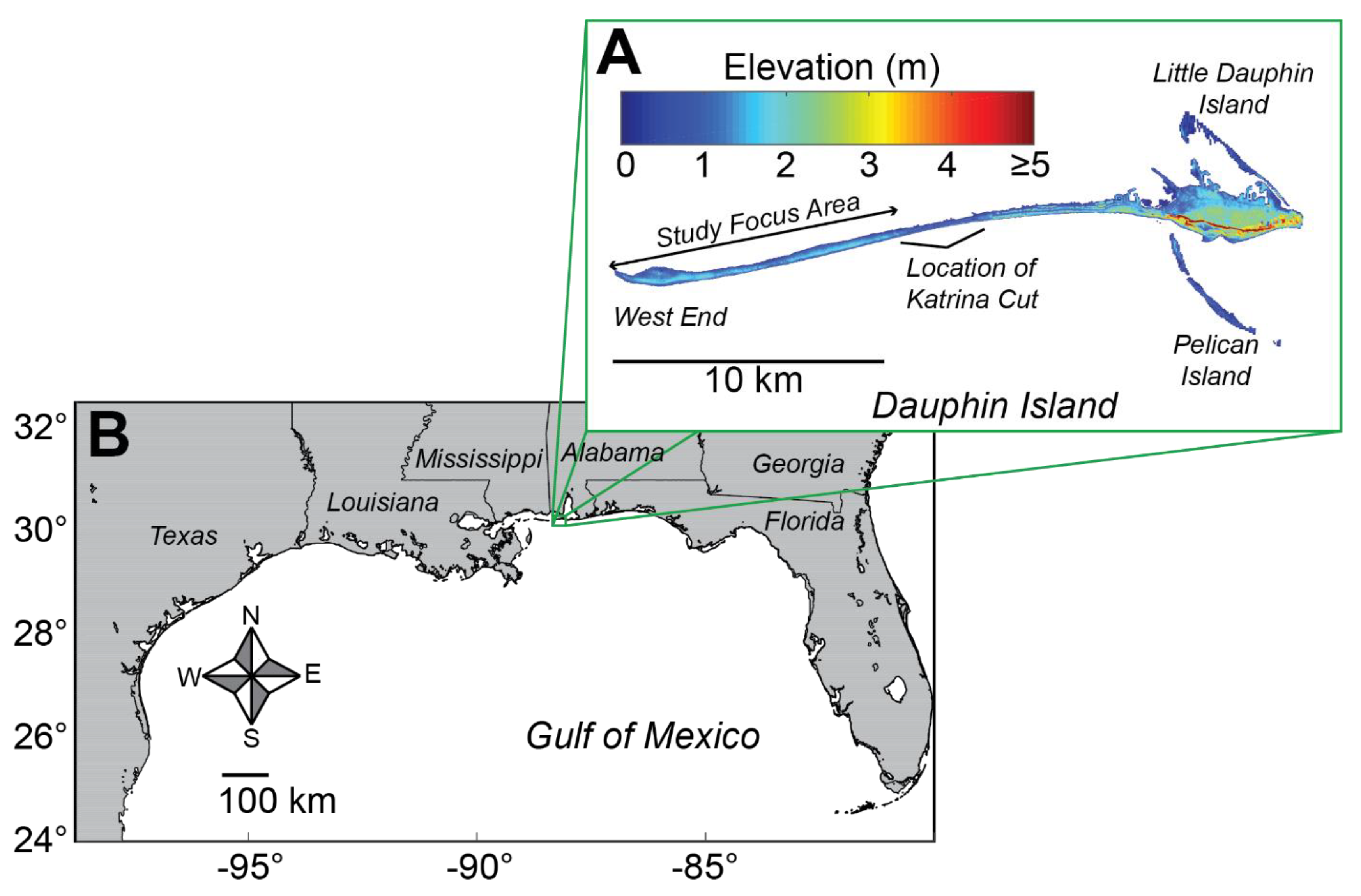
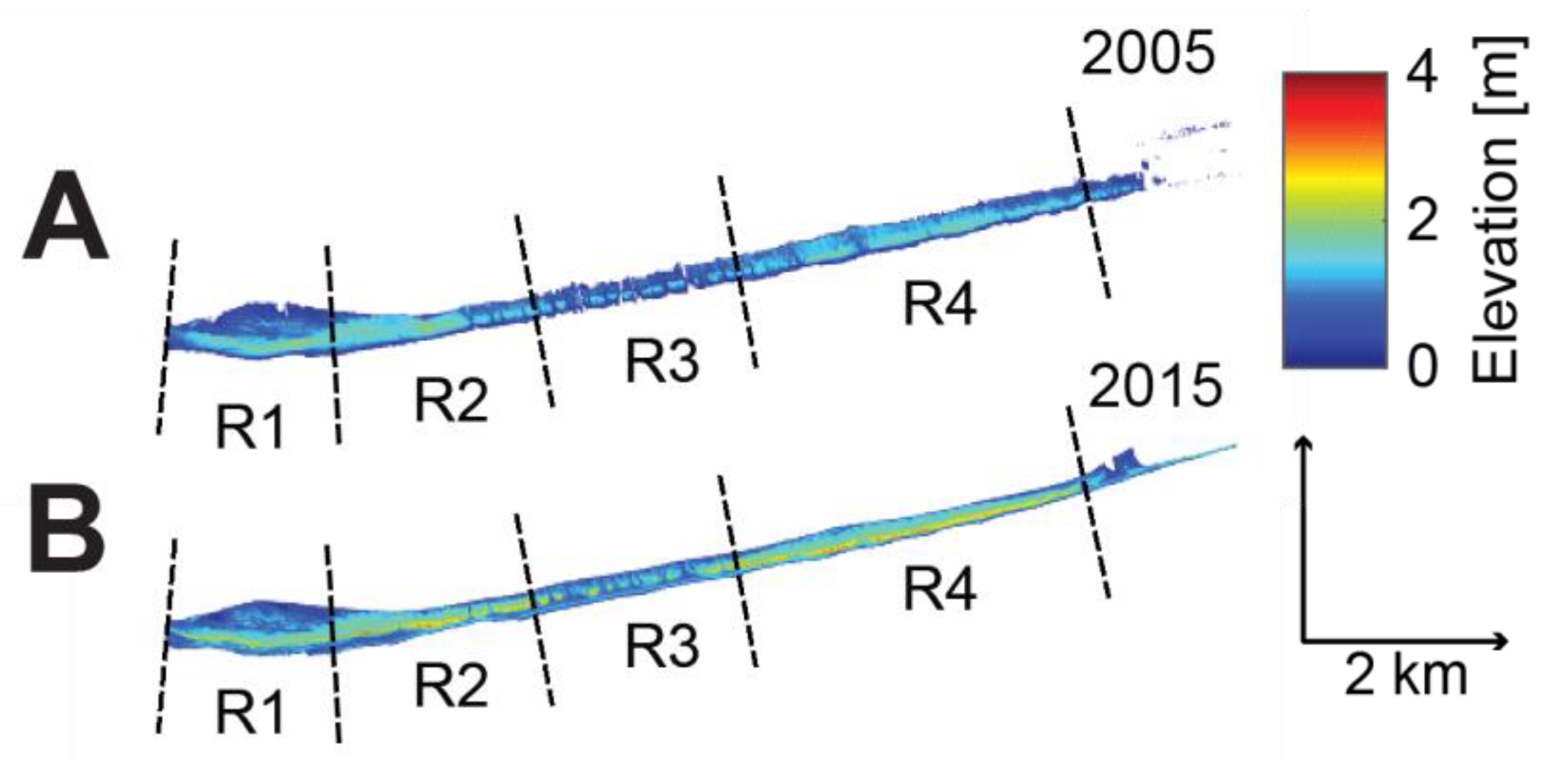
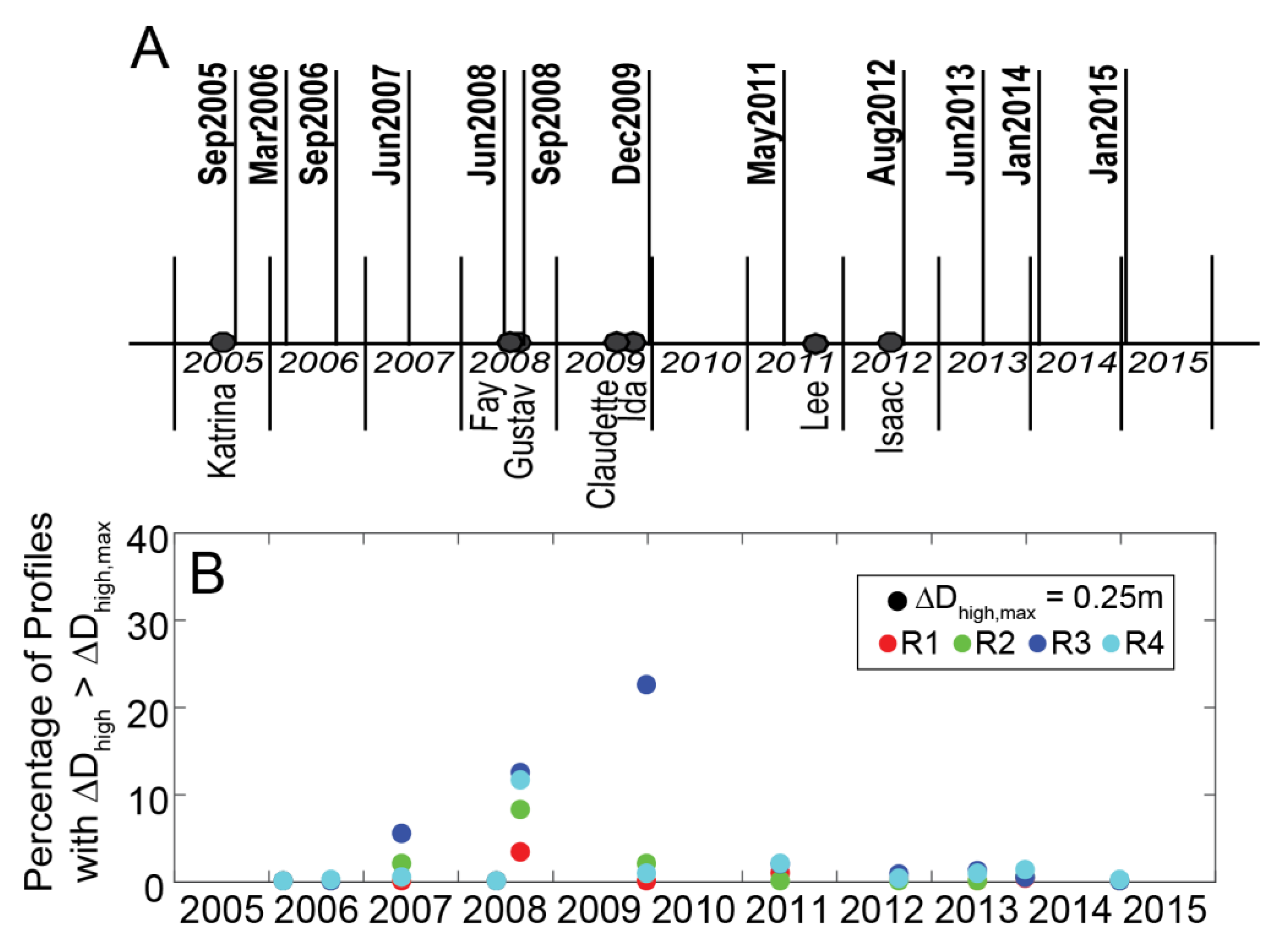
2.2. Study Site and Model Configuration
3. Results
3.1. Prescribed Terminal Dunes (Experiment E1)
3.2. Template Terminal Dunes (Experiments E2–E6)
4. Discussion
4.1. Dune Characterization
4.2. Dune Evolution
4.3. Broader Model Application
5. Conclusions
Author Contributions
Funding
Acknowledgments
Conflicts of Interest
Appendix A

| Region | R1 | R2 | R3 | R4 | ||||||||
|---|---|---|---|---|---|---|---|---|---|---|---|---|
| Statistic | RMSE (m) | Bias (m) | R2 (%) | RMSE (m) | Bias (m) | R2 (%) | RMSE (m) | Bias (m) | R2 (%) | RMSE (m) | Bias (m) | R2 (%) |
| L2005 | 61 | 50 | 0.17 | 59 | 36 | 0.39 | 43 | −7 | 0.02 | 25 | −6 | 0.24 |
| E1 | 0 | 0 | 1 | 0 | 0 | 1 | 0 | 0 | 1 | 0 | 0 | 1 |
| E2 | 36 ± 6 | −15 ± 10 | 0.06 ± 0.08 | 27 ± 4 | −8 ± 8 | 0.14 ± 0.14 | 27 ± 3 | 3 ± 8 | 0.18 ± 0.07 | 25 ± 3 | 7 ± 7 | 0.07 ± 0.06 |
| E3 | 35 ± 3 | −18 ± 1 | 0.05 ± 0.07 | 25 ± 2 | −10 ± 1 | 0.14 ± 0.08 | 23 ± 2 | 1 ± 1 | 0.21 ± 0.06 | 22 ± 1 | 5 ± 0 | 0.08 ± 0.06 |
| E4 | 41 ± 4 | −25 ± 5 | 0.04 ± 0.05 | 30 ± 3 | −17 ± 3 | 0.13 ± 0.13 | 25 ± 3 | −6 ± 3 | 0.19 ± 0.07 | 23 ± 3 | −2 ± 2 | 0.09 ± 0.10 |
| E5 | 0 1 | 0 1 | 1 1 | 0 1 | 0 1 | 1 1 | 0 1 | 01 | 1 1 | 01 | 0 1 | 1 1 |
| E6 | 0 1 | 0 1 | 1 1 | 0 1 | 0 1 | 1 1 | 0 1 | 0 1 | 1 1 | 0 1 | 0 1 | 1 1 |
| Region | R1 | R2 | R3 | R4 | ||||||||
|---|---|---|---|---|---|---|---|---|---|---|---|---|
| Statistic | RMSE (m) | Bias (m) | R2 (%) | RMSE (m) | Bias (m) | R2 (%) | RMSE (m) | Bias (m) | R2 (%) | RMSE (m) | Bias (m) | R2 (%) |
| L2005 | 0.69 | −0.52 | 0.11 | 0.96 | −0.79 | 0.18 | 0.81 | −0.54 | 0.16 | 0.95 | −0.82 | 0.21 |
| E1 | 0.18 | −0.02 | 0.85 | 0.21 | 0.07 | 0.89 | 0.28 | −0.06 | 0.84 | 0.18 | 0 | 0.89 |
| E2 | 0.53 ± 0.07 | 0.04 ± 0.19 | 0.28 ± 0.09 | 0.59 ± 0.09 | −0.18 ± 0.17 | 0.27 ± 0.11 | 0.74 ± 0.09 | 0.18 ± 0.14 | 0.24 ± 0.06 | 0.58 ± 0.07 | −0.16 ± 0.08 | 0.27 ± 0.12 |
| E3 | 0.61 ± 0.04 | −0.27 ± 0.04 | 0.17 ± 0.05 | 0.81 ± 0.04 | −0.54 ± 0.03 | 0.12 ± 0.05 | 0.67 ± 0.04 | −0.08 ± 0.04 | 0.19 ± 0.06 | 0.75 ± 0.03 | −0.48 ± 0.02 | 0.15 ± 0.04 |
| E4 | 0.50 ± 0.05 | 0.13 ± 0.09 | 0.35 ± 0.05 | 0.50 ± 0.05 | −0.10 ± 0.07 | 0.37 ± 0.09 | 0.74 ± 0.05 | 0.31 ± 0.06 | 0.28 ± 0.05 | 0.50 ± 0.04 | −0.05 ± 0.04 | 0.34 ± 0.07 |
| E5 | 0.53 ± 0.07 | 0.10 ± 0.19 | 0.24 ± 0.10 | 0.58 ± 0.08 | −0.13 ± 0.17 | 0.25 ± 0.11 | 0.69 ± 0.09 | 0.22 ± 0.14 | 0.33 ± 0.07 | 0.56 ± 0.07 | −0.11 ± 0.08 | 0.27 ± 0.12 |
| E6 | 0.52 ± 0.07 | 0.10 ± 0.19 | 0.25 ± 0.10 | 0.57 ± 0.08 | −0.14 ± 0.17 | 0.28 ± 0.11 | 0.57 ± 0.07 | 0.12 ± 0.12 | 0.48 ± 0.08 | 0.54 ± 0.07 | −0.12 ± 0.08 | 0.29 ± 0.11 |
References
- Sallenger, J. Storm impact scale for barrier islands. J. Coast. Res. 2000, 16, 890–895. [Google Scholar]
- Stockdon, H.F.; Sallenger, A.H.; Holman, R.A.; Howd, P.A. A simple model for the spatially-variable coastal response to hurricanes. Mar. Geol. 2007, 238, 1–20. [Google Scholar] [CrossRef]
- Long, J.W.; De Bakker, A.T.M.; Plant, N.G. Scaling coastal dune elevation changes across storm-impact regimes. Geophys. Res. Lett. 2014, 41, 2899–2906. [Google Scholar] [CrossRef] [Green Version]
- Larson, M.; Erikson, L.; Hanson, H. An analytical model to predict dune erosion due to wave impact. Coast. Eng. 2004, 51, 675–696. [Google Scholar] [CrossRef]
- Palmsten, M.L.; Holman, R.A. Laboratory investigation of dune erosion using stereo video. Coast. Eng. Proc. 2012, 60, 123–135. [Google Scholar] [CrossRef]
- Heijer, C.D.; Knipping, D.T.; Plant, N.G.; Vries, J.S.V.T.D.; Baart, F.; Van Gelder, P. Impact Assessment of Extreme Storm Events Using a Bayesian Network. Coast. Eng. Proc. 2012, 1. [Google Scholar] [CrossRef] [Green Version]
- Lentz, E.E.; Hapke, C.J.; Stockdon, H.F.; Hehre, R.E. Improving understanding of near-term barrier island evolution through multi-decadal assessment of morphologic change. Mar. Geol. 2013, 337, 125–139. [Google Scholar] [CrossRef] [Green Version]
- Plant, N.G.; Stockdon, H.F. Probabilistic prediction of barrier-island response to hurricanes. J. Geophys. Res. Space Phys. 2012, 117, 17. [Google Scholar] [CrossRef]
- Wilson, K.E.; Adams, P.N.; Hapke, C.J.; Lentz, E.E.; Brenner, O.T. Application of Bayesian Networks to hindcast barrier island morphodynamics. Coast. Eng. 2015, 102, 30–43. [Google Scholar] [CrossRef]
- Roelvink, J.A.; Reniers, A.; Van Dongeren, A.; Vries, J.V.T.D.; McCall, R.; Lescinski, J. Modelling storm impacts on beaches, dunes and barrier islands. Coast. Eng. 2009, 56, 1133–1152. [Google Scholar] [CrossRef]
- Houser, C.; Wernette, P.; Rentschlar, E.; Jones, H.; Hammond, B.; Trimble, S. Post-storm beach and dune recovery: Implications for barrier island resilience. Geomorphology 2015, 234, 54–63. [Google Scholar] [CrossRef]
- Keijsers, J.G.S.; Poortinga, A.; Riksen, M.J.P.M.; Maroulis, J. Spatio-Temporal Variability in Accretion and Erosion of Coastal Foredunes in the Netherlands: Regional Climate and Local Topography. PLoS ONE 2014, 9, e91115. [Google Scholar] [CrossRef] [Green Version]
- Dalyander, P.S.; Meyers, M.; Mattsson, B.J.; Steyer, G.; Godsey, E.; McDonald, J.; Byrnes, M.R.; Ford, M. Use of structured decision-making to explicitly incorporate environmental process understanding in management of coastal restoration projects: Case study on barrier islands of the northern Gulf of Mexico. J. Environ. Manag. 2016, 183, 497–509. [Google Scholar] [CrossRef] [Green Version]
- Luna, M.C.D.M.; Parteli, E.J.; Durán, O.; Herrmann, H.J. Model for the genesis of coastal dune fields with vegetation. Geomorphology 2011, 129, 215–224. [Google Scholar] [CrossRef]
- Jackson, N.L.; Nordstrom, K.F. Aeolian sediment transport and landforms in managed coastal systems: A review. Aeolian Res. 2011, 3, 181–196. [Google Scholar] [CrossRef]
- Psuty, N.P. Sediment budget and dune/beach interaction. J. Coast. Res. 1988, 3, 1–4. [Google Scholar]
- Psuty, N.P. Spatial Variation in Coastal Foredune Development. In Proceedings of the 3rd European Dune Congress, Galway, Ireland, 17–21 June 1992; pp. 3–13. [Google Scholar]
- Hesp, P.A. Surfzone, beach, and foredune interactions on the Australian SE coast. J. Coast. Res. 1988, 3, 15–25. [Google Scholar]
- Larson, M.; Palalane, J.; Hallin, C.; Hanson, H. Simulating cross-shore material exchange at decadal scale. Theory and model component validation. Coast. Eng. 2016, 116, 57–66. [Google Scholar] [CrossRef]
- Lorenzo-Trueba, J.; Ashton, A.D. Rollover, drowning, and discontinuous retreat: Distinct modes of barrier response to sea-level rise arising from a simple morphodynamic model. J. Geophys. Res. Earth Surf. 2014, 119, 779–801. [Google Scholar] [CrossRef] [Green Version]
- Bagnold, R.A. The movement of desert sand. Proc. R. Soc. Math Phys. Eng. Sci. 1936, 157, 594–620. [Google Scholar] [CrossRef]
- Sherman, D.J.; Jackson, D.W.; Namikas, S.L.; Wang, J. Wind-blown sand on beaches: An evaluation of models. Geomorphology 1998, 22, 113–133. [Google Scholar] [CrossRef]
- Davidson-Arnott, R.; Bauer, B. Aeolian sediment transport on a beach: Thresholds, intermittency, and high frequency variability. Geomorphology 2009, 105, 117–126. [Google Scholar] [CrossRef]
- Davidson-Arnott, R.G.; Law, M.N. Measurement and Prediction of Long-term Sediment Supply to Coastal Foredunes. J. Coast. Res. 1996, 12, 654–663. [Google Scholar]
- Delgado-Fernandez, I. A review of the application of the fetch effect to modelling sand supply to coastal foredunes. Aeolian Res. 2010, 2, 61–70. [Google Scholar] [CrossRef] [Green Version]
- Jackson, D.W.; Cooper, A. Beach fetch distance and aeolian sediment transport. Sedimentology 1999, 46, 517–522. [Google Scholar] [CrossRef]
- Davidson-Arnott, R.G.; MacQuarrie, K.; Aagaard, T. The effect of wind gusts, moisture content and fetch length on sand transport on a beach. Geomorphology 2005, 68, 115–129. [Google Scholar] [CrossRef]
- Bauer, B.O.; Davidson-Arnott, R.G.D. A general framework for modeling sediment supply to coastal dunes including wind angle, beach geometry, and fetch effects. Geomorphology 2003, 49, 89–108. [Google Scholar] [CrossRef]
- De Vries, S.; Arens, S.; De Schipper, M.A.; Ranasinghe, R. Aeolian sediment transport on a beach with a varying sediment supply. Aeolian Res. 2014, 15, 235–244. [Google Scholar] [CrossRef]
- De Vries, S.; Vries, J.V.T.D.; Van Rijn, L.; Arens, S.; Ranasinghe, R. Aeolian sediment transport in supply limited situations. Aeolian Res. 2014, 12, 75–85. [Google Scholar] [CrossRef]
- Gutierrez, B.T.; Plant, N.G.; Thieler, E.R. A Bayesian network to predict coastal vulnerability to sea level rise. J. Geophys. Res. Space Phys. 2011, 116, 1–15. [Google Scholar] [CrossRef] [Green Version]
- Da Silva, G.M.; Hesp, P.A. Coastline orientation, aeolian sediment transport and foredune and dunefield dynamics of Moçambique Beach, Southern Brazil. Geomorphology 2010, 120, 258–278. [Google Scholar] [CrossRef]
- Hesp, P.A.; Smyth, T.A.G. Surfzone-Beach-Dune interactions: Flow and Sediment Transport across the Intertidal Beach and Backshore. J. Coast. Res. 2016, 75, 8–12. [Google Scholar] [CrossRef] [Green Version]
- Jackson, N.L.; Nordstrom, K.F. Effects of Time-dependent Moisture Content of Surface Sediments on Aeolian Transport Rates Across a Beach, Wildwood, New Jersey, USA. Earth Surf. Process. Landf. 1997, 22, 611–621. [Google Scholar] [CrossRef]
- Zhang, W.; Schneider, R.; Kolb, J.; Teichmann, T.; Dudzinska-Nowak, J.; Harff, J.; Hanebuth, T.J. Land–sea interaction and morphogenesis of coastal foredunes—A modeling case study from the southern Baltic Sea coast. Coast. Eng. 2015, 99, 148–166. [Google Scholar] [CrossRef]
- Walker, I.J.; Davidson-Arnott, R.G.D.; Bauer, B.O.; Hesp, P.A.; Delgado-Fernandez, I.; Ollerhead, J.; Smyth, T.A. Scale-dependent perspectives on the geomorphology and evolution of beach-dune systems. Earth Sci. Rev. 2017, 171, 220–253. [Google Scholar] [CrossRef]
- Hoonhout, B.; De Vries, S. A process-based model for aeolian sediment transport and spatiotemporal varying sediment availability. J. Geophys. Res. Earth Surf. 2016, 121, 1555–1575. [Google Scholar] [CrossRef]
- Janssen, T. Aeolian Transport on a Beach: Testing the AeoLIS Aeolian Sediment Transport Model Against the Observed Recovery of Fire Island. Master’s Thesis, Delft University of Technology, Delft, The Netherlands, 2016. Available online: https://repository.tudelft.nl/islandora/object/uuid:79d1805e-4a90-404f-bece-c3801eed5d6f?collection=education (accessed on 30 November 2020).
- Hesp, P. Foredunes and blowouts: Initiation, geomorphology and dynamics. Geomorphology 2002, 48, 245–268. [Google Scholar] [CrossRef]
- Morton, R.A.; Paine, J.G.; Gibeaut, J.C. Stages and durations of post-storm beach recovery, southeastern Texas Coast, USA. J. Coast. Res. 1994, 10, 884–908. [Google Scholar]
- Short, A.D. Three Dimensional Beach-Stage Model. J. Geol. 1979, 87, 553–571. [Google Scholar] [CrossRef]
- Wright, L.; Short, A. Morphodynamic variability of surf zones and beaches: A synthesis. Mar. Geol. 1984, 56, 93–118. [Google Scholar] [CrossRef]
- Short, A.; Hesp, P. Wave, beach and dune interactions in southeastern Australia. Mar. Geol. 1982, 48, 259–284. [Google Scholar] [CrossRef]
- McLean, R.; Shen, J.-S. From Foreshore to Foredune: Foredune Development Over the Last 30 Years at Moruya Beach, New South Wales, Australia. J. Coast. Res. 2006, 221, 28–36. [Google Scholar] [CrossRef]
- Pender, D.; Karunarathna, H. A statistical-process based approach for modelling beach profile variability. Coast. Eng. 2013, 81, 19–29. [Google Scholar] [CrossRef] [Green Version]
- Nordstrom, K.F. Coastal Dunes. In Coastal Environments and Global Change; John Wiley and Sons: London, UK, 2015; pp. 178–193. [Google Scholar]
- Lalimi, F.Y.; Silvestri, S.; Moore, L.J.; Marani, M. Coupled topographic and vegetation patterns in coastal dunes: Remote sensing observations and ecomorphodynamic implications. J. Geophys. Res. Biogeosci. 2017, 122, 119–130. [Google Scholar] [CrossRef]
- Bitton, M.C.A.; Hesp, P.A. Vegetation dynamics on eroding to accreting beach-foredune systems, Florida panhandle. Earth Surf. Process. Landf. 2013, 38, 1472–1480. [Google Scholar] [CrossRef]
- Durán, O.; Moore, L.J. Vegetation controls on the maximum size of coastal dunes. Proc. Natl. Acad. Sci. USA 2013, 110, 17217–17222. [Google Scholar] [CrossRef] [Green Version]
- Zarnetske, P.L.; Ruggiero, P.; Seabloom, E.W.; Hacker, S.D. Coastal foredune evolution: The relative influence of vegetation and sand supply in the US Pacific Northwest. J. R. Soc. Interface 2015, 12, 20150017. [Google Scholar] [CrossRef] [Green Version]
- Nordstrom, K.F.; Jackson, N.L.; Korotky, K.H.; Puleo, J.A. Aeolian transport rates across raked and unraked beaches on a developed coast. Earth Surf. Process. Landf. 2010, 36, 779–789. [Google Scholar] [CrossRef]
- Zarnetske, P.L.; Hacker, S.D.; Seabloom, E.W.; Ruggiero, P.; Killian, J.R.; Maddux, T.B.; Cox, D. Biophysical feedback mediates effects of invasive grasses on coastal dune shape. Ecology 2012, 93, 1439–1450. [Google Scholar] [CrossRef] [PubMed]
- Van Puijenbroek, M.E.B.; Limpens, J.; De Groot, A.V.; Riksen, M.J.; Gleichman, M.; Slim, P.A.; Van Dobben, H.F.; Berendse, F. Embryo dune development drivers: Beach morphology, growing season precipitation, and storms. Earth Surf. Process. Landf. 2017, 42, 1733–1744. [Google Scholar] [CrossRef]
- Hugenholtz, C.H.; Wolfe, S.A. Biogeomorphic model of dunefield activation and stabilization on the northern Great Plains. Geomorphology 2005, 70, 53–70. [Google Scholar] [CrossRef]
- Lesser, G.; Roelvink, J.; Van Kester, J.; Stelling, G. Development and validation of a three-dimensional morphological model. Coast. Eng. 2004, 51, 883–915. [Google Scholar] [CrossRef]
- Mickey, R.C.; Long, J.W.; Dalyander, P.S.; Jenkins, R.L.; Thompson, D.M.; Passeri, D.L.; Plant, N.G. Development of a Modeling Framework for Predicting Decadal Barrier Island Evolution; US Geology Survey: Reston, VA, USA, 2020; p. 46.
- Mickey, R.C.; Godsey, E.; Dalyander, P.S.; Gonzalez, V.M.; Jenkins, R.L.; Long, J.W.; Thompson, D.M.; Plant, N.G. Application of Decadal Modeling Approach to Forecast Barrier Island Evolution, Dauphin Island, Alabama; US Geology Survey: Reston, VA, USA, 2020; p. 45.
- Passeri, D.L.; Dalyander, P.S.; Long, J.W.; Mickey, R.C.; Jenkins, R.L.; Thompson, D.M.; Plant, N.G.; Godsey, E.S.; Gonzalez, V.M. The Roles of Storminess and Sea Level Rise in Decadal Barrier Island Evolution. Geophys. Res. Lett. 2020, 47. [Google Scholar] [CrossRef]
- Mickey, R.C.; Dalyander, P.S.; McCall, R.; Passeri, D.L. Sensitivity of Storm Response to Antecedent Topography in the XBeach Model. J. Mar. Sci. Eng. 2020, 8, 829. [Google Scholar] [CrossRef]
- Brigham, E.O. The Fast Fourier Transform and Its Applications; Prentice Hall: Upper Saddle River, NJ, USA, 1998. [Google Scholar]
- Watkins, A.D. A Synthesis of Alabama Beach States and Nourishment Histories. Master’s Thesis, University of Alabama, Tuscaloosa, AL, USA, 2011. Available online: http://acumen.lib.ua.edu/u0015/0000001/0000723/u0015_0000001_0000723.pdf (accessed on 30 November 2020).
- Douglass, S.L. Beach erosion and deposition on Dauphin Island, Alabama, USA. J. Coast. Res. 1994, 10, 306–328. [Google Scholar]
- De Velasco, G.G.; Winant, C.D. Seasonal patterns of wind stress and wind stress curl over the Gulf of Mexico. J. Geophys. Res. 1996, 101, 18127–18140. [Google Scholar] [CrossRef]
- Dzwonkowski, B.; Park, K. Influence of wind stress and discharge on the mean and seasonal currents on the Alabama shelf of the northeastern Gulf of Mexico. J. Geophys. Res. 2010, 115, 12052. [Google Scholar] [CrossRef] [Green Version]
- Enwright, N.M.; Borchert, S.M.; Day, R.H.; Feher, L.C.; Osland, M.J.; Wang, L.; Wang, H. Barrier Island Habitat Map and Vegetation Survey—Dauphin Island, Alabama, 2015; US Geological Survey: Reston, VA, USA, 2017; p. 17.
- Thompson, D.M.; Dalyander, P.S.; Long, J.W.; Plant, N.G. Correction of Elevation Offsets in Multiple Co-Located Lidar Datasets; US Geological Survey: Reason, VA, USA, 2017.
- Morton, R.A. Historical Changes in the Mississippi-Alabama Barrier-Island Chain and the Roles of Extreme Storms, Sea Level, and Human Activities. J. Coast. Res. 2008, 246, 1587–1600. [Google Scholar] [CrossRef]
- Froede, C.R. The Impact that Hurricane Ivan (16 September 2004) Made across Dauphin Island, Alabama. J. Coast. Res. 2006, 223, 561–573. [Google Scholar] [CrossRef]
- Froede, C.R. Changes to Dauphin Island, Alabama, Brought about by Hurricane Katrina (29 August 2005). J. Coast. Res. 2008, 4, 110–117. [Google Scholar] [CrossRef]
- Morton, R.A.; Miller, T.L.; Moore, L.J. National Assessment of Shoreline Change: Part 1, Historical Shoreline Changes and Associated Coastal Land Loss Along the U.S. Gulf of Mexico; US Geological Survey: Reston, VA, USA, 2004. Available online: https://pubs.usgs.gov/of/2004/1043/ (accessed on 30 November 2020).
- Plant, N.G.; Freilich, M.H.; Holman, R.A. Role of morphologic feedback in surf zone sandbar response. J. Geophys. Res. Space Phys. 2001, 106, 973–989. [Google Scholar] [CrossRef] [Green Version]
- Christiansen, M.B.; Davidson-Arnott, R.G.D. Rates of Landward Sand Transport over the Foredune at Skallingen, Denmark and the Role of Dune Ramps. Geogr. Tidsskr. Dan. J. Geogr. 2004, 104, 31–43. [Google Scholar] [CrossRef]
- Houser, C. Synchronization of transport and supply in beach-dune interaction. Prog. Phys. Geogr. Earth Environ. 2009, 33, 733–746. [Google Scholar] [CrossRef]
- Gutierrez, B.T.; Plant, N.G.; Thieler, E.R.; Turecek, A.M. Using a Bayesian network to predict barrier island geomorphologic characteristics. J. Geophys. Res. Earth Surf. 2015, 120, 2452–2475. [Google Scholar] [CrossRef] [Green Version]
- Wolner, C.W.; Moore, L.J.; Young, D.R.; Brantley, S.T.; Bissett, S.N.; McBride, R.A. Ecomorphodynamic feedbacks and barrier island response to disturbance: Insights from the Virginia Barrier Islands, Mid-Atlantic Bight, USA. Geomorphology 2013, 199, 115–128. [Google Scholar] [CrossRef]
- McCall, R.; Vries, J.V.T.D.; Plant, N.; Van Dongeren, A.; Roelvink, J.; Thompson, D.; Reniers, A. Two-dimensional time dependent hurricane overwash and erosion modeling at Santa Rosa Island. Coast. Eng. 2010, 57, 668–683. [Google Scholar] [CrossRef]

| Parameter | Description |
|---|---|
| x | Longshore position |
| y | Cross-shore position |
| ZE(x,y,t1) | Measured cross-shore elevation profile at initial time, t1 |
| ZG(x,y,t1) | Gaussian decomposition of cross-shore profile at initial time, t1 |
| e(x,y) | Fit deviation (error) between ZE(x,y,t1) and ZG(x,y,t1) |
| ZG,n(x,y,t) | Gaussian curves representing the underlying island platform (ZG,Is(x,y,t)) and one or more dunes (ZG,D(x,y,t)), if present |
| ZR(x,y,t1) | Residual elevation of the cross-shore profile excluding the foredune (ZR(x,y,t1) = ZE(x,y,t1)–ZG,D(x,y,t1)). |
| ZE(x,y,t) | EDGR-predicted profile at time t, derived by adding the predicted foredune elevation to the residual profile (ZE(x,y,t) = ZG,D(x,y,t) + ZR(x,y,t1)). |
| Dhigh(x,t) | Total elevation of the foredune at time t, equivalent to the height of the Gaussian curve representing the foredune (Ghigh(x,t)) plus the height of the residual island at the foredune location (ZR(x,yD,t1)) |
| Dhigh, 0(x) | Initial height of the foredune |
| Dhigh,F(x) | Terminal height of the foredune |
| r | Foredune growth rate |
| Ghigh(x,t) | Height of the Gaussian curve representing the foredune at time t |
| Gwide(x,t) | Width of the Gaussian curve representing the foredune at time t |
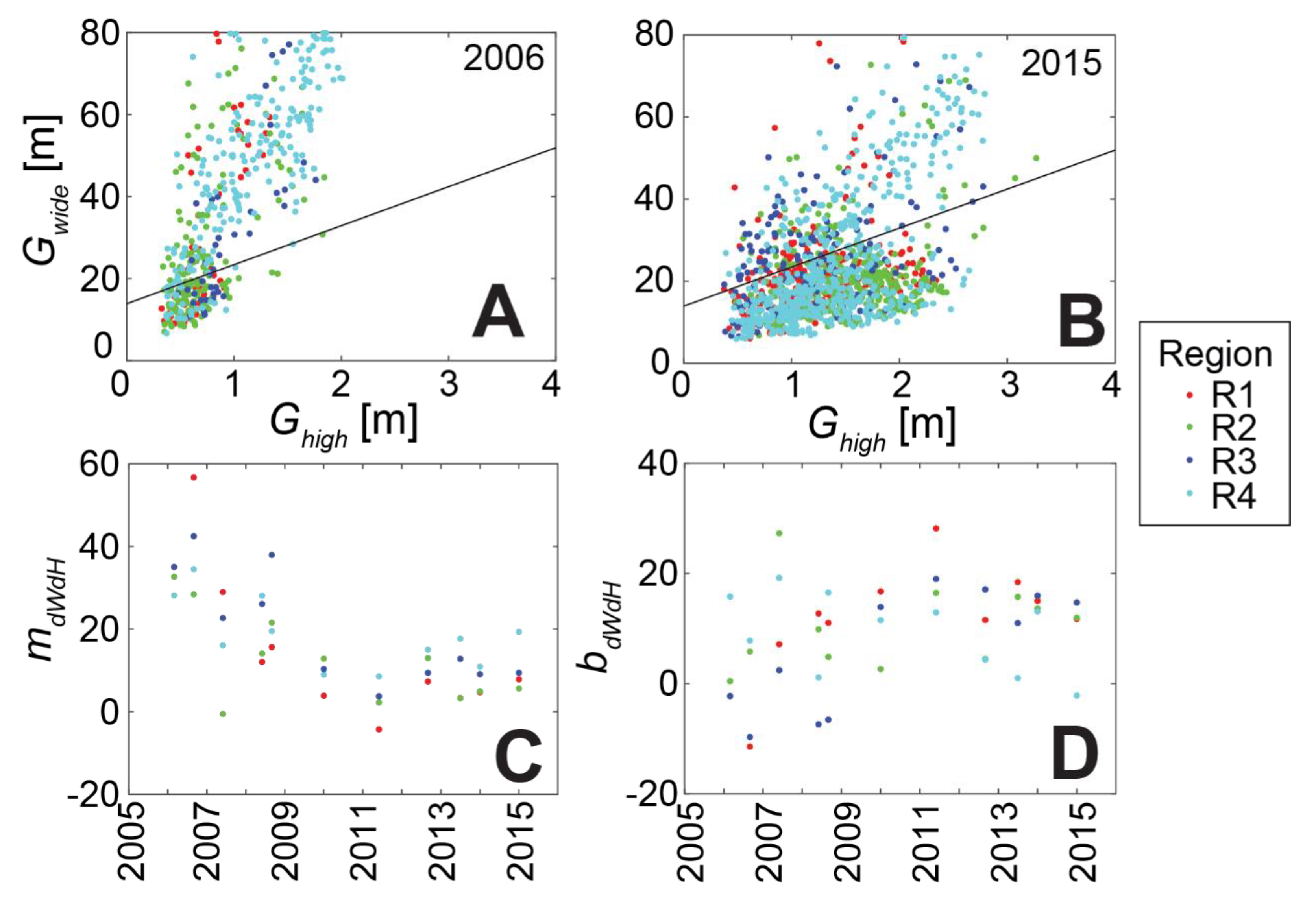
| mdWdH | Slope of the linear model used to predict Gwide(x,t) from Ghigh(x,t) |
| bdWdH | Y-intercept of the linear model used to predict Gwide(x,t) from Ghigh(x,t) |
| Dhigh,0 (m) | Dhigh,F (m) | r (m/yr) | DSL,0 (m) | mdWdH | bdWdH (m) | |
|---|---|---|---|---|---|---|
| R1 | 1.46 | 2.51 | 0.58 | 83 | 3.54 | 18.18 |
| R2 | 1.50 | 3.05 | 0.45 | 78 | 2.91 | 18.33 |
| R3 | 0.63 | 2.25 | 0.55 | 71 | 12.66 | 12.23 |
| R4 | 1.48 | 2.89 | 0.56 | 62 | 16.92 | 7.91 |
| R1–R4 | 1.29 | 2.75 | 0.53 | 71 | 9.50 | 13.90 |
| Experiment ID. | Dhigh,F (m) | DSL,0 | Realizations | Coupled to Lidar? | Threshold for Reset of Dhigh,0 |
|---|---|---|---|---|---|
| L2005 | n/a: no change model using 2005 lidar | ||||
| E1 | Prescribed from 2015 values | Prescribed from 2015 values | 1 | No | n/a |
| E2 | FFT with Regions 1–4 in template | FFT with Regions 1–4 in template | 100 | No | n/a |
| E3 | FFT with Region 3 in template | FFT with Region 3 in template | 100 | No | n/a |
| E4 | FFT with Region 4 in template | FFT with Region 4 in template | 100 | No | n/a |
| E5 | FFT with Regions 1–4 in template | Prescribed from 2015 values | 100 | No | n/a |
| E6 | FFT with Regions 1–4 in template | Prescribed from 2015 values | 100 | Yes | 0.25 m |
Publisher’s Note: MDPI stays neutral with regard to jurisdictional claims in published maps and institutional affiliations. |
© 2020 by the authors. Licensee MDPI, Basel, Switzerland. This article is an open access article distributed under the terms and conditions of the Creative Commons Attribution (CC BY) license (http://creativecommons.org/licenses/by/4.0/).
Share and Cite
Dalyander, P.S.; Mickey, R.C.; Passeri, D.L.; Plant, N.G. Development and Application of an Empirical Dune Growth Model for Evaluating Barrier Island Recovery from Storms. J. Mar. Sci. Eng. 2020, 8, 977. https://doi.org/10.3390/jmse8120977
Dalyander PS, Mickey RC, Passeri DL, Plant NG. Development and Application of an Empirical Dune Growth Model for Evaluating Barrier Island Recovery from Storms. Journal of Marine Science and Engineering. 2020; 8(12):977. https://doi.org/10.3390/jmse8120977
Chicago/Turabian StyleDalyander, P. Soupy, Rangley C. Mickey, Davina L. Passeri, and Nathaniel G. Plant. 2020. "Development and Application of an Empirical Dune Growth Model for Evaluating Barrier Island Recovery from Storms" Journal of Marine Science and Engineering 8, no. 12: 977. https://doi.org/10.3390/jmse8120977