Development of a Position Measuring Device of a Deep-Sea Pipeline Based on Flange Center Positioning

1
College of Mechanical and Electrical Engineering, Harbin Engineering University, Harbin 150001, China
2
School of Mechanical Engineering, Hebei University of Technology, Tianjin 300401, China
*
Author to whom correspondence should be addressed.
J. Mar. Sci. Eng. 2020, 8(2), 86; https://doi.org/10.3390/jmse8020086
Submission received: 15 December 2019
/
Revised: 7 January 2020
/
Accepted: 27 January 2020
/
Published: 1 February 2020
(This article belongs to the Special Issue Advances in Oceanic and Mechatronic Systems Engineering)
Abstract
:A deep-sea pipeline position and attitude-measuring device based on pipeline outer circle positioning can measure the spatial relative positions of the end faces of two oil pipelines in the deep sea. This device can provide the necessary data to make a transition pipeline connecting two sections of oil pipelines together. However, after analyzing the data measured by this device, it is found that the measurement data has a large error because the error transmission coefficient of the measurement value is too large. In order to reduce the error transfer coefficient, a new measuring device for measuring the posture of deep-sea pipelines by a tensioning rope was proposed. Unlike previous measuring devices, this measuring device is based on the positioning of the flange center of the pipe instead of the pin on the outer circle of the pipe. With the comparison of positioning methods between fixing in the center of flange and fixing the outer wall of pipeline, the former can reduce the transition matrix in the process of solving the relative position of the two pipes, and then reduce the magnification of the measurement sensor error. It also reduces two measurement parameters. The solving formula of the position and attitude of the measuring device based on the outer circle positioning of the pipeline is analyzed. It is proved that the error transmission coefficient of the measuring device based on the flange center positioning is smaller. Experiments show that compared with the positioning method based on the outer circle of the pipe, the positioning method based on the flange center has a higher accuracy.
1. Introduction
The ocean is rich in oil resources below 500 meters, and the transportation of oil from the deep sea to the land requires the use of oil pipelines in the deep sea [1,2]. In order to incorporate the pipeline of the new oilfield into the already laid submarine pipeline network, it is necessary to connect the two fixed-point pipelines together on the seabed [3,4]. At present, the main method of connecting deep-sea pipeline is to connect the two ends of the prepared transition pipeline to the oil outlet of the old pipeline and the oil inlet of the new pipeline [5]. The transition ducts that perfectly match the two sections of the pipeline need to accurately measure the relative position of the new and old pipelines. Therefore, deep-sea exploration equipment and technology have become hotspots in the international marine engineering community [6,7].
The location measurement of submarine pipelines mainly includes the following methods: underwater acoustic measurement, satellite positioning, and rope measurement [8]. Acoustic measurement is used by most underwater measurement operations. However, the underwater acoustic measurement system requires a large amount of equipment, and the installation work takes a long time. It is generally used for large-area mapping and geological exploration of seabed topography, and is rarely used in the measurement of underwater pipeline poses [9,10]. Satellite positioning technology is applied to a variety of underwater positioning tasks. For example, a measurement system consisting of underwater GPS and a single beam measuring instrument can effectively solve underwater high-precision positioning problems [11,12]. Drawstring measurements include traditional tensioning rope measurements and intelligent drawstring measurements. A diver carrying a measuring tool under water carries out the traditional tensioning rope measurement method [13]. The drawstring intelligent measurement method is suitable for a deep water environment, and it has the characteristics of high measurement accuracy and real-time dynamic measurement [14]. For example, the unmanned drawstring system developed by NGI of Norway, which is not limited by water depth, has a length accuracy of ±10 cm and an angular accuracy of ±0.5° [15]. Professor Wang Liquan of Harbin Engineering University in China proposed a deep-sea measurement system on the pipeline attitude. Its maximum working water depth is 1500 m, which can achieve a measurement accuracy of ±50 mm and ±1° within a 5 m working range [16]. In addition to the above methods, multi-beam sounding technology, inertial navigation measurement system, and side scan sonar are more and more used in the positioning and detection of underwater pipelines [17,18].
The article mainly studies the intelligent measurement method of the drawstring. By analyzing the error of the measuring device based on the outer circle positioning of the pipeline, it is determined that the existing measuring device can be optimized to improve the accuracy. Based on this, a cable-measuring device based on the center point of the flange was designed, its mathematical model was solved, and the error transfer coefficient was analyzed.
2. Measurement System and Experimental Method Based on Pipeline Circular Positioning
2.1. Composition of the Measurement System
On the working boat, the staff on board sends one instruction to the lower position machine of the ROV (Remote Operated Vehicle) through the umbilical cable, so that the ROV helps the measuring device to obtain the variable parameters for calculating the relative position of the two pipeline spaces, and then transmits the measurement data to the upper computer for calculation. The measuring system measures the rocking angle of the measuring device I and the measuring device II with respect to the absolute vertical plane and the tilting pitch angle with the absolute horizontal plane by means of an orthogonal inclination sensor on the measuring device. There are two magnetically coupled encoders on each measuring device for obtaining the horizontal and vertical corners of the projecting arm of the measuring device. In addition to this, the measuring device II has one more rope length-detecting device than the measuring device I connected to the magnetron cable winch for detecting the distance between the two measuring devices.
The deep-sea pipeline position and attitude measuring device based on the outer circle positioning of the pipeline mainly includes the measuring device I, the measuring device II, the base I, the base II, the drawstring, and the drawstring winch, as shown in Figure 1.
The orthogonal inclination sensor and the encoder mounted on the measuring device are connected to the positioning base. The positioning base I and the base II have the same structure, and they are positioning platforms for connecting the measuring device to the pipe.
2.2. Method for Measuring the Relative Position of Two Pipes
2.2.1. Mathematical Model and Solution Formula of the Measuring Device Based on the Outer Circle Positioning of the Pipeline
Figure 2 is the mathematical model I of the deep-sea pipeline position and orientation-measuring device based on pipeline outer circle positioning. Pr and Pb are the center points of the end faces of pipe I and pipe II, respectively. The pull-out points A and B of the tensioning rope are parallel planes of the two flange end faces, which are used as reference planes of the respective measuring devices, and the centerlines of the pipes are intersected at Or and O4, respectively. With Or and O4 as the origin, absolute coordinate systems ΩR and Ω4 are established, respectively, and the z-axis of these two coordinate systems are in the same direction. Set the reference coordinate system Ω1 with Or as the origin of the pipe centerline as the y-axis. The reference coordinate system Ω2 is obtained by positively translating Ω1 along its z-axis by R1. Rotate Ω2 around the z-axis until the x-axis coincides with the projection in plane A to establish the reference coordinate system Ω3. Create the reference coordinate system Ω5 with reference to Ω1.
Reference [16] solves the mathematical model I. Equation (1) is the calculation formula for the distance parameter and angle parameter between two pipes. In this way, the host computer can use this algorithm and the data measured by the sensor to calculate the relative distance between the centers and the relative angle of the two pipe end faces.
where PRPbx, PRPby, and PRPbz are the projection values of the vectors of the two pipeline centers in the X-axis, Y-axis, and Z-axis directions of the absolute coordinate system ΩR. ξx1, ξy1, and ξz1 are the angles formed by the axis of pipe II and the X, Y, and Z axes of the absolute coordinate system ΩR. αr and αb are the angles between the x-axis of the orthogonal tilt sensor of measurement device I and measurement device II and the absolute horizontal plane. βr and βb are the measurement device I and the measurement device, respectively. The angle is between the Y-axis of the orthogonal tilt sensor of the II and the absolute horizontal plane. γr and γb are the horizontal swing angles of the measuring rope in the reference coordinate system Ω1 and the reference coordinate system Ω2, respectively. Ra and Rb are the distance from the extension point of the tensioning rope to the mounting base I and the mounting base II, respectively. ea and eb are the distance between the mounting base I and the end face of pipe I and pipe II, respectively. L is the distance between the pullout points A and B. According to reference 16, L can be obtained by Equation (2).
where: S = sin (); C = cos (); T = tan (). l is the actual length of the tensioning rope. c is the relative height of the two measuring devices. Sr is the measuring length of the tensioning rope. θr and θb are the pitching angles of the tensioning rope in the reference coordinate system Ω1 and the reference coordinate system Ω2, respectively.
2.2.2. Measurement Test
The measurement experiment is mainly performed to compare the experimental data obtained by the measuring device with the actual relative position of the space of the two pipes in the case of simulating two pipes in different postures. The measurement experiment should be divided into the following steps.
(1) In the pipeline pose measurement experiment based on the outer circle positioning of the pipeline, it is first necessary to initialize the measuring device. That is, the position of pipe II is adjusted to ensure that the end faces of the two pipe flanges are parallel, and the pipe axes are coincident, as shown in Figure 3. Record the initial values of each sensor at this time. In addition to this, it is also necessary to measure the length of the two take-off points of the drawstring on the measuring device I and the measuring device II to the two pipe axes and to the horizontal distance to the end faces of the two pipes.
(2) After initialization, we will move pipe II to the next position and adjust the pitch angle and swing angle of pipe I, and then manipulate the magnetic power winch to tension the rope. At this time, the lower computer will obtain the data of each sensor and transmit it to the upper computer through the signal line. Next, the distance and angle of the flange center of pipe I and pipe II are measured by a laser range finder and an angle measuring instrument as reference values, and pipe II is moved to the next position to measure a plurality of sets of data.
(3) The measurement experiment based on the positioning of the outer circle of the pipeline uses a laser rangefinder to adjust the distance between the two pipeline centers to 2 m, 3 m, 4 m, 5 m, 6 m, and 7 m, and the angle measuring instrument is used to adjust the angles parameters ξx1, ξy1, and ξz1 formed by the axis of pipe II and the X, Y, and Z axes of the absolute coordinate system ΩR. It corresponds to the actual value in Table 1. Then the host computer calculates the angle parameters ξx1, ξy1, and ξz1 and the length parameters PRPbx, PRPby, and PRPbz, which are the projection values of the vectors of the two pipeline centers in the X-axis, Y-axis, and Z-axis directions of the absolute coordinate system ΩR. It corresponds to the measurements in Table 1.
2.3. Error Analysis
Since the measurements used to solve the mathematical model I are directly measured, the deterministic error propagation rate of the measurement system based on the outer circle positioning of the pipeline is
where: E(xi) is the deterministic error of each measurement and is the error transfer coefficient of the corresponding measurement; E(y) is the sum of the errors of each measurement. The error value of the orthogonal inclination sensor is ±0.1°. The value of the error transfer coefficient of some measurements calculated by Equation (3) is large, which causes the error of the sensor to be amplified. This may be because the number of transition matrices based on the mathematical model I is large, resulting in an increase in the magnification of the error transfer coefficient. Therefore, optimizing the structure of the measuring device can reduce the number of transition matrices in the solution process and improve the measurement accuracy.
3. Design of the Measuring Device Based on Flange Center Positioning
3.1. Overall Design
If the take-off point of the drawstring between the two measuring devices is on the axis of the pipe, the number of transition matrices can be reduced, and since the two measurement parameters Ra and Rb are no longer needed, the errors caused to the measurement system are eliminated. The measuring device is positioned using the outer end face of the flange so that the take-up point of the drawstring is on the axis of the pipe. Considering that the flange is more resistant to corrosion than the pipe, it can avoid installation errors introduced by pipe corrosion [19]. Therefore, a pipe position measuring device based on flange positioning is proposed, and its schematic diagram is shown in Figure 4.
The measuring device based on flange center positioning secures flange and electric drive three-jaw chuck, and it is positioned and mounted by the three-jaw chuck. This type of structure can better meet the alignment accuracy requirements of the measuring device.
The orthogonal tilt sensor was fixed in the three-jaw chuck. The angle measuring mechanism was fixed on the other side of the flange, consisting of a horizontal axis and a vertical axis that were centered and intersected at one point, which was also the take-up point of the drawstring on the axis of the pipe. The measuring device II has one more rope length detecting device located between the angle measuring mechanism and the flange.
3.2. Building and Solving the Mathematical Model of the Deep-Sea Pipeline Pose Measurement Device Based on Flange Positioning
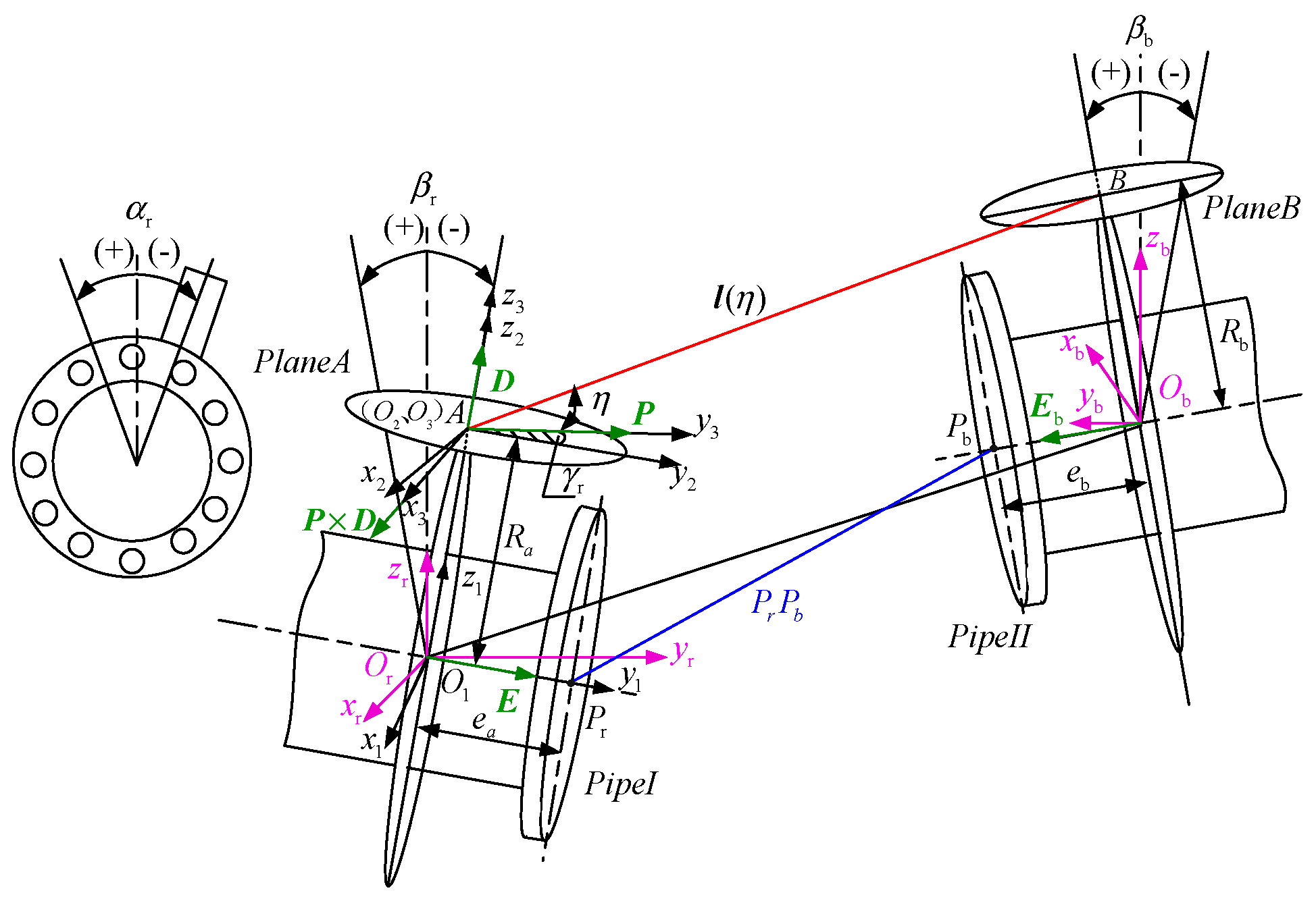
The mathematical model II for establishing the deep-sea pipeline pose measurement device based on flange positioning is shown in Figure 5. Then, we analyzed this mathematical model II in order to solve the angles parameters ξx2, ξy2, and ξz2 formed by the axis of pipe II and the X, Y, and Z axes of the absolute coordinate system ΩR and the length parameters ORObx, OROby, and ORObz, which are the projection values of the vectors of the two pipeline centers in the X-axis, Y-axis, and Z-axis directions of the absolute coordinate system ΩR. All subsequent formulas are based on this mathematical model II.
In the mathematical model II, Or and Ob are the center points of the end faces of pipe I and pipe II, respectively. The two flange end faces correspond to the plane C and the plane D, respectively, and the lead point A and the lead point B of the over-pull line are respectively made to plane A and plane B parallel to the flange end faces. The central axis of pipe I and the planes A and C intersect the points A and Or, respectively, and the central axis of the pipe of pipe II and the planes B and D intersect at points B and Ob, respectively. We can establish the absolute coordinate system ΩR with Or as the origin. The coordinate system ΩR is rotated about the x-axis and the y-axis to βr and αr to establish the reference coordinate system Ω1. βr and αr are the rocking angle of the measuring device I with respect to the pipe axis and the pitch angle of the absolute horizontal plane e, respectively. The absolute coordinate system Ωb and the reference coordinate system Ω3 are established. γr and θr are the horizontal swing angle and the pitch angle of the tensioning rope in the reference coordinate system Ω1, respectively. Similarly, αb, βb, γb, and θb can be expressed, and Sr is the measuring length of the tensioning rope.
For the measuring device I, there are rotation operators and between the coordinate systems Ω1 and ΩR, as shown in Equation (4). In the following Equations, S = sin (); C = cos (); T = tan ().
Therefore, the homogeneous transformation matrix between the coordinate systems Ω1 and ΩR is calculated by the Equation (5).
The unit vectors and are introduced in the coordinate system Ω1, and the coordinates of and are the unit vectors and in the absolute coordinate system ΩR, respectively. They are calculated by the Equation (6).
The coordinate system Ω1 is determined to be (,,) according to the unit vectors and . Equation (7) is the coordinate of in the coordinate system Ω1.
is the unit vector of and is projected as in the coordinate system Ω1 horizontal plane. Taking the vector along the direction establishes the coordinate system Ω2(,,). In Ω2, the coordinate of is . There is a rotation operator between the coordinate system Ω2 and Ω1, and the corresponding homogeneous transformation matrix is Equation (8).
Therefore, the transformation matrix between coordinate system Ω2 and coordinate system ΩR can be calculated by the Equation (9).
is the coordinates of in the absolute coordinate system ΩR. can be calculated by Equation (10).
Let be the angle between and plane A. Then the coordinate , which is the unit vector in the absolute coordinate system ΩR, can be calculated by Equation (11):
Let a be the projection length of the distance L between the pull-out points A and B in the Z-axis direction of the absolute coordinate system ΩR, which is a = c/L. The values of c and L can be solved by Equation (2). Substituting a for the Equation (11) to solve obtains Equation (12).
is the coordinate of the vector in the coordinate system ΩR. is the coordinate of the vector in the coordinate system Ωb. can be calculated by Equation (13) according to the mathematical model II.
Substituting into Equation (14) can calculate . Similarly, can be calculated by Equation (15).
The coordinates of and are the two bases in space. Introducing the transition matrix P and the transition angle Δp. The transition matrix P is calculated by Equation (16). The transition angle Δp is solved by the Equation (14) to the Equation (16), and Equation (17) is result of the transition angle Δp.
The transition matrix PT that makes the coordinate system Ωb to ΩR can be solved by the Equation (16) and the Equation (17). Since and are equal to the vertical distance from the projecting point of the tensioning rope to the end face of the flange in the two measuring devices, and can be calculated by Equation (18) according to the design size of measuring device.
where: m1 and m2 correspond to the vertical distances from the point A and the point B of the measuring device I and the measuring device II to the end faces of the flange, respectively.
From the Equation (7) and the Equation (10), the length parameters ORObx, OROby, and ORObz, which are the projection values of the vectors of the two pipeline centers in the X-axis, Y-axis, and Z-axis directions of the absolute coordinate system ΩR, can be calculated by Equation (19).
Establish a reference coordinate system Ωr as shown in Figure 6, and there is a rotation operator between the coordinate system ΩR and Ωr. In Figure 6, F1 and F2 correspond to O1 and O2 in mathematical model II, respectively. Let the unit vector of the central axis of pipe I be , and is the coordinate of in the coordinate system ΩR. Let the unit vector of the central axis of pipe II be , and is the coordinate of in the coordinate system Ωb. is the coordinate of the in the coordinate system ΩR, which is solved by Equation (20). Let . , which is the coordinate of in the coordinate system Ωr, is solved by Equation (21).
Similarly, which is the coordinate of in the coordinate system Ωr is solved by Equation (22).
The angle parameters ξx2, ξy2, and ξz2 can be calculated according to the Equation (19) and the Equation (20), as shown in Equation (23).
3.3. Analysis of Error Transfer Coefficient
Since the mathematical model II based on the flange center positioning compared to the measuring device based on the outer circle positioning of the pipe removes the parameters Ra and Rb, the error transfer coefficient analysis is performed based on the mathematical model I of the measuring system based on the outer circle positioning of the pipe. From Equation (24), Equation (25), and Equation (26), the error transfer coefficients Ci, Ni, Mi of the length parameters O1O2x, O1O2y, O1O2z related to the parameters Ra and Rb can be calculated.
As shown in Equation (24), the coefficients C1, N1, M1, N3, and M3 are affected by the parameters Ra, ea, and L. Ignoring the effect of ea on N3, the coefficient C1 is taken as an example to show the variation of the relative parameters Ra and L of C12 as shown in Figure 7. Figure 7 (a) corresponds to the same positive and negative αr and γr, and Figure 7 (b) corresponds to the difference between αr and γr. It can be seen from the figure that C1 is mainly affected by the parameter L and it is proportional to L. The parameter Ra has little effect on C12. The relative curves of the relative parameters Ra and L of N12, M12, N32, and M32 are similar to those of C12.
As shown in Equation (25), the coefficients C2, N2, and M2 are affected by the parameter Rb. Since the values of αb and βb are usually small and N2 is proportional to Rb, the value of C2 can be decreased by decreasing the value of Rb.
As shown in Equation (26), the coefficients C3, N4, M4 are affected by the parameters eb and Rb. The change surface of C32 with eb and Rb as variables is shown in Figure 8.
Figure 8a corresponds to βb less than 0, and Figure 8b corresponds to βb greater than 0. As can be seen from the figure, the parameter eb has less influence on C32, and C32 is proportional to eb. The maximum value is more than eight times the minimum value. The relative curves of N42 and M42 relative to parameters eb and Rb are similar to those of C32.
In summary, when the error transfer coefficient is related to the parameter L, it is mainly affected by the parameter L, and has little relationship with the parameters Ra and Rb. When the error transfer coefficient is independent of L, its value is proportional to the parameters Ra and Rb and varies greatly. This can prove that the flange center based measuring device can reduce the error transfer coefficient of its mathematical model I by eliminating the parameters Ra and Rb.
4. Measurement Experiment of Measuring Device Based on Flange Center Positioning
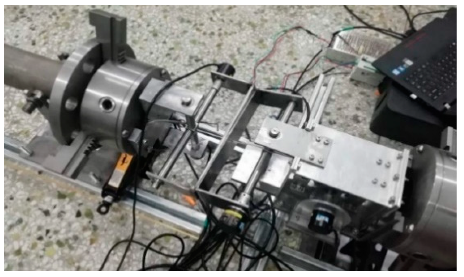
4.1. Composition of the Measuring Device
The pipeline measuring experimental device based on the flange center positioning is composed of the measuring device I, the measuring device II, the winch, the pipeline, the PLC (Programmable Logic Controller) and the upper computer, as shown in Figure 9.
Pipe I and pipe II are placed on the rails to move the pipe position. Pipe II can realize the horizontal and vertical swing adjustment and the vertical direction lift adjustment. During the experiment, different relative positional attitudes between the pipes can be simulated by moving pipe II and adjusting its horizontal, pitching, and vertical heights.
4.2. Testing Method and Recording Data
(1) First, the distance between the draw-out points of the two measuring devices from the end face of the pipe is measured. Then, adjust the height of pipe I to be equal to pipe II, and align the two rails of the installation pipe. Next, pipe II is moved to align the angle measuring mechanisms in the measuring device I and the measuring device II as shown in the Figure 10. At this time, the initial data of each sensor is collected by controlling the upper computer.
(2) Move pipe II to a different position on the rail. The measurement data of each sensor is observed and recorded on the host computer, and the relative distance and angle of the two pipes are measured by the laser range finder and the angle measuring instrument as reference values.
(3) The measurement experiment based on the flange center positioning uses a laser rangefinder to adjust the distance between the two pipeline centers to 2 m, 3 m, 4 m, 5 m, 6 m, and 7 m, and the angle measuring instrument is used to adjust the angles parameters ξx2, ξy2, and ξz2 formed by the axis of pipe II and the X, Y, and Z axes of the absolute coordinate system ΩR. It corresponds to the actual value in Table 2. Then the host computer calculates the projection values ORObx, OROby, ORObz, ξx2, ξy2, and ξz2. It corresponds to the measurements in Table 2.
4.3. Analysis of Measurement Data
Comparing Table 1 and Table 2, it is found that the experimental error of the measuring device based on the flange center positioning is smaller than that based on the outer circle positioning of the pipe, and the table shows the positioning method based on the flange center when the center distance between the two pipes is greater than 5 m and can reduce the error value of the measuring device by about 30%. In the 10 m working range, the error of Ox, Oy, and Oz was up to 56.49 mm, the precision was controlled within ±60 mm, and the system length measurement accuracy met the technical requirements. The maximum error of ξx, ξy and ξz was 0.588°, the accuracy was controlled within ±1°, and the system angle measurement accuracy met the technical requirements.
5. Conclusions
We have proposed a measuring device for measuring the pose of deep-sea pipelines. This measuring device measures the parameters used to calculate the pose of the pipeline using a drawstring pair. Moreover, we proposed a mathematical model of this device and solution formulas for calculating the pose of the pipeline. The measuring device we propose uses flanges for positioning on the pipe, which are smaller than the pin positioning error in the measuring device based on the outer circumference of the pipe. This measurement method is simpler than the measurement devices for underwater acoustic positioning and GPS positioning, and it is not easily interfered by the surrounding environment. At the same time, the structure and mathematical model of the proposed measuring device are simpler than those of the old tensioning rope measuring device.
In summary, the measurement device based on the flange center positioning has higher measurement accuracy, but the measurement device can be further improved. It can coincide the pull-out point of the measuring device based on the flange center positioning with the center point of the end face of the pipe. For example, the entire measuring device is transferred to the inside of the oil pipeline, and the mathematical model and solving formula of the measuring device will be simpler and more accurate. At this time, only the length of the drawstring and the data of the sensor need to be measured, and the spatial relative positions of the two pipes can be measured without knowing the two measurement parameters of ea and eb. Therefore, the error of the measuring device will be further reduced.
Author Contributions
The first author, Z.W., conceived the framework of the article and wrote the article; the second author, H.-x.D., analyzed the position and attitude measurement device based on the positioning of the outer wall of the submarine pipeline; the third author, T.W., designed and analyzed the measuring device based on the center positioning of submarine pipeline; the fourth author, B.Z., analyzes the experimental data of the measurement device based on the center positioning of the submarine pipeline. All authors have read and agreed to the published version of the manuscript.
Funding
This paper was funded by NSFC (Contract name: Research on ultimate bearing capacity and parametric design for the grouted clamps strengthening the partially damaged structure of jacket pipes). (Grant number: 51879063) and (Contract name: Research on analysis and experiments of gripping and bearing mechanism for large-scale holding and lifting tools on ocean foundation piles), (Grant number: 51479043).
Conflicts of Interest
The authors declare no conflict of interest.
References
- Yu, X.C.; Wang, C.S.; Li, B.; Cheng, B.; Li, Y.; Wang, Q. Pigging Solutions Study of Subsea Tieback Flow line for Deep-water Oil and Gas Fields in the South China Sea. Ocean Eng. Equip. Technol. 2017, 4, 199–205. [Google Scholar]
- Gao, Y.B.; Li, H.Q.; Chai, Y.P.; Ma, C.L. The Development of Deep Ocean High Technology. Ocean Technol. 2010, 29, 119–125. [Google Scholar]
- De Lucena, R.R.; Baioco, J.S.; De Lima, B.S.L.P.; Albrecht, C.H.; Jacob, B.P. Optimal design of submarine pipeline routes by genetic algorithm with different constraint handling techniques. Adv. Eng. Softw. 2014, 76, 110–118. [Google Scholar] [CrossRef]
- Laye, A.; Victoire, K.; Cocault-Duverger, V. Model-Centric Digital Subsea Pipeline Design Process and Framework. In Proceedings of the Offshore Technology Conference, Houston, TX, USA, 30 April–3 May 2018. [Google Scholar]
- Wang, L.Q.; Pan, Z.J.; Zhao, D.Y.; He, N.; Zhang, L. Technology of Pipeline Alignment in Subsea. Mach. Tool Hydraul. 2010, 38, 16–27. [Google Scholar]
- Wang, D.Y.; Zhu, A.D. Current Situation of Offshore Petroleum Equipment and Development Orientation of Localization. Chin. Pet. Mach. 2014, 42, 33–39. [Google Scholar]
- Liu, F. Method Study for Subsea Pipeline Spool Installation and Design in Special Working Condition. Pipeline Technol. Equip. 2018, 151, 34–41. [Google Scholar]
- Zhao, J.H.; Ouyang, Y.Z.; Wang, A.X. Status and Development Tendency for Seafloor Terrain Measurement Technology. Acta Geod. Cartogr. Sin. 2017, 46, 1786–1792. [Google Scholar]
- Dariusz, P.; Tomasz, T.; Michał, L. Using the geodetic and hydroacoustic measurements to investigate the bathymetric and morphometric parameters of Lake Hańcza. Open Geosci. 2015, 7, 1–8. [Google Scholar]
- Getmanov, V.G.; Modyaev, A.D.; Firsov, A.A. A method of measurement of the coordinates of a moving object with the use of a passive hydroacoustic detection and ranging system. Meas. Technol. 2012, 55, 248–256. [Google Scholar] [CrossRef]
- Tomasz, P. Correction of Navigational Information Supplied to Biomimetic Autonomous Underwater Vehicle. Pol. Marit. Res. 2018, 25, 13–22. [Google Scholar]
- Gamroth, E.; Kennedy, J.; Bradley, C. Design and testing of an acoustic ranging technique applicable for an underwater positioning system. Underwater Technol. 2011, 29, 4467–4477. [Google Scholar] [CrossRef]
- Wang, L.Q.; Wang, W.M.; Zhao, D.Y.; Cao, W.; Wang, C.D. A research into the Flange Connection Tooling for deep-sea pipelines. Nat. Gas Ind. 2009, 29, 89–97. [Google Scholar]
- Zhu, S.H.; Wei, X.C.; Liu, B. Study and application of measure technology by flange measure instrument to spool piece connection of subsea pipelines. Chin. Offshore Oil Gas 2008, 20, 342–349. [Google Scholar]
- Den, N.S.; Oljeselskap, A.S. System for subsea diverless metrology and hard-pipe connection of pipelines. U.S. Patent 6700835, 2 March 2004. [Google Scholar]
- Wang, W.M.; Wang, C.D.; Wang, L.Q. A novel deepwater structures pose measurement method and experimental study. Measurement 2012, 45, 1151–1159. [Google Scholar] [CrossRef]
- Shabani, M.; Gholami, A. Improved Underwater Integrated Navigation System using Unscented Filtering Approach. J. Navig. 2016, 69, 561–570. [Google Scholar] [CrossRef] [Green Version]
- Mallios, A.; Vidal, E.; Campos, R.; Carreras, M. Underwater caves sonar data set. Int. J. Rob. Res. 2017, 36, 1247–1256. [Google Scholar] [CrossRef]
- Han, W.H.; Zhou, J. Comparative Research of Corrosion Models for Corroded Submarine Pipelines. Pet. Eng. Constr. 2014, 40, 9–17. [Google Scholar]
Figure 1.
Measuring device based on the outer circle positioning of the pipeline.
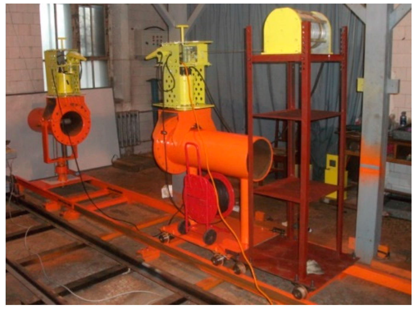
Figure 2.
Mathematical model I of the measuring device based on the outer circle positioning of the pipeline.
Figure 2.
Mathematical model I of the measuring device based on the outer circle positioning of the pipeline.

Figure 3.
Initialization of the measuring device.

Figure 4.
Schematic diagram of the measurement system based on flange center positioning.
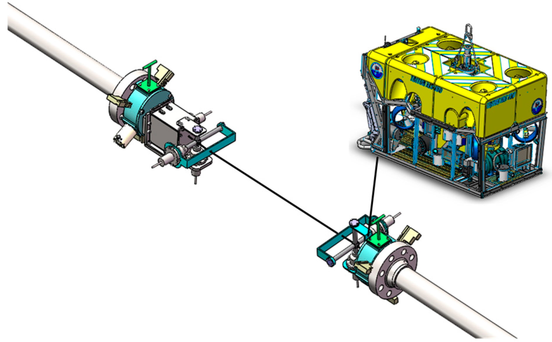
Figure 5.
Mathematical model II of the measuring device based on flange center positioning.
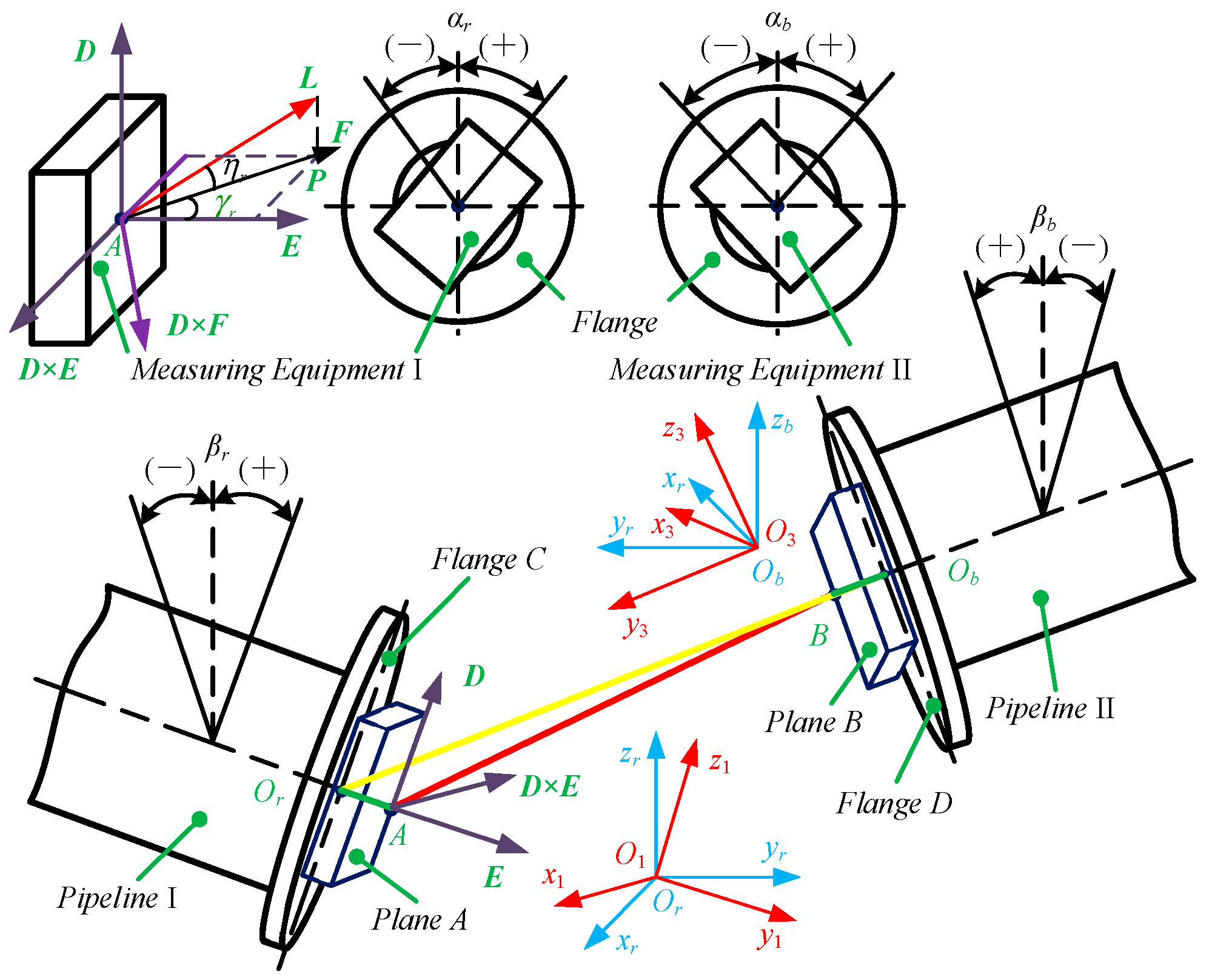
Figure 6.
Schematic diagram of angle parameters.
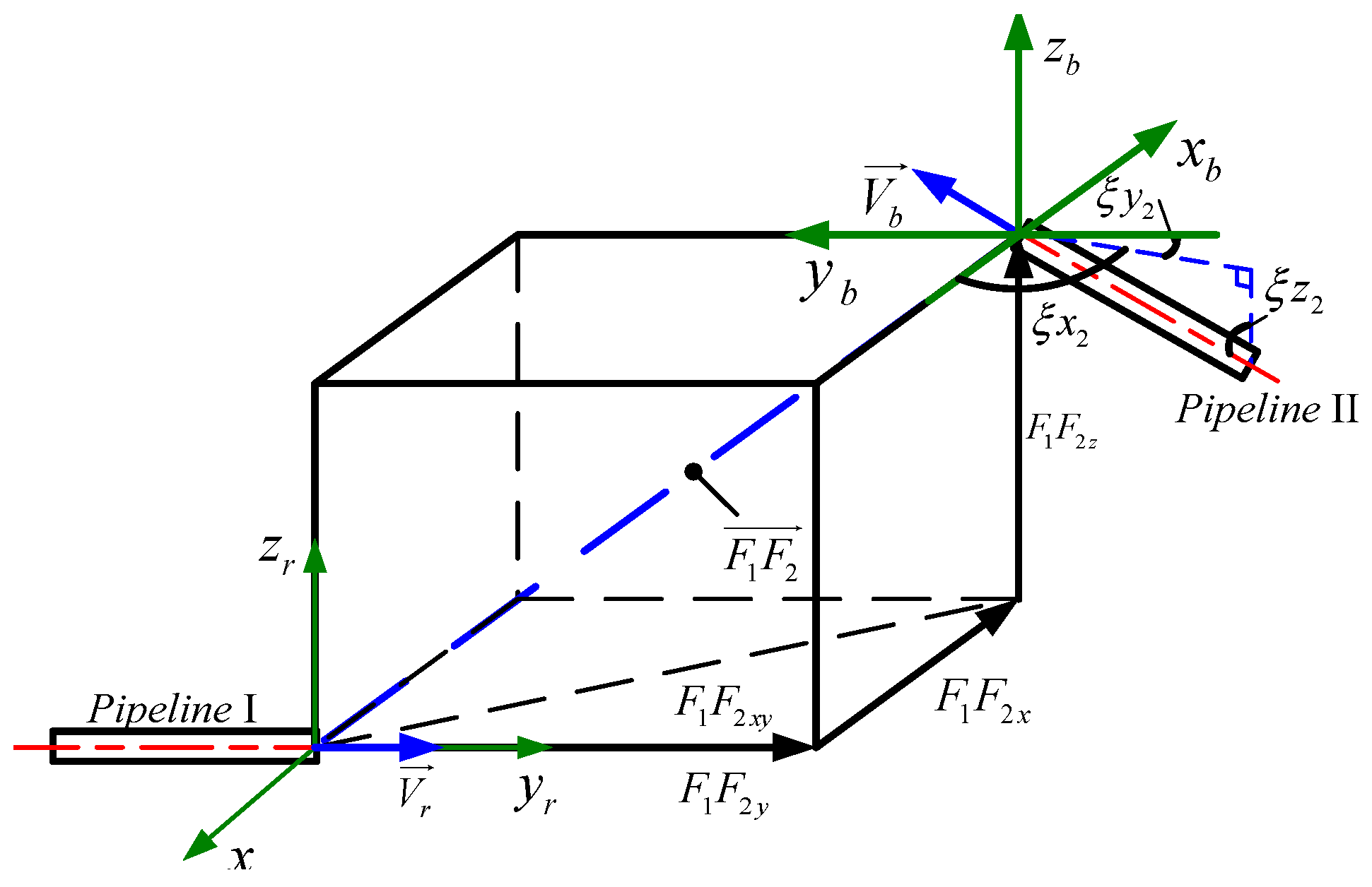
Figure 7.
Change surface map of C1. (a) corresponds to the same positive and negative αr and γr, (b) corresponds to the difference between αr and γr.
Figure 7.
Change surface map of C1. (a) corresponds to the same positive and negative αr and γr, (b) corresponds to the difference between αr and γr.
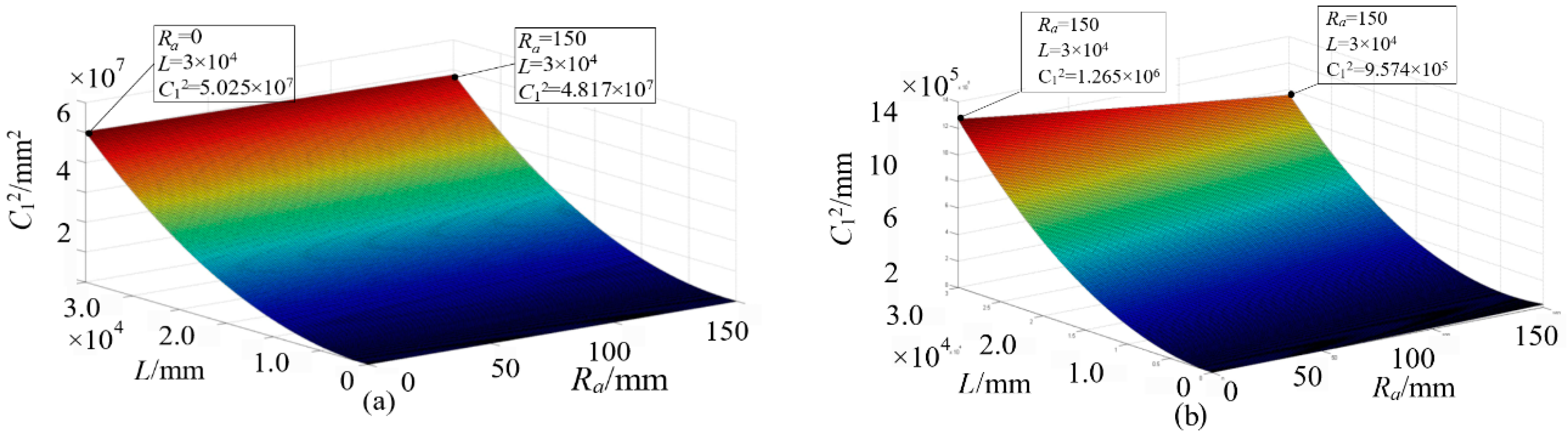
Figure 8.
Change surface map of C3. (a) corresponds to βb less than 0, (b) corresponds to βb greater than 0.
Figure 8.
Change surface map of C3. (a) corresponds to βb less than 0, (b) corresponds to βb greater than 0.
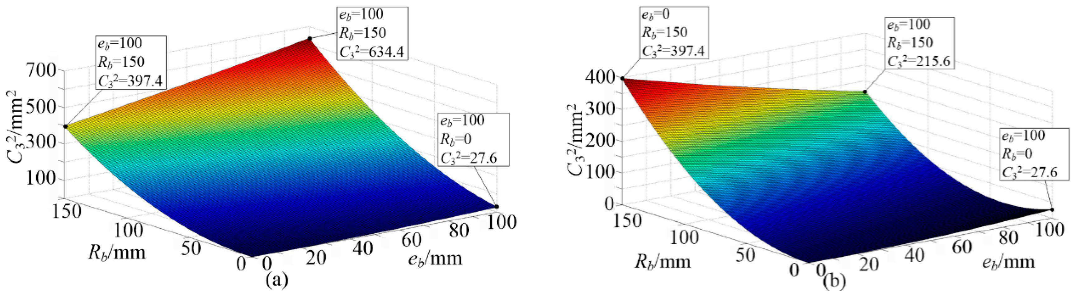
Figure 9.
Measuring device based on flange center positioning.
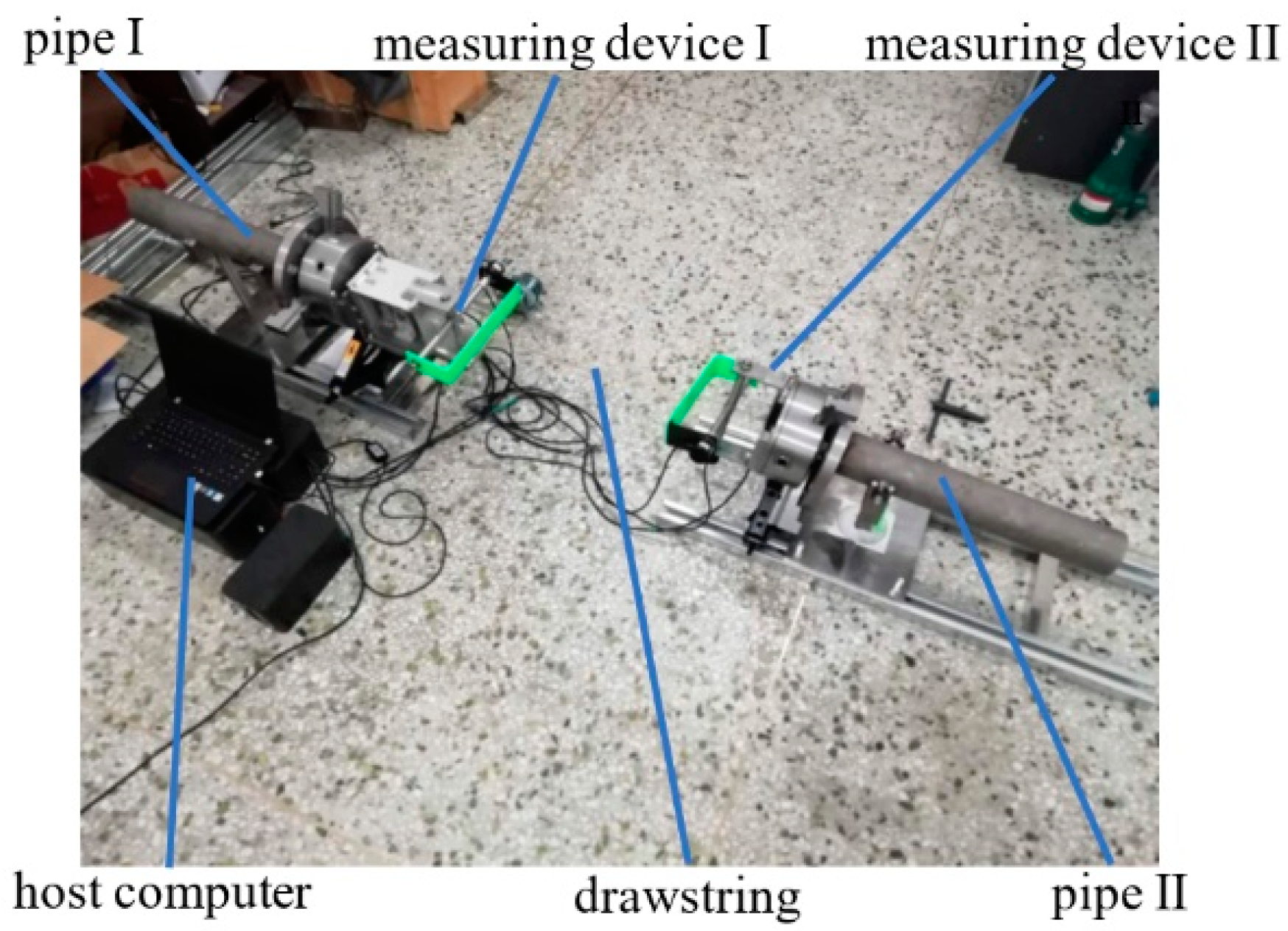
Figure 10.
Initialization of measuring device based on flange center positioning.


Table 1.
Experimental data of a measuring device based on the outer circle positioning of the pipe.
| Component of Measurements | Classification | 2 m | 3 m | 4 m | 5 m | 6 m | 7 m |
|---|---|---|---|---|---|---|---|
| actual value (mm) | 0.0 | 0.0 | 0.0 | 0.0 | 0.0 | 0.0 | |
| measurements (mm) | 5.4 | 11.2 | 25.4 | 21.3 | 38.3 | 40.4 | |
| actual value (mm) | 2000.0 | 3000.0 | 4000.0 | 5000.0 | 6000.0 | 7000.0 | |
| measurements (mm) | 1981.5 | 3009.9 | 4012.4 | 5022.5 | 6025.7 | 7032.6 | |
| actual value (mm) | 0.0 | 0.0 | 0.0 | 0.0 | 0.0 | 0.0 | |
| measurements (mm) | −6.6 | 12.2 | 12.8 | 27.7 | 54.5 | 68.8 | |
| actual value (mm) | 0.0 | 0.0 | 0.0 | 0.0 | 0.0 | 0.0 | |
| measurements (mm) | 0.2 | 0.5 | 0.8 | 1.1 | 1.2 | 1.1 | |
| actual value (mm) | 90.0 | 90.0 | 90.0 | 90.0 | 90.0 | 90.0 | |
| measurements (mm) | 89.8 | 89.5 | 89.2 | 88.9 | 88.8 | 88.9 | |
| actual value (mm) | 0.0 | 0.0 | 0.0 | 0.0 | 0.0 | 0.0 | |
| measurements (mm) | 0.3 | 0.2 | 0.8 | 0.5 | 0.7 | 1.2 |
Table 2.
Experimental data of measuring devices based on flange center positioning.
| Component of Measurements | Classification | 2 m | 3 m | 4 m | 5 m | 6 m | 7 m |
|---|---|---|---|---|---|---|---|
| actual value (mm) | 0.0 | 0.0 | 0.0 | 0.0 | 0.0 | 0.0 | |
| measurements (mm) | 4.7 | 9.2 | 13.1 | 16.8 | 23.1 | 30.5 | |
| actual value (mm) | 2000.0 | 3000.0 | 4000.0 | 5000.0 | 6000.0 | 7000.0 | |
| measurements (mm) | 1994.8 | 3004.1 | 4008.3 | 5014.8 | 6016.8 | 7025.2 | |
| actual value (mm) | 0.0 | 0.0 | 0.0 | 0.0 | 0.0 | 0.0 | |
| measurements (mm) | −2.1 | 9.6 | 11.9 | 18.8 | 32.5 | 46.9 | |
| actual value (mm) | 0.0 | 0.0 | 0.0 | 0.0 | 0.0 | 0.0 | |
| measurements (mm) | 0.2 | 0.3 | 0.6 | 0.9 | 1.0 | 1.1 | |
| actual value (mm) | 90.0 | 90.0 | 90.0 | 90.0 | 90.0 | 90.0 | |
| measurements (mm) | 89.8 | 89.5 | 89.3 | 89.0 | 89.1 | 88.9 | |
| actual value (mm) | 0.0 | 0.0 | 0.0 | 0.0 | 0.0 | 0.0 | |
| measurements (mm) | 0.2 | 0.3 | 0.7 | 0.6 | 0.8 | 0.9 |
© 2020 by the authors. Licensee MDPI, Basel, Switzerland. This article is an open access article distributed under the terms and conditions of the Creative Commons Attribution (CC BY) license (http://creativecommons.org/licenses/by/4.0/).
Share and Cite
MDPI and ACS Style
Wang, Z.; Dang, H.-x.; Wang, T.; Zhang, B. Development of a Position Measuring Device of a Deep-Sea Pipeline Based on Flange Center Positioning. J. Mar. Sci. Eng. 2020, 8, 86. https://doi.org/10.3390/jmse8020086
AMA Style
Wang Z, Dang H-x, Wang T, Zhang B. Development of a Position Measuring Device of a Deep-Sea Pipeline Based on Flange Center Positioning. Journal of Marine Science and Engineering. 2020; 8(2):86. https://doi.org/10.3390/jmse8020086
Chicago/Turabian StyleWang, Zhuo, Hong-xing Dang, Tao Wang, and Bo Zhang. 2020. "Development of a Position Measuring Device of a Deep-Sea Pipeline Based on Flange Center Positioning" Journal of Marine Science and Engineering 8, no. 2: 86. https://doi.org/10.3390/jmse8020086
Note that from the first issue of 2016, this journal uses article numbers instead of page numbers. See further details here.