Modelling the Wave Overtopping Flow over the Crest and the Landward Slope of Grass-Covered Flood Defences

Abstract

The wave overtopping flow can exert high hydraulic loads on the grass cover of dikes leading to failure of the cover layer on the crest and the landward slope. Hydraulic variables such as the near bed velocity, pressure, shear stress and normal stress are important to describe the forces that may lead to cover erosion. This paper presents a numerical model in the open source software OpenFOAM^® to simulate the overtopping flow on the grass-covered crest and slope of individual overtopping waves for a range of landward slope angles. The model provides insights on how the hydraulic forces change along the profile and how irregularities in the profile affect these forces. The effect of irregularities in the grass cover on the overtopping flow are captured in the Nikuradse roughness height calibrated in this study. The model was validated with two datasets of overtopping tests on existing grass-covered dikes in the Netherlands. The model results show good agreement with measurements of the flow velocity in the top layer of the wave, as well as the near bed velocity. The model application shows that the pressure, shear stress and normal stress are maximal at the wave front. High pressures occur at geometrical transitions such as the start and end of the dike crest and at the inner toe. The shear stress is maximal on the lower slope, and the normal stress is maximal halfway of the slope, making these locations vulnerable to cover failure due to high loads. The exact location of the maximum forces depends on the overtopping volume. Furthermore, the model shows that the maximum pressure and maximum normal stress are largely affected by the steepness of the landward slope, but the slope steepness only has a small effect on the maximum flow velocity and maximum shear stress compared to the overtopping volume. This new numerical model is a useful tool to determine the hydraulic forces along the profile to find vulnerable points for cover failure and improve the design of grass-covered flood defences.

1. Introduction

One of the main failure mechanisms of flood defences is wave overtopping [1]. Accurate descriptions of the overtopping flow are necessary for the assessment of flood defences. Overtopping waves exert high loads on the covers of flood defences while they run up the waterside slope, flow over the crest and down the landward slope. Earthen flood defences with a cover consisting of a top layer of sand or clay with vegetation are especially vulnerable to overtopping. The high flow velocities on the crest and landward slope can lead to significant erosion of the earthen cover. Long-term exposure of the dike cover to wave overtopping will finally lead to a breach.

A typical dike consists of a core, often a mixture of sand and clay, and a cover consisting of clay or sand with grass vegetation on top (Figure 1a). Grass can significantly increase the erosion resistance of both clay and sand covers [2], but affects the hydraulic load of the overtopping wave as well. Grass covers increase the roughness of the dike cover compared to bare clay covers, which can slow down the overtopping wave and reduce the hydraulic load.

Erosion of the cover layer occurs when the hydraulic load exceeds the strength of the cover. High hydraulic loads leading to cover failure are related to three processes: (1) high flow velocities at the wave front, (2) wave impact at geometric changes and (3) turbulence leading to high stresses on the cover. These high loads result in large hydraulic forces pulling both horizontally and vertically on the cover leading to erosion once the cover strength is exceeded. Wave overtopping tests on grass-covered dikes have shown a large variability in the locations of cover erosion and failure [4]. Knowledge of the location of erosion is still missing because it is unknown how these loads change along the profile and how the load is affected by cover type, transitions or irregularities, such as holes and bumps [5,6].

The hydraulic forces on the grass cover across the dike crest and landward slope are unknown because existing methods are not able to compute the hydraulic forces along the dike profile. The hydraulic load in most erosion models for earthen flood defences is solely described by the maximum flow velocity $U_{max}$ (Figure 1b) anywhere along the slope, for example the cumulative overload method [7] and the erosion model of Hoffmans [2]. Several formulas for the maximum flow velocity are developed based on experimental data [7,8,9,10] and theory [11,12]. These formulas described the flow in an idealised manner, and they can often only be applied to uniform crests or slopes. Variation in slope angle or cover type can be modelled using the formulas of Van Bergeijk et al. [12]; However, smaller irregularities along the profile, such as existing erosion holes or bumps, cannot be described by these idealised models. Moreover, descriptions of the maximum flow velocity do not include any information on the vertical flow structure. The formulas for the maximum flow velocity are all validated with measurements in the top layer of the overtopping flow where the velocity is highest. However, the hydraulic load on the cover is determined by the flow velocity and turbulence close to the bed. Thus, models are required that do not solely describe the flow in the top layer, but also the flow near the bed.

Multiple studies have indicated that horizontally and vertically varying hydraulic variables such as the pressure, normal stress, shear stress and shear velocities are important to understand failure by cover erosion or instability [9,13,14,15]. The pressure and normal stresses are required to compute the forces due to wave impact [15]. Zhang et al. [14] identified cover erosion caused by a combination of normal and shear stress as the main mechanism of dike failure. The pressure on vertical walls by overtopping waves has been measured in experiments [13,14]. However, it is difficult to measure the pressure and stresses on the dike cover during flume and field tests. Thus, the distribution of the near bed velocity, pressure and stresses along a dike profile are unknown.

Computational fluid dynamics (CFD) models can resolve these hydraulic variables and are an efficient tool to obtain insights into the wave overtopping flow. Recent numerical models for wave overtopping are focused on the waterside of flood defences to determine the structural response of breakwaters [16,17,18], the wave impact on vertical walls [19,20] or the amount of wave overtopping [21,22]. These numerical models solve different equations and methods to simulate the flow: the momentum equations using the smoothed particle hydrodynamics method [17,19], the non-linear shallow water equations in 2D without a turbulence model [21,22] and the Reynolds-averaged Navier–Stokes (RANS) equations using the volume of fluid method in 2D [18,20,21] or 3D [16]. These models are not yet applied to flood defences with an earthen cover, but only to hard structures with revetments. Bomers et al. [6] developed the first numerical model for overtopping flow over a grass-covered dike. The model uses commercial software to solve the 2D RANS equations with the finite element method. The domain includes only a small part of the upper slope and the wave overtopping simulator, which means that the model is not generally applicable. The flow acceleration down the landward slope is not simulated in these studies, because the mentioned numerical models do not include the landward slope of the flood defence or—in case of breakwaters—the landward slope is located mostly below the still water level. Additionally, the variables essential to determine failure of the grass cover such as the shear and normal stress have not been modelled previously, which means that the locations where these variables are maximal remain unknown.

The objective of this study is to develop a numerical model in the open source software OpenFOAM^® to simulate the flow of an individual overtopping wave over the crest and the landward slope of a grass-covered flood defence. The numerical model covers a variety of output variables including the flow velocity, layer thickness, pressure, shear stress and normal stress. This numerical study provides insights on the dominant hydrodynamic forces working on the grass cover of dikes and how these forces change along the dike profile. Moreover, the hydraulic forces are computed at every location on the dike crest and landward slope to identify locations where the hydraulic loads are high and therefore vulnerable to failure by wave overtopping. Two datasets of overtopping experiments on grass-covered dikes in the Netherlands are used to calibrate and validate the model. These datasets together with the model input variables are described in Section 2. Section 3 describes the model settings and the output variables. The model is validated for the layer thickness, the flow velocity and pressure on the crest and landward slope (Section 4). Additionally, the vertical flow structure is validated with measurements of the flow velocity near the bed and in the top layer of the flow. The pressure, shear stress and normal stress on the cover are presented to show how the hydraulic load changes along the profile for the overtopping wave. Next, the model is applied to a grass-covered dike with varying slope steepness to show how the hydraulic loads are affected by the geometry (Section 4.4). Finally, the results are discussed in Section 5 followed by the conclusions in Section 6.

2. Measured Overtopping Variables

2.1. Data of the Field Tests

Overtopping tests on grass-covered dikes in the Netherlands were performed with the Wave Overtopping Simulator (WOS) [23]. Flow velocity and layer thickness as a function of time were measured during two field tests: Vechtdijk [24] and Millingen a/d Rijn [25]. Additionally, the pressure as a function of time was measured at Millingen a/d Rijn. The hydraulic variables were measured for individual overtopping waves resulting in 24 waves for Vechtdijk and 28 waves for Millingen a/d Rijn. The grass cover did not erode during these hydraulic tests.

2.1.1. Vechtdijk

The profile at Vechtdijk has an average slope steepness of 1:5 and a slope length of approximately 15 m [24] (Figure 2a). The layer thickness h as a function of time t was measured with surfboards at five locations V1–V5 [26] (Figure 1). A paddle wheel was mounted to the surfboard at locations V3 and V5 to measure the flow velocity in the upper layer $u_t$ as a function of time (

Table 1. Overview of the measurements with the measurement locations of the layer thickness h, the flow velocity in the top layer $u_t$ and the flow velocity near the bed $u_b$ together with the released overtopping volumes during the tests with the wave overtopping simulator (Figure 2). The volumes were released more than once resulting in the total number of waves.

Experiment	$\mathit{h}\left(\mathit{t}\right)$	${\mathit{u}}_{\mathit{t}}\left(\mathit{t}\right)$	${\mathit{u}}_{\mathit{b}}\left(\mathit{t}\right)$	Volumes (m${}^3$/m)	Waves
Vechtdijk	V1, V2, V3, V4, V5	V3, V5	V3	0.2, 0.4, 0.6, 0.8, 1.0, 2.0, 3.0, 4.0	24
Millingen	M1, M2, M4, M6, M8	M1, M2, M4, M6, M8	M3, M5, M7	0.4, 0.6, 0.8, 1.0, 1.5, 2.0, 2.5, 3.0, 4.0, 5.0, 5.5	28

). Another paddle wheel was placed in the ground at V3 to measure the flow velocity $u_b$ near the bed. The five locations were 3, 5, 7, 11 and 15 m away from the outlet of the WOS. Individual overtopping waves with volumes between 0.2 m${}^3$/m and 4 m${}^3$/m were released (Table 1). Eight different volumes were tested, and each volume was measured three times resulting in a total of 24 overtopping waves.

A much smaller layer thickness was measured at V4 compared to the measurements at the other locations for the overtopping volumes of 0.2–1 m${}^3$/m. These outliers were removed by the study of SBW (Sterkte en Belastingen Waterkeren) [26] resulting in no available data for the layer thickness at V4 for these volumes. Additionally, the flow velocity in the top layer $u_t$ at location V3 was not available for the overtopping volumes of 2–4 m${}^3$/m, because the paddle wheel was dismounted during these measurements. Only measurements at location V1 were available for the overtopping volume of 0.2 m${}^3$/m because the layer thickness at the other locations was too small to be measured.

2.1.2. Millingen a/d Rijn

The profile at Millingen a/d Rijn gradually changes from a steep upper slope of 1:3 to a gentler lower slope of 1:6 (Figure 2b). The layer thickness and flow velocity were measured at eight locations M1–M8 [25]. The first measurement location M1 was located 2 m from the outlet of the WOS. The other measurement locations were located at a cross-dike distance x = 2.00, 2.95, 3.95, 4.85, 5.80, 6.75 and 15.30 m. Eleven different volumes were released varying from 0.4 m${}^3$/m to 5.5 m${}^3$/m with a total of 28 individual overtopping waves (Table 1). The volumes of 0.4 m${}^3$/m to 2.5 m${}^3$/m were tested twice. Measurements of the larger volumes (3.0–5.5 m${}^3$/m) were repeated resulting in three or four measurements per volume. The layer thickness as a function of time was measured at five locations (Table 1). The flow velocity was measured at all eight locations with a paddle wheel. At M1, M2, M4, M6 and M8, the paddle wheel was mounted on the surfboard to measure the flow velocity in the top layer $u_t$. At the other three locations, the paddle was mounted on a plate to measure the flow velocity near the bed $u_b$. The measurement instruments at locations M3, M5, M7 and M8 did not work properly during the repeated measurements series of the volumes 3.0–5.0 m${}^3$/m leading to extremely low flow velocities ($\le$0.5 m/s) [25]; thus, these measurements are excluded in this study.

Additionally, the pressure was measured for the same overtopping volumes with pressure sensors located at $x=11.00$ m and $x=15.65$ m (Figure 2b). The pressure was measured both near the dike surface and around 10 cm below the surface with a frequency of 5000 Hz.

2.2. Model Input Variables

The overtopping waves at the crest were characterised by the flow velocity in the upper layer u (m/s) and the layer thickness h (m), which were used to build the boundary conditions for the model. These variables depended on the overtopping volume V (m${}^3$/m) and varied along the profile. Van der Meer et al. [7] derived empirical formulas for the maximum flow velocity $U_{max}$ (Equation (1)) and maximum layer thickness $h_{max}$ (Equation (2)) on a grass-covered dike crest.

$$U_{max}=5.00V^{0.34}$$

(1)

$$h_{max}=0.133V^{0.5}$$

(2)

The variation in the maximum flow velocity along the dike profile determines the most likely location of erosion and can be described by an acceleration factor [27] or analytical formulas [9,12].

Experiments [7,28] have shown that the flow velocity and layer thickness instantaneously increase to their maximum followed by a slower decrease to zero as the wavefront passes (Figure 1b). The time difference between the moment the wavefront arrives and the flow velocity or layer thickness becomes zero is called the overtopping period $T_0$ (s). Hughes [3] used an idealised saw-tooth shape to describe the layer thickness and flow velocity as a function of time t (Figure 1b).

$$\begin{array}{ccc}h(x,t)=h_{max}\left(x\right){\left[1-\frac{t}{T_0}\right]}^a& \hfill & \mathrm{for}0\le t\le T_0\hfill \end{array}$$

(3)

$$\begin{array}{ccc}u(x,t)=U_{max}\left(x\right){\left[1-\frac{t}{T_0}\right]}^b& \hfill & \mathrm{for}0\le t\le T_0\hfill \end{array}$$

(4)

where the maximum layer thickness $h_{max}$ and the maximum flow velocity $U_{max}$ at the wavefront depend on the cross-dike coordinate x. The factors a and b describe the shape of the decrease over time. According to Verhagen and Van der Meer [29] and Hughes [3], the shape of the flow velocity and layer thickness is triangular with $a=b=1$. The overtopping period depends on the overtopping volume and is calculated using the empirical formula of Van der Meer et al. [7] for the overtopping period on the crest.

$$T_0=4.4V^{0.3}$$

(5)

The three empirical formulas of Van der Meer et al. [7] were based on measurements of overtopping volumes in the range of 0.2–5.5 m${}^3$/m; thus, the modelled waves in this study were within the application range.

3. Model Setup

This paper presents a new numerical model to determine in detail the hydraulic load on the dike cover. The numerical model simulates the flow over the crest and the landward slope of one overtopping wave. The numerical value for the roughness of a grass-cover is unknown; thus, the roughness height is calibrated. Next, the model was validated for a wide range of overtopping volumes using the measurements of the field tests on grass-covered dikes. The maximum velocity, maximum layer thickness and maximum pressure were used for both model calibration and validation. Additionally, the modelled flow velocity in the top layer and near the bed was validated with measurements. In the end, the pressure, the normal stresses and the shear stresses along the dike profile were computed to analyse the variation in the hydraulic load along the profile. First, the load was computed along the profiles of Millingen a/d Rijn and Vechtdijk to identify locations with high loads. Next, the load was computed for a grass-covered dike with varying slope steepness to show the effect of geometry on the maximum load.

3.1. Model Specifications

The numerical model was developed in the open-source software OpenFOAM^®, which solves the two-phase Reynolds-averaged Navier–Stokes equations using the finite volume method,

$$\nabla \overline{u}=0$$

(6)

$$\frac{\partial \rho \overline{u}}{\partial t}+\rho (\overline{u}·\nabla )\overline{u}=\nabla (\mu \nabla ·\overline{u})-\nabla p+F$$

(7)

with the velocity vector $\overline{u}$, the density of the fluid $\rho$, the dynamic viscosity $\mu$, the pressure p and the forces F related to bottom friction, surface tension and gravity. The equations were solved with the PIMPLE algorithm, which is a combination of the SIMPLE (semi-implicit method for pressure-linked equations) and PISO (pressure implicit with splitting of operators) algorithms resulting in better stability of the model results [30].

The water-air interface was solved using the volume of fluid method, where the fluid properties $\xi$ in every cell are determined from the average of water and air properties using the water fraction $\alpha$:

$$\xi =\alpha {\xi }_{water}+(1-a){\xi }_{air}$$

(8)

where the water fraction $\alpha$ is 0 for air, 1 for water and between 0 and 1 for mixtures of air and water. The interIsoFoam solver of the IsoAdvector algorithm was selected to solve the water-air interface sharply and efficiently [31]. The IsoAdvector algorithm defines an isoface in every cell, which is an interface between water and air. The advection of these isofaces was computed to determine the amount of water and air flowing to the neighbouring cells on the interface. The MULESalgorithm—standard in OpenFOAM^® and used in other overtopping studies [18,20,32]—does not define these interfaces and is only applicable to flows with a Courant number $\le 0.1$, while the IsoAdvector algorithm is applicable to flows with a maximum Courant number of 1.

For solving the turbulence in the flow, the $k-\omega$ SST turbulence model—a combination of the $k-ϵ$ and $k-\omega$ model—was selected to simulate the turbulence in both the free-stream region and the boundary layer [33]. In these models, SST stands for shear stress transport, and the symbols correspond to the turbulent kinetic energy k, the rate of dissipation of turbulent kinetic energy $ϵ$ and the specific rate of dissipation $\omega$. The $k-\omega$ SST turbulence model uses the $k-ϵ$ turbulence model in the free-stream region and switches to the $k-\omega$ model near the wall to model the turbulence in the boundary layer.

The model domain covers the dike crest and the landward slope (Figure 2). The 2DVmesh was generated using the snappyHexMesh utility. For the Vechtdijk case, the horizontal grid size $\Delta x$ was 3 cm, and the vertical grid size $\Delta z$ was 2 cm. The grid sizes for the Millingen a/d Rijn case were larger with $\Delta x=5$ cm and $\Delta z=3$ cm, because the overtopping volumes and the length of the dike profile were larger (Figure 3). The bottom cells were parallel to the dike surface, and the vertical grid size was constant for the first 0.5 m above the dike surface and increased to 2$\Delta z$ for the next layer located from 0.5 m to 1.5 m above the dike surface. These settings resulted in a hexahedral mesh with 25,956 cells for the Millingen a/d Rijn case and 33,440 cells for the Vechtdijk. Tests with different grid sizes and shapes showed that these settings were optimal and the grid size did not affect the results (Section 5.4.3). Finer vertical grid seizes were not possible due to the bed roughness, while a courser grid size was not able to simulate the vertical velocity profile accurately.

The roughness of the grass-cover was included in the turbulence model using the roughness constant $C_s$ (-) and the Nikuradse roughness height $K_s$ (m) on the dike surface. The roughness constant $C_s$ represents the shape and spacing of the roughness elements, and the roughness height $K_s$ represents the height of the elements [34]. Nikuradse [34] empirically determined a value of 0.5 for the constant $C_s$, which is representative of uniform, closely packed sand grains. The values of both variables were unknown for grass covers under overtopping waves. In this model, the roughness constant $C_s$ was set to 0.5, and the roughness height $K_s$ was determined from calibration. It is important to notice that the roughness height $K_s$ should not be larger than half the cell size. Roughness elements larger than the grid size need to be resolved in the grid itself and cannot be modelled using the roughness height. For example, the bump at the toe of Millingen a/d Rijn around $x=$ 20–22 m (Figure 2b) was larger than the grid size and was resolved in the grid (Figure 3).

The computational time step was set to 0.001 s, but the time step was adjustable with a maximum Courant number of 1 and a maximum time step of 1 s. The writing time step was fixed at 0.1 s. Simulation of one individual wave over the crest and landward slope took between 5 and 20 min depending on the overtopping volume using a standard computer with an Intel core^TM i7-9700 GHz(x12) processor using only one core.

3.1.1. Boundary Conditions

New boundary conditions were implemented in OpenFOAM at the start of the model domain. These boundary conditions were based on the flow velocity in the top layer and the layer thickness as a function of time of the individual overtopping wave at the start of the domain. Firstly, the boundary conditions for the layer thickness were transferred to the boundary conditions for the water fraction $\alpha$ because the layer thickness was not a variable in the OpenFOAM software. The water fraction at the start of the domain was set to 1 (water) when the cell height $y_i$ was smaller or equal to the sum of the layer thickness and the dike height H, otherwise the water fraction was set to 0 (air).

$${\alpha }_i=\left\{\begin{array}{cc}1,\hfill & \mathrm{if}{y}_i\le h_j+H\hfill \\ 0,\hfill & \mathrm{if}{y}_i>h_j+H\hfill \end{array}\right.$$

(9)

with ${\alpha }_i$ the water fraction in the cell at height $y_i$ and $h_j$ the layer thickness at time step j. Next, various functions of the flow velocity as a function of height were studied as boundary conditions at the start of the domain, including a logarithmic wall function (Equation (14)). However, this resulted in a time lag between the model results and measurements since the turbulence model already accounted for the vertical flow structure (Section 4.2.2). For that reason, the flow velocity in every cell $u_i$ at the boundary containing water was set to the flow velocity in the top layer $u_{t,j}$ at time step j resulting in an accurate boundary condition with no time lag between the model results and the measurements.

$$u_i=\left\{\begin{array}{cc}{u}_{t,j},\hfill & \mathrm{if}{y}_i\le h_j+H\hfill \\ 0,\hfill & \mathrm{if}{y}_i>h_j+H\hfill \end{array}\right.$$

(10)

A no-slip boundary condition was set for the flow velocity on the dike surface. The upper boundary was open to the atmosphere to allow the air flowing in and out of the domain at locations of low and high pressure. The end of the model domain was set to an open outlet where water and air could flow out freely without influencing the flow in the model domain.

The flow velocity in the top layer and the layer thickness as a function of time of the individual overtopping wave were the required boundary conditions at the start of the domain. The model domain started halfway of the crest at the location of the first measurement point for the Millingen a/d Rijn case and at the end of the wave overtopping simulator for the Vechtdijk case. For simulations of Millingen a/d Rijn, the measured flow velocity and layer thickness at M1 were used as boundary conditions for the model. The measured layer thickness and flow velocity were transferred from the measured frequency of 125 Hz to 10 Hz using a time average to match the writing time step of the model.

The flow velocity at Vechtdijk was not measured on the crest; the first measurement location of the velocity was halfway of the slope. Using these measurements as boundary conditions would limit the model domain to the lower slope resulting in a small number of measurements for model validation. Therefore, we used the formulas of Van der Meer et al. [7] and Hughes [3] to generate the boundary conditions at the crest for the Vechtdijk case. First, the maximum flow velocity $U_{max}$, the maximum layer thickness $h_{max}$ and the overtopping period $T_0$ of each overtopping volume were calculated using Equations (1), (2) and (5), respectively. Next, the flow velocity $u(x=0,t)$ and layer thickness $h(x=0,t)$ were calculated using Equations (3) and (4) with the shape factors $a=b=1$. These generated time series of the flow velocity and layer thickness were used as boundary conditions for the Vechtdijk case.

3.1.2. Model Output Variables

The model output included the flow velocity and water fraction $\alpha$ for every cell at every writing time step. The layer thickness was determined from the model output of the water fraction $\alpha$. The layer thickness was defined as the highest cell for which $\alpha$ was larger than 0.6. This meant that in case the cell was filled with more than 60% of water, we assumed the cell was completely filled with water while the cell was empty when the cell contained less than 60% of water.

The flow velocity was measured using paddle wheels that were either mounted on the surfboard (V3, V5, M1, M2, M4, M6, M8) or on a plate on the ground (V3, M3, M5, M7). In the first case, the flow velocity in the upper part of the flow was measured. The modelled flow velocity at the height of the modelled layer thickness ($z=h$) was used for comparison with these measurements. In cases where the paddle wheel was mounted on a plate on the ground, the flow velocity in the first 2–3 cm water depth was measured. This velocity was compared to the modelled flow velocity in the centre of the second cell at a height of 3 cm for Vechtdijk and 4.5 cm for Millingen (Section 5.4.2).

The shear stresses on the dike cover were determined using the wallShearStress utility in OpenFOAM. The wall shear stress ${\tau }_w$ is computed as:

$${\tau }_w={\nu }_{eff}\frac{\partial U}{\partial y}$$

(11)

with the flow velocity parallel to the wall U, the distance to the wall y and the effective viscosity ${\nu }_{eff}$. The effective viscosity accounts for both laminar as turbulent contributions, where the turbulent contribution is affected by the wall roughness. The wallShearStress utility was modified to obtain the stresses normal and parallel to the dike surface using the normal vector of each boundary cell resulting in the normal stress ${\tau }_n$ and the shear stress ${\tau }_s$ on the cover (Figure 1a) for every boundary cell at every writing time step.

The pressure p on the dike surface was obtained from the model results using a sampling function that calculated the pressure on the dike surface instead of the cell centre. The sampled pressure was the sum of the hydrostatic pressure $p_s$ and the dynamic pressure, which was calculated in OpenFOAM using the flow velocity u and the density $\rho$ [30].

$$p=p_s+0.5\rho {|u|}^2$$

(12)

3.2. Calibration of the Roughness Height

The roughness height $K_s$ is unknown for grass covers and this type of flow in OpenFOAM^® and was therefore calibrated. The dataset of Millingen a/d Rijn included the widest range of overtopping volumes and the most measurement locations; thus, one overtopping wave per volume of Millingen a/d Rijn was used for calibration of the roughness height. The 11 volumes (Table 1) were modelled for 10 values of the roughness height in the range of 1–10 mm with steps of 1 mm. Smaller values of the roughness height did not lead to better results, and the maximum roughness height for calibration was set to 10 mm to stay within the application limit of the turbulence model (Section 3.1). The measured flow velocity and layer thickness at M1 were used as boundary condition, which left the flow velocity at the other seven locations (M2–M8) for calibration of the roughness height. The roughness height was calibrated on the maximum flow velocity using the dimensionless root-mean-squared error E (-) to compare the results of the various volumes:

$$E=\frac{\sqrt{{\sum }_{i=1}^N{\left(U_{max,m}\left\{i\right\}-U_{max,o}\left\{i\right\}\right)}^2/N}}{\overline{U_{max,o}}}$$

(13)

with the number of data points N, the maximum velocity of the model $U_{max,m}$, the maximum velocity of the observations $U_{max,0}$ and the average of the observed maximum velocity $\overline{U_{max,o}}$ per volume. The dimensionless root-mean-squared error E (-) was determined for the 11 overtopping waves using the maximum flow velocity at M2–M8 leading to $N=77$ points per roughness height. The optimal value of the roughness height was the height with the smallest dimensionless root-mean-squared error E. An error of 0.1 meant that the difference between the modelled and measured flow velocity was 10% of the averaged measured flow velocity. We assumed that the roughness height was uniform along the dike profile and representative for grass covers in the Netherlands following the approach of Van Hoven et al. [25] and Aguilar-López et al. [5]. Thus, the calibrated value was assumed to be applicable for both the Vechtdijk and the Millingen a/d Rijn cases.

3.3. Model Validation

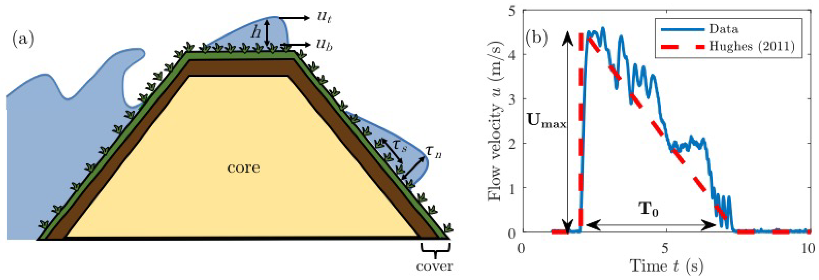
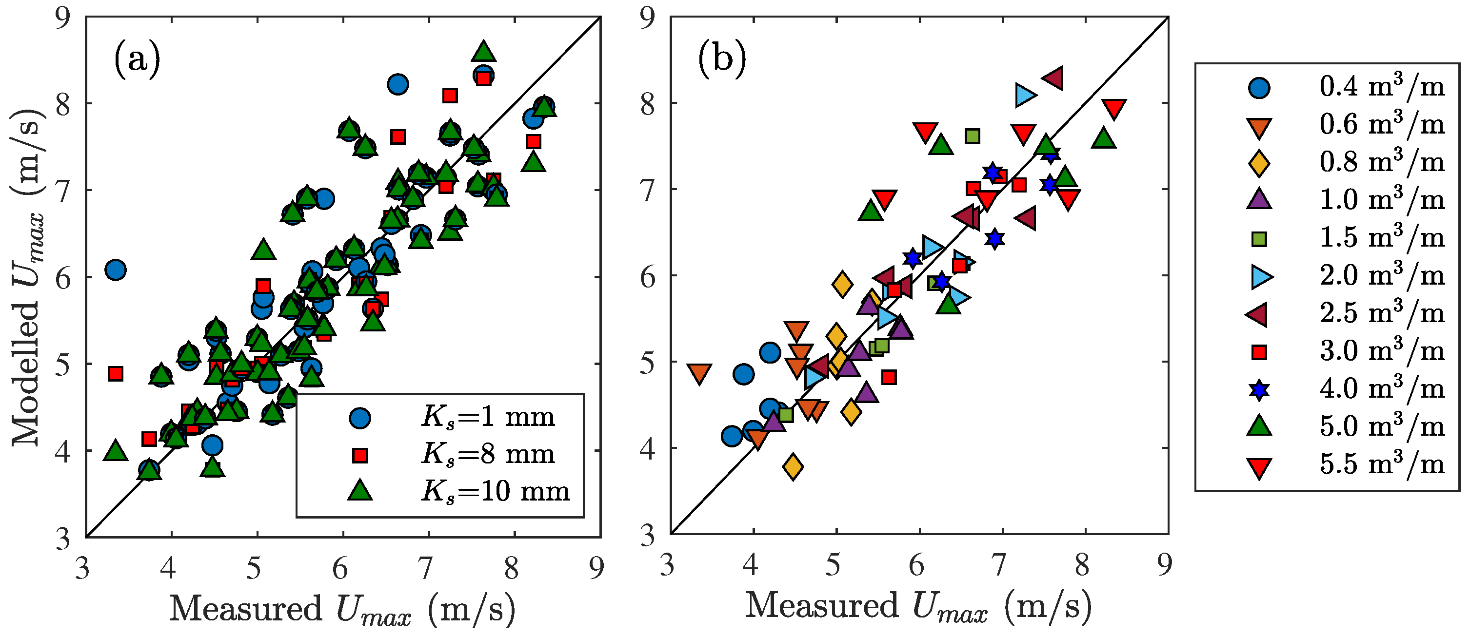
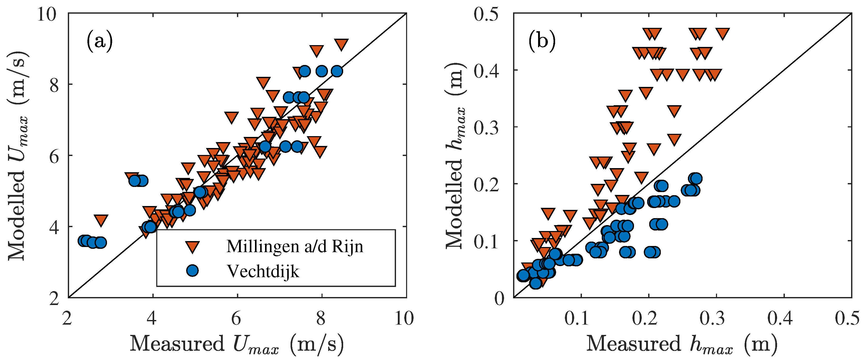
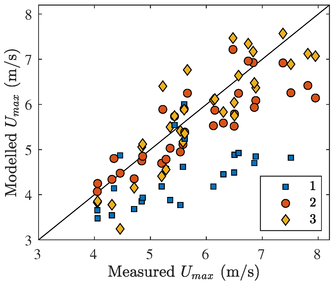
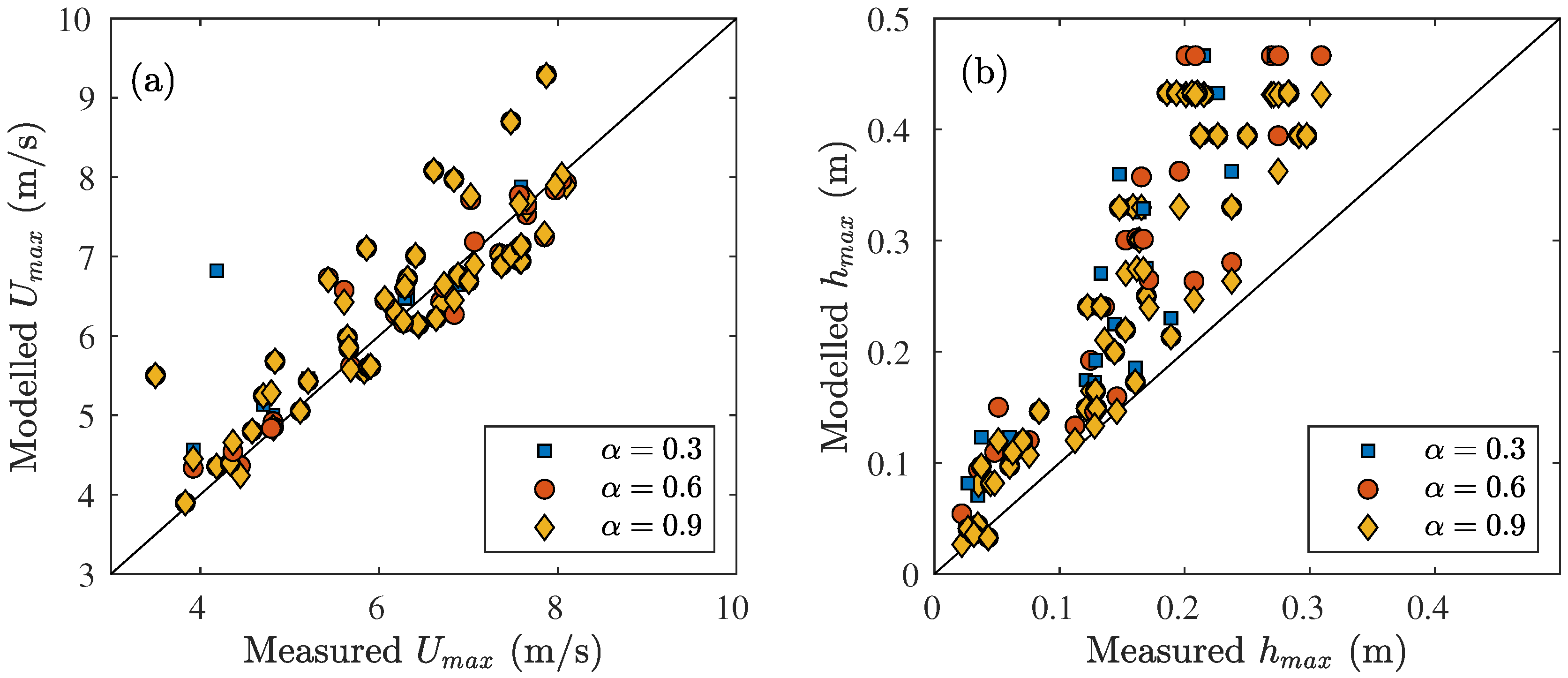
3.3.1. Maximum Flow Velocity and Layer Thickness

The remaining 17 overtopping waves of the Millingen a/d Rijn dataset together with the Vechtdijk dataset were used to validate the model. The measurements at location M1 of the 17 remaining overtopping volumes were used as boundary conditions for Millingen a/d Rijn. Although the waves had approximately the same volume, every released wave was unique. Thus, every released wave volume could be seen as a separate volume resulting in 17 independent simulations for validation. The maximum measured velocity was reported at all seven measurement locations M2–M8 for the first 11 overtopping volumes, but for the repeated measurements series of the volumes 3.0–5.0 m${}^3$/m, only the data of measurement locations M2, M4 and M6 were available (Section 2). This led to $N=11\times 7+6\times 3=95$ values for model validation for the flow velocity. The layer thickness was measured at four locations (M2, M4, M6 and M8) for the first 11 overtopping volumes and at three locations (M2, M4 and M6) for the other seven volumes. A measured layer thickness smaller than 60% of the cell height was removed, because in these cases, the modelled layer thickness was zero. For the Millingen a/d Rijn case, only one measurement was smaller than 1.8 cm resulting in $N=11\times 4+6\times 3-1=61$ values for model validation of the layer thickness. Validation of the Millingen a/d Rijn case showed how accurate the model could predict the propagation of the overtopping wave along the dike profile, while the validation of the Vechtdijk showed the accuracy of the model simulations for wave conditions based on the empirical equations for the overtopping variables on the crest.

The boundary conditions for the Vechtdijk were generated using the overtopping volume (Equations (1), (2) and (5)). In this case, the boundary conditions for overtopping waves with the same volume were equal, and the waves could not be seen as separate events leading to only eight model simulations (Table 1). The maximum velocity in the top layer at locations V3 and V5 was used to validate the model. Since the flow velocity at V3 was not reported for the three volumes of 2 m${}^3$/m, 3 m${}^3$/m and 4 m${}^3$/m, there were $N=5\times 3\times 2+3\times 3\times 1=39$ values of the maximum velocity for model validation. The layer thickness was measured at four locations (V1, V2, V3, V5) for the volumes 0.2–1.0 m${}^3$/m and at all five location for volumes 2–4 m${}^3$/m. Again, the measured layer thickness smaller than 60% of the grid size was removed, which were 17 measurements in the Vechtdijk case for the small overtopping volumes. Finally, we were left with $N=5\times 3\times 4+3\times 3\times 5-17=88$ points for model validation of the layer thickness for the Vechtdijk case.

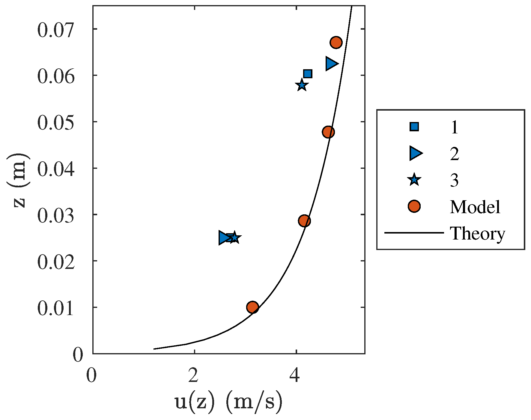
3.3.2. Vertical Flow Structure

The flow velocity was measured both near the bed at 2–3 cm height and in the top of the overtopping wave at location V3 of Vechtdijk. Thus, it was possible to validate the vertical flow structure of the model at this location. The modelled flow velocity at every wetted cell was compared to the measured layer thickness at $z=2.5$ cm and $z=h$. Moreover, the modelled vertical structure was compared to the theoretical logarithmic law of the wall [35],

$$u\left(z\right)=\frac{u_{\tau }}{\kappa }ln\left(\frac{z}{z_0}\right)$$

(14)

with the friction velocity $u_{\tau }$ and the von Kármán constant $\kappa =0.41$. The height from the dike surface where the flow velocity went to zero was described by the distance $z_0$, which was related to the roughness height $K_s$ for hydraulic rough flow as [34]:

$$z_0=\frac{K_s}{30}.$$

(15)

3.3.3. Pressure

The pressure was measured at the bed at two locations for the Millingen a/d Rijn case. The maximum pressure $p_{max}$ with respect to time of the modelled time series was compared to the measured time series. The pressure was measured with a frequency of 5000 Hz while the model output was written with a frequency of 10 Hz. The pressure fluctuations in the measured time series were related to velocity fluctuations and could be used to calculate the amount of turbulence in flow [25]. In the model, the velocity and pressure fluctuations were solved within the turbulence model, and therefore, the model output did not contain these high frequencies fluctuations. The fluctuations in the measured pressure were removed using a moving mean over 500 points corresponding to 0.01 s so that the measured and modelled pressure time series were comparable.

The volumes of the first measurement series of the Millingen a/d Rijn case were used for the calibration of the roughness height. Therefore, only the overtopping volumes of the repeated series would be used for validation of the pressure. The pressure was not measured during the last overtopping volume of 5.5 m${}^3$/m resulting in only 16 points for comparison of the pressure at P2. The reported pressure at P4 was negligibly small for most overtopping volumes in the repeated series; thus, only the volumes of 3.0 m${}^3$/m (twice), 4.0 m${}^3$/m (twice) and 5.0 m${}^3$/m (once) were used for validation of the pressure at P2, resulting in a total of 21 points for validation of the pressure.

4. Results

4.1. Calibration of the Roughness Height

The numerical model performed well for all values of the roughness height as shown in Figure 4a, where the modelled maximum velocity was close to the one-to-one relationship. The error E showed no trend with increasing roughness height $K_s$ indicating a low sensitivity of the modelled maximum velocity for the roughness height (

Table 2. The dimensionless root-mean-squared error E between the modelled and measured maximum velocity for the roughness height $K_s$ in the range $1–10$ mm with the smallest error in bold.

$K_s$ (mm)	1	2	3	4	5	6	7	8	9	10
E (-)	0.134	0.144	0.140	0.123	0.115	0.113	0.130	0.106	0.114	0.113

). The dimensionless root-mean-squared error E between the modelled and measured maximum velocity was smallest for a roughness height $K_s$ of 8 mm, but no clear minimum was observed around this value. The roughness height was set to 8 mm for all model runs, and this roughness height performed well for the range of modelled overtopping volumes (Figure 4b).

The roughness height $K_s$ had no noticeable effect close to the start of the model domain at M2, but slightly affected the overtopping period, maximum flow velocity and maximum layer thickness on the lower slope at M8 (Figure 5). A higher roughness resulted in more spreading of the overtopping volume leading to a longer overtopping period, smaller maximum flow velocity and larger layer thickness. The model predicted for all roughness values a higher and sharper peak in the layer thickness at the wavefront compared to the measurement data.

4.2. Validation of the Numerical Model

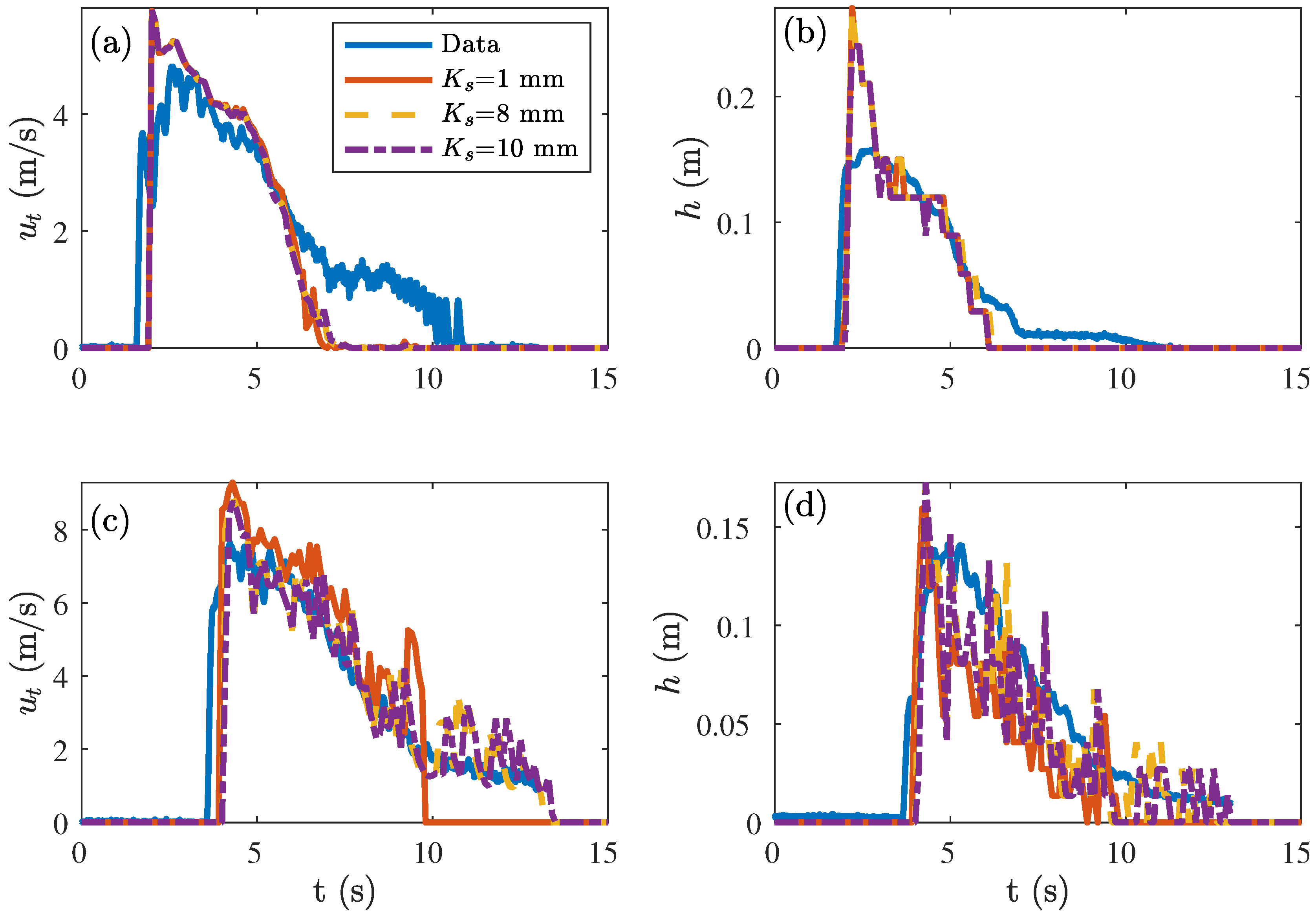
4.2.1. Flow Velocity and Layer Thickness

The model performed well in simulating the maximum flow velocity in the Millingen a/d Rijn case with a dimensionless root-mean-squared error E of 0.09, and the modelled and measured flow velocities were close to the one-one relationship for the 17 overtopping volumes (Figure 6a). The error between the modelled and measured flow velocity was larger for the Vechtdijk case ($E=0.36$) caused by an overestimation of the flow velocity at location V5 for the smaller volumes ($V\le 1$ m${}^3$/m, $U_{max}\le 6.5$ m/s). The same behaviour was observed in the analytical model of Van Bergeijk et al. [12] where the modelled flow velocity was higher on the lower slope compared to the measurements. The modelled flow velocity at V3 showed good agreement with the measured maximum flow velocities. The uncertainty of the measured maximum flow velocity was visible in Vechtdijk for three markers with the same modelled maximum flow velocity, but a different measured flow velocity. These variations were caused by small differences in the released volumes and varied between 2 and 10% of the measured velocity depending on the volume.

The modelled maximum layer thickness was of the same magnitude as the measurements with a normalized root-mean-squared error of 1.08 for Millingen a/d Rijn and 0.28 for Vechtdijk (Figure 6). For Millingen a/d Rijn, the model simulated a sharp peak in the layer thickness at the wavefront (Figure 5b,d) resulting in a higher maximum layer thickness compared to the measurements. The modelled layer thickness over time for the Vechtdijk case (Figure 7b) showed that the peak at the wave front was smaller compared to the Millingen a/d Rijn case (Figure 5b). The difference in peak height at the wavefront could be an explanation for why the layer thickness was overestimated in the Millingen a/d Rijn case and underestimated in the Vechtdijk case. Other explanations for the discrepancy between the modelled and measured were related to the model output parameter $\alpha$, which needed to be translated to a layer thickness. In case a cell was filled with more than 60% of water, the layer thickness was set to the top of the cell. This could lead to an overprediction of 40% of the cell height, which was an error of 1.2 cm for Millingen a/d Rijn and 0.8 cm for Vechtdijk. Finally, the measured maximum layer thickness was influenced by the height on which the surfboard was mounted [26]; Thus, small discrepancies between the modelled and measured maximum layer thickness were expected.

The model was able to predict the decay of the layer thickness and flow velocity accurately, although the wave overtopping period looked smaller because the layer thickness was set to zero when the bottom cell contained less than 60% of water. The model results and measurements reached the second cell in the model around the same time, which was at a height of 4 cm around 6 s in the Vechtdijk case (Figure 7b) and 6 cm around 5.5 s for the Millingen a/d Rijn case (Figure 5b).

The measured and modelled flow velocity and layer thickness showed irregularities over time, which became more pronounced further down the slope due to spreading of the wave (Figure 5 and Figure 7). These irregularities were also observed during overtopping tests on grass-covered dikes (Figure 8b) and flume tests [36]; thus, the model output realistically represented the physics of the overtopping flow. These irregularities were a physical phenomenon related to the roughness of grass, which slowed down the bottom layer of the overtopping wave, but did not affect the top layer. The layer thickness needed to be large enough to overcome the friction of the grass, resulting in fragmented flow down the slope (Figure 8). This illustrated the strength of the model to model this physical process accurately from a linear wave with no irregularities at the boundary of Vechtdijk (Figure 1b) to fragmented flow on the slope.

4.2.2. Vertical Flow Structure

The modelled flow velocity compared well with the measured flow velocity in the top layer for the Vechtdijk case with an overtopping volume of $V=1$ m${}^3$/m. (Figure 9). The exact height of the measured flow velocity near the dike surface was unknown, but the measured flow velocity was of the same magnitude as the modelled flow velocity in the two bottom cells. The modelled vertical flow structure showed excellent agreement with the theoretical law of the wall using $z_0=2.67\times {10}^{-4}\mathrm{m}$ (Equation (15)) and $u_{\tau }=0.3$ m/s [35]. Therefore, we concluded that the structure of the boundary layer was captured well by the model and the numerical model was able to simulate the vertical flow structure accurately.

4.2.3. Pressure

The modelled maximum pressure $p_{max}$ was close to the one-to-one relationship for both measurement locations of Millingen a/d Rijn (Figure 10a). The increase in maximum pressure along the slope from P1 to P2 was simulated well in the model. The points at P1 showed more variation because at this location, a wide range of volumes was available for validation. The markers of P2 corresponding to large overtopping volumes ($V=$ 3–5 m${}^3$/m) compared well with the measurements showing that the model was able to simulate the maximum pressure for these large overtopping volumes accurately. This is also observed in Figure 10b where the modelled pressure p shows the same behaviour over time as the measured pressure for an overtopping volume $V=3$ m${}^3$/m.

4.3. Model Output Potential for Hydraulic Forces during Overtopping

The hydraulic forces in models for grass-cover failure are based on the maximum flow velocity [2,7], the shear stress [2] and the normal stress [15]. These models are categorised into two loading mechanisms: shear forces and normal forces. The shear force mechanism is related to the overtopping flow pulling horizontally on the cover due to high (shear) velocities and turbulence, as described by the maximum flow velocity and shear stress. The overtopping flow pulls vertically during the normal force mechanism leading to under pressures in the sod layer and lifting of the grass cover. The output of this new hydrodynamic model calculates the normal and shear forces on the dike surface covering both loading mechanisms.

The maximum pressure increases at geometrical transitions such as the transitions from the crest to slope due to wave impact, the inner toe due to jet forming and vertical objects and side wall structures due to blockage of the flow [25]. The maximum pressure on the dike surface can be computed with this new model to study the effect of geometrical transitions that are uniform in the along-dike direction. A 3D model is required to calculate the forces along vertical objects and side wall structures.

This section describes the maximum flow velocity, maximum shear stress, maximum normal stress and maximum pressure along the dike profiles of Millingen a/d Rijn and Vechtdijk to show the practical application of the model output for failure of the dike cover.

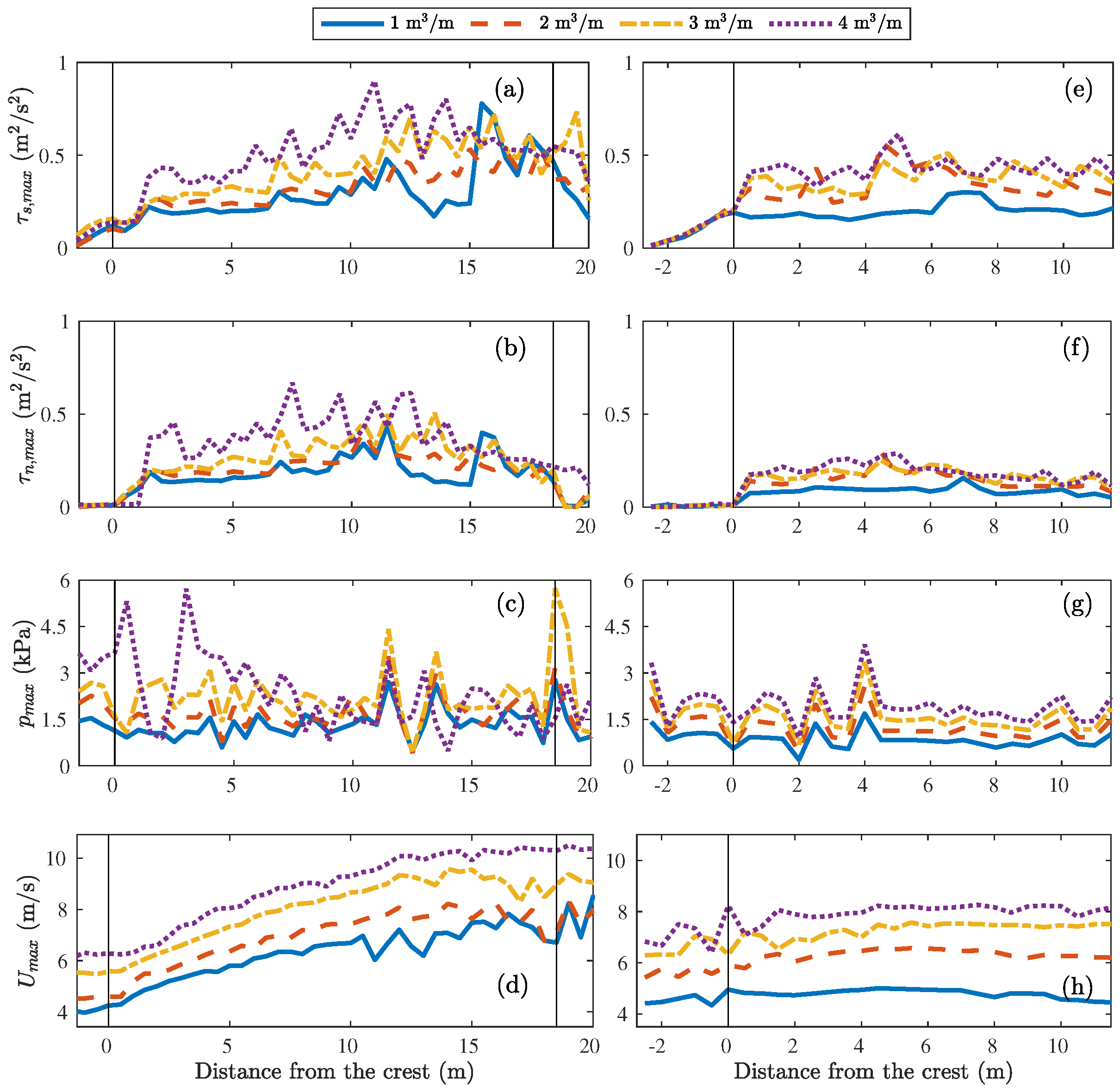
4.3.1. Flow Velocity

The maximum flow velocity increased along the slope for all overtopping volumes in the Millingen a/d Rijn case (Figure 11d). The acceleration along the slope was smaller for the Vechtdijk case, and the flow velocity showed a small decrease around 7 m from the crest for the overtopping volumes $V=1$ m${}^3$/m and $V=2$ m${}^3$/m (Figure 11h). The flow velocity increased until a balance was reached between the gravitational acceleration and bottom friction. The effect of friction became larger when the overtopping wave spread on the slope, which could lead to a decrease in flow velocity. The flow velocity did not decrease for the larger volumes because the effect of friction was relatively smaller for larger overtopping volumes.

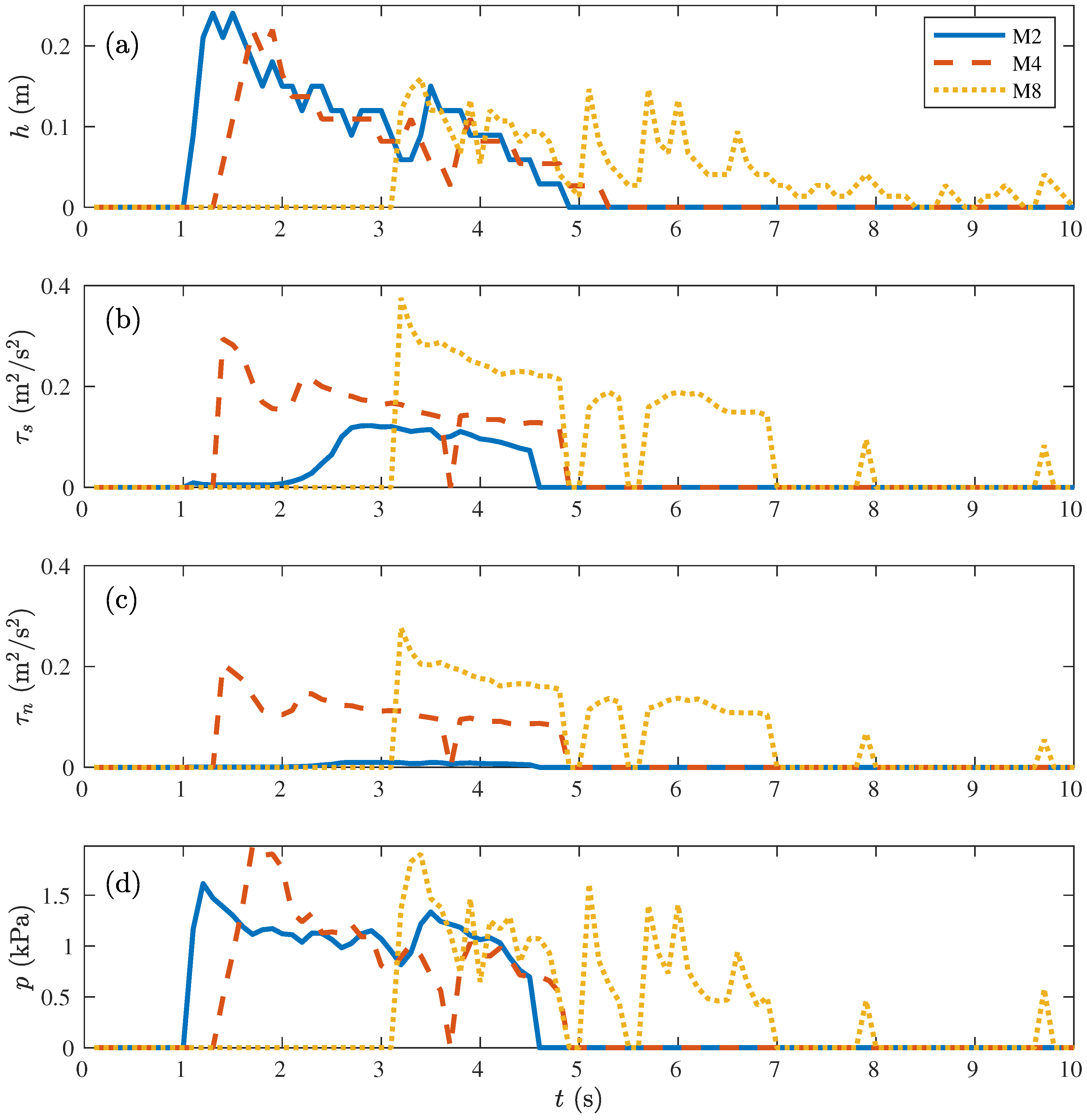
4.3.2. Shear and Normal Stress

The shear stress ${\tau }_s$ and the normal stress ${\tau }_n$ varied both in time and space (Figure 12b,c). The maximum shear and normal stress occurred at the wave front for the locations on the slope (M4 and M8), while the stresses were negligibly small at the wave front on the crest (M2). The shear stress on the crest started to increase in the layer thickness at $t=1.9$ s and $t=3.5$ s related to the fragmented flow as seen in the layer thickness over time (Figure 12a). The normal stress on the crest (M2) was negligibly small. The shear stress and normal stress followed the same behaviour over time on the slope (M4 and M8), but the shear stress was higher than the normal stress at all time steps. For Vechtdijk, the stresses were also maximum at the wave front, and the shear stress was higher than the normal stress at all locations.

The maximum stresses with respect to time varied with the cross-dike location and overtopping volume (Figure 11). The maximum shear stress ${\tau }_{s,max}$ increased with increasing volume, although the maximum shear stress for $V=1$ m${}^3$/m was larger at 16 m from the crest than $V=2$ m${}^3$/m and $V=3$ m${}^3$/m at Millingen a/d Rijn (Figure 11a,e). The maximum stress showed a slow increase over the crest and upper slope for both Millingen a/d Rijn and Vechtdijk. The model domain of Millingen a/d Rijn included the entire landward slope and inner toe—indicated by the vertical line at 18.5 m—showing the increase in maximum shear stress along the slope followed by a slow decrease landward of the inner toe. The maximum shear stress was highest on the lower slope, and the location of the peaks in the maximum shear stress varied with the overtopping volumes. The maximum normal stress ${\tau }_{n,max}$ was approximately zero on the crest followed by a rapid increase around 1–2 m from the crest and decreased to zero at the end of the slope (Figure 11b,f). The normal stress was maximum on the slope, but the exact location again depended on the overtopping volume.

4.3.3. Pressure on the Bed

The modelled pressure on the dike surface was maximum at the wavefront at all measurement locations (Figure 12d). The pressure over time showed more irregularities further down the slope, which was related to the spreading of the overtopping wave as seen in the layer thickness with a longer overtopping period and more irregularities at M8 (Figure 5d) compared to M2 (Figure 5b). The pressure for the Vechtdijk case showed the same behaviour over time, with the maximum pressure at the wave front and more irregularities in the shape at the end of the model domain.

The maximum pressure $p_{max}$ with respect to time was largest at the start of the dike crest, contrary to the maximum shear and normal stress, and around 4 m from the crest for the Vechtdijk case (Figure 11g). For the Millingen a/d Rijn case, peaks in the maximum pressure were observed at the start of the slope, on the lower slope and at the inner toe. The maximum pressure showed the same cross-dike behaviour for all overtopping volumes in the Vechtdijk case, while for the Millingen a/d Rijn case, the behaviour was similar for $V=$ 1–3 m${}^3$/m. The maximum pressure increased with increasing volume, although the maximum pressure of $V=3$ m${}^3$/m was larger than $V=4$ m${}^3$/m at the inner toe for the Millingen a/d Rijn case.

A peak in the maximum pressure was observed at the inner toe of Millingen a/d Rijn for all overtopping volumes, which was especially clear for $V=3$ m${}^3$/m, where the maximum pressure doubled at the inner toe. This showed the ability of the model to quantify the location and the increase in maximum pressure at geometrical transitions.

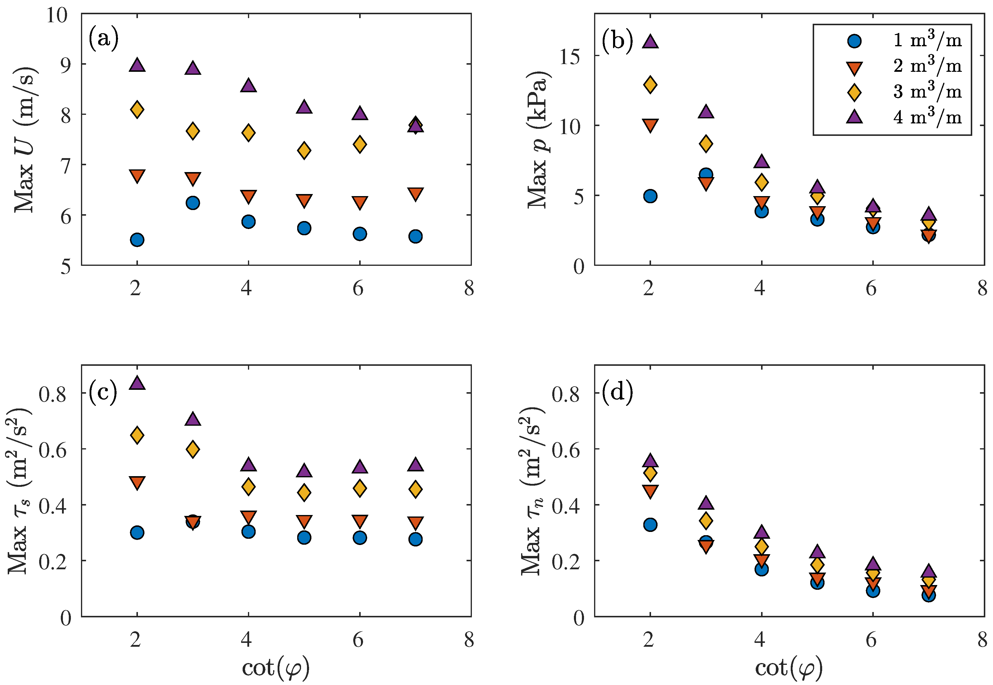
4.4. The Effect of the Slope Steepness

The hydraulic forces on a grass-covered dike were modelled for varying the steepness of the landward slope to show the effect of geometry on the hydraulic forces. The maximum flow velocity, pressure, shear stress and normal stress with respect to time and space were calculated for six values of slope steepness $cot\left(\phi \right)$ and four overtopping volumes. The same boundary conditions as the Vechtdijk case were used and the dike height and crest width were set to 5 m and 2 m, respectively.

All four variables increased with increasing overtopping volume and steepening of the slope, corresponding to a decrease in the slope steepness $cot\phi$ (Figure 13). The normal stress was most sensitive for the slope steepness, leading to more than doubling of the normal force with a increase in steepness from $cot\left(\phi \right)=8$ to $cot\left(\phi \right)=3$ (see

Table A1. Comparison of the relative increase in the hydraulic variables with increasing volume V for $cot\left(\phi \right)=3$ and with increasing slope steepness $cot\left(\phi \right)$ for $V=1$ m${}^3$/m for a simple grass-covered dike with a dike height of 5 m and a crest width of 2 m.

	Increase from $\mathit{V}=1$ m${}^3$/m to $\mathit{V}=4$ m${}^3$/m	Increase from $cot\left(\mathit{\phi }\right)=8$ to $cot\left(\mathit{\phi }\right)=3$
Flow Velocity	42%	13%
Pressure	84%	168%
Shear Stress	106%	21%
Normal Stress	53%	225%

in Appendix A for the exact numbers). The pressure also increased significantly with increasing steepness, while the increase was relatively smaller for the shear stress and the flow velocity. The shear stress changed for a steepness of $cot\left(\phi \right)=2$ and $cot\left(\phi \right)=3$, but was approximately constant for $cot\left(\phi \right)=$ 4–8. However, the flow velocity and shear stress were affected more by the overtopping volume compared to the pressure and normal stress.

The flow velocity, pressure and shear stress were smaller for a steepness $cot\left(\phi \right)=2$, compared to $cot\left(\phi \right)=3$ for $V=1$ m${}^3$/m. In this case, the length of the slope for $cot\left(\phi \right)=2$ was too short to gain the same amount of acceleration as on the longer slope of $cot\left(\phi \right)=3$. As mentioned before, the acceleration was volume dependent; thus, this effect was smaller for the other overtopping volumes.

5. Discussion

5.1. Model Application and Limitation

The numerical model developed in this study showed good agreement with the measurements and provided a wide range of output variables including the hydraulic forces on the cover. The boundary conditions could be generated using the overtopping volume, and the mesh was easily generated from a few GPS measurements of the dike profile. The model is generally applicable to a variety of dike profiles, also for irregular profiles. Small irregularities of the grass cover were captured in the roughness height in the turbulence model, and larger irregularities such as erosion holes and large bumps needed to be resolved in the mesh, for example the bump at the toe of Millingen a/d Rijn at $x=$ 20–22 m in Figure 2. The model was computationally fast with a maximum run time of 20 min in the two studied cases.

The model results became less reliable for small layer thicknesses that were smaller than or equal to the vertical grid size. The wetting and drying of the cells for such layer thicknesses resulted in high values of the stresses in the tail of the wave contrary to other studies that only predicted high stresses at the wave front [2,5]. The cells were quite course with heights of 2–3 cm. Smaller cells would improve the model results for small layer thickness, but at the same time, this would significantly increase the computational time.

The effect of turbulence on the hydraulic forces was incorporated into the model using the $k-\omega$ SST turbulence model. However, the pressure and velocity fluctuations related to small scale turbulent processes were not directly modelled, as is done in direct numerical simulations (DNS).

The model application is limited to flood defences with maintained grass covers, as discussed in more detail in Section 5.2. However, these grass-covered flood defences are located across the world including the USA [3] and China [14] making the research internationally relevant. Moreover, grass-covered flood defences are becoming more popular to increase the ecological value of the flood defences [37].

The major advantage of this new model compared to the other models is that the output covers the flow velocity, pressure, normal and shear stress. This means that the load does not need to be calculated for every erosion model separately, but the model output can be used to calculate several failure mechanisms of the dike cover. Locations with high hydraulic loads can be identified because the hydraulic load is computed along the dike crest and landward slope. It is important to identify vulnerable locations for dike failure and to understand why the dike fails at these locations. For example, the flow velocity and shear stress were maximum at the end of the slope of the Millingen a/d Rijn case, making the lower slope a vulnerable location for failure due to the shear force mechanisms. The normal stress was maximum halfway of the slope, which was a vulnerable location for failure by the normal force mechanisms. Peaks in the pressure were observed at multiple locations along the dike profile including the inner toe and the start and end of the dike crest. At these locations, the geometry changed making them vulnerable to cover failure due to wave impact or jet forming. Until now, it is unknown when and where wave impact, jet forming or other loads will occur. This new numerical model could be used to investigate which hydraulic loads, such as overtopping volumes, and at which locations along different dike geometries the various failure mechanisms would develop.

The model was applied to a dike with varying slope steepness and four overtopping volumes to show the effect of dike geometry and varying load on the hydraulic forces. Relationships between the hydraulic forces—maximum flow velocity, pressure, shear stress and normal stress—and important variables such as the overtopping volume and slope steepness could be derived to provide a quick estimation of the maximum hydraulic forces on a grass-covered defences. This requires determining all important variables that affect the hydraulic forces, which are not solely determined by the slope steepness and overtopping volume, but by the crest width, dike height and cover type as well. Thorough investigation of the effect of all variables on the hydraulic forces is required to obtain such relationships, which is outside the scope of this paper, which is mainly focused on calculating the forces along the dike profile and identifying locations where the forces are large.

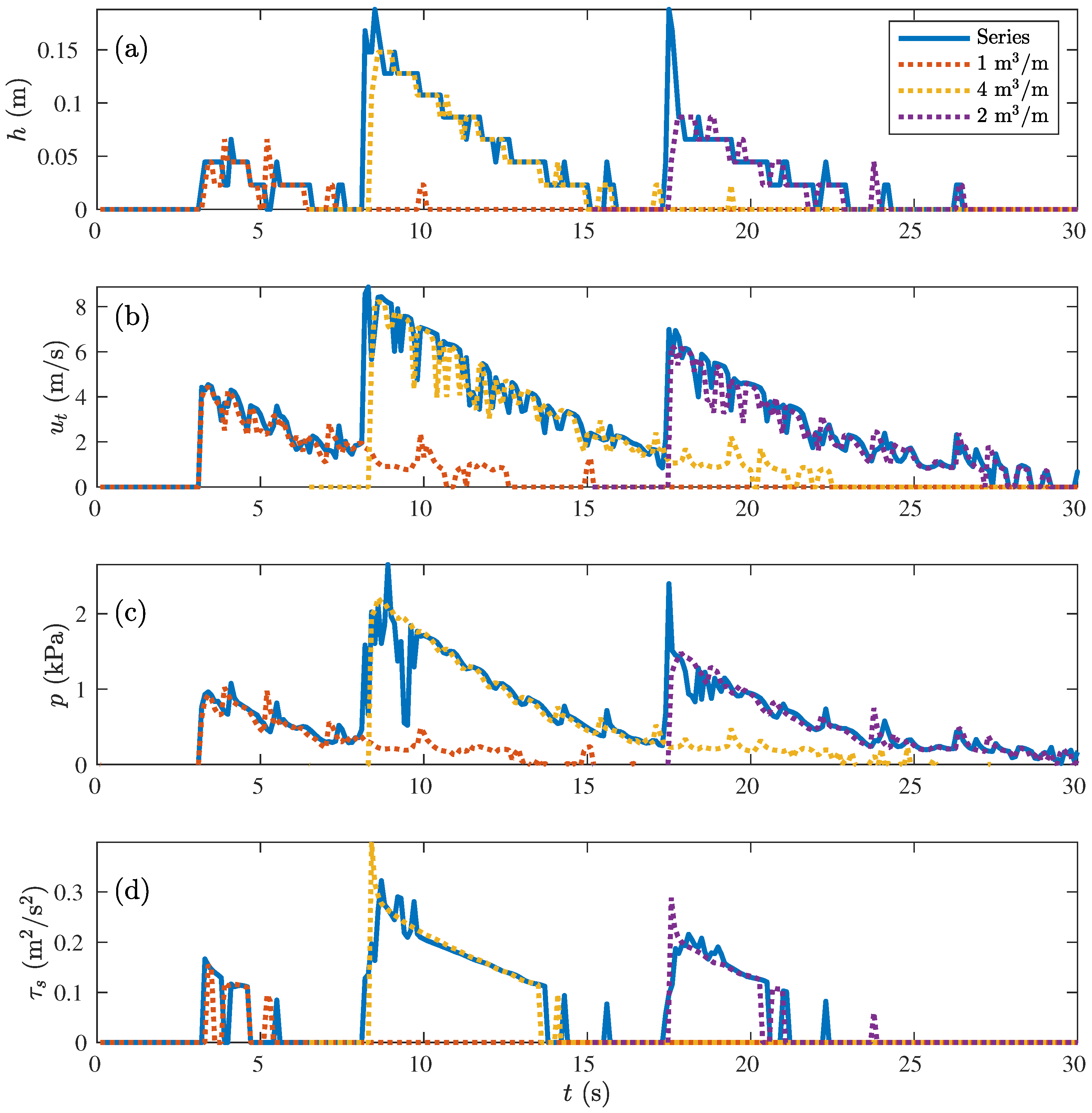
Individual Overtopping Volumes

Only individual overtopping waves were simulated in this study, but these volumes can be used to simulate wave overtopping during a storm. A distribution of overtopping wave volumes based on the wave height and storm duration was generated to simulate the amount of wave overtopping during storm and determine failure or the amount of erosion during this storm [6,7,38]. It is possible to simulate all the overtopping waves during a storm—between zero and 5000 waves depending on the overtopping discharge—with empirical or analytical formulas [7,38]. Simulating all waves overtopping during a storm takes much more computational power when CFD models are used. For that reason, Bomers et al. [6] discretized the volume distribution into five representative overtopping volumes to simulate the erosion during a storm. Thus, individual overtopping volumes as modelled in this study are representative for overtopping in real situations once combined with a volume distribution.

The overtopping waves on the crest were identified as individual overtopping volumes because only the highest waves during a storm overtop the dike [10]. Although the overtopping volumes during a storm are separated on the crest, larger volumes accelerate more on the slope compared to smaller volumes, which means that large volumes can overtake and combine with a small volume on the landward slope. Additionally, when simulating solely the individual volumes, it was assumed that the slope was completely dry before the wave overtops. However, the grass cover does not completely dry after every overtopping wave, and there is always some water left on the crest due to friction.

To study the effect of both processes, a time series of three overtopping waves was simulated for the Vechtdijk case with overtopping volumes of 1 m${}^3$/m, 4 m${}^3$/m and 2 m${}^3$/m entering the domain with two seconds of spacing. The layer thickness, flow velocity, pressure and shear stress over time at V5 were computed and compared to the model results of the individual overtopping waves in dotted lines at the end of the model domain (Figure 14). A wave taking over the previous overtopping wave was not observed as seen in the layer thickness. This was also not observed during other model runs with a spacing of 1 s or different combinations of waves. However, a small amount of water was left on the slope before the next wave arrived on the slope as seen in the flow velocity and pressure in this small layer ($<0.6\Delta z=1.2$ cm) that were non-zero when the next wave arrived. The remaining water layer of the previous overtopping wave led to an increase of the layer thickness at the wave front for the second and third overtopping waves (Figure 14). This small water layer had no effect on the flow velocity in the top layer, but led to an increase in the maximum pressure at the wave front related to the increase in the layer thickness leading to an increase in the hydrostatic pressure (Equation (12)). The shear stress at the wave front was reduced because the water level reduced the bottom friction. Thus, simulating only individual waves on a dry cover could lead to an underestimation of the maximum layer thickness and maximum pressure at the wave front while the maximum shear stress was slightly overestimated compared to a time series.

The possibility to compute time series and include the effect of the small water layer of the previous overtopping waves on the next overtopping wave showed the power of this new model. It was not possible to include this effect on the existing models for the overtopping flow on the dike crest and the landward slope. It took 23.5 min to simulate 50 s of the time series, which meant that modelling a time series could be more efficient than simulating the individual overtopping waves when the time between the overtopping waves is not too long. Modelling of a time series was not done for the model validation in this study, because only data of individual overtopping waves were available.

5.2. Roughness Height

The Nikuradse roughness height was calibrated to 8 mm for wave overtopping flow over grass-covered dikes. The roughness height was assumed to be uniform along the profile and the same for the Vechtdijk and Millingen a/d Rijn cases. Although the grass type differed between both cases, namely hay grass at Millingen a/d Rijn [39] and meadow grass at Vechtdijk [24], the covers were maintained in the same way. The assumption of uniform roughness for grass-covered dikes was valid since the roughness in the model accounted for both roughnesses of the grass stems as the small variations in height of the dike profile due to irregularities of the grass cover. The latter roughness was dominant over the height of the grass stems, because the grass stems were elastic leading to flatting by the overtopping flow [36]. The model had a vertical grid size of 2–3 cm; thus, the model accounted for the cover roughness of all irregularities within the cell. This meant that the roughness height did not need to be calibrated for other grass covers; however, the roughness height might be different for other vegetation types that result in different type of cover irregularities, such as species-rich covers with herbs [36].

The modelled flow velocity and layer thickness were not sensitive to the roughness height (Figure 5), and no clear relationship between the normalised root-mean-squared error and the roughness height was observed. The roughness height influenced the magnitude of the shear and normal stresses through the effective viscosity ${\nu }_{eff}$. No measurements of the stress due to overtopping waves on grass-covered dikes were available; thus, this variable could not be used for calibration of the roughness height. A difference in magnitude of the shear stress had no influence on the failure or erosion of the grass cover, because both were calculated using the exceedance of a critical stress. The value of the critical stress is model dependent and needs to be calibrated for this new model. A higher critical stress related to a higher roughness height would result in the same amount of erosion as a smaller critical shear stress for a small roughness height. The location where the dike would fail was related to the location of maximum shear stress. The maximum shear stress occurred at the wave front, which was not sensitive to the roughness height with a shift of less than 0.5 m between $K_s=1$ mm and $K_s=10$ mm. The roughness height had more effect on the tail of the wave; hence, it is advised to investigate the effect of roughness for processes that are important in the tail of the wave.

The calibrated roughness height corresponds to a roughness constant for uniform closely packed sand grains ($C_s=0.5$). A grass cover consists of non-uniform roughness elements with different spacing, so the value of $C_s$ can be very different for this cover. However, we assumed $C_s=0.5$ because the value of $C_s$ is unknown for grass cover. A different value for the constant $C_s$ resulted in a different value of $K_s$, which is shown in

Table 3. The root-mean squared error between the modelled and measured maximum flow velocity of Millingen a/d Rijn in m/s for an overtopping volume of 2.5 m${}^3$/m as a function of the roughness height $K_s$ and three values of the roughness constant $C_s$ where the bold values correspond to the lowest error per roughness constant.

${\mathit{K}}_{\mathit{s}}$ (mm)	1	2	3	4	5	6	7	8	9	10
$C_s=0.1$	0.92	0.88	0.88	0.88	0.90	0.87	0.89	0.96	0.86	0.87
$C_s=0.5$	0.38	0.60	0.68	0.53	0.44	0.41	0.43	0.51	0.60	0.65
$C_s=0.9$	0.86	0.82	0.81	0.81	0.82	1.05	0.89	0.91	0.92	1.09

for the root-mean-squared error between the modelled and maximum flow velocity of $V=2.5$ m${}^3$/m in the Millingen a/d Rijn case. The smallest error occurred for a roughness height of 9 mm, 1 mm and 3–4 mm for a roughness constant of 0.1, 0.5 and 0.9, respectively. The error was smallest for $C_s=0.5$ for all roughness heights indicating that this setting was most suitable for modelling grass roughness. No clear minimum in the error was observed for $C_s=0.1$ and $C_s=0.9$, indicating again an insensitivity of the model to the roughness height.

Assuming a $C_s$ value of 0.5, the calibrated value of the Nikuradse roughness height could be transferred to the Manning’s coefficient n for comparison with the literature values of Chow [40]:

$$n=0.0391K_s^{1/6}=0.0175$$

(16)

which was close to $n=$ 0.025–0.035 for grass in floodplains and $n=$ 0.022–0.033 for uniform earthen channels with short grass.

The calibrated roughness values were model specific; thus, it was expected that the roughness height varied between numerical studies. The numerical study of Bomers et al. [6] used a roughness height of 6.8 cm for grass and 2.1 cm for clay based on literature values [25,40]. However, both values were much larger than the grid size of 2.3 mm in the numerical model of Bomers et al. [6], which means that the roughness height loses its physical meaning. This could also be an indication of the insensitivity of the model to the roughness height as observed in this study. Moreover, the roughness height of 6.8 cm was calculated from a calibrated value of the friction factor for grass in an analytical model for the maximum flow velocity [25]. This model specific roughness height could not be used in numerical models without validation, just like the calibrated roughness height of 8 mm in our study was not applicable to other numerical models. This was because the roughness is part of the turbulence model in such a manner that a different turbulence model could result in a different roughness value. Roughness is not only model specific, but also depends on the flow characteristics, which differ between flow types such as unsteady overtopping flow and steady overflow.

5.3. Comparison with Existing Modelling Approaches

This new numerical model was developed to calculate the hydraulic forces along flood defences with a grass-covered crest and landward slope. The modelled hydraulic forces included the maximum flow velocity, shear stress, normal stress and pressure. The pressures on hard structures during wave overtopping were simulated in other numerical studies to determine the forces on breakwaters [16,18] or sea walls [20]. The forces were calculated from the integration of the pressure over the impact duration and focussed on structural failure, which meant that the normal and shear stress were not determined in these studies.

However, the normal and shear stresses are important to determine the erosion of the dike cover and failure of grass-covered flood defences [2,15,41]. For that reason, Bomers et al. [6] were the first to determine the shear stress on a grass cover. The shear stress was not obtained from the model output, but calculated from the modelled near bed velocity, which was not validated. In this study, we validated the near bed velocity and showed the model output for the pressure, the shear stress and the normal stress, which could easily be obtained from the model and did not need to be calculated separately.

The numerical model of the Millingen a/d Rijn case included the complete landward slope from the crest to the inner toe, contrary to other studies that only included part of the landward slope [5,6] or the slope was below the still water level [16,18]. This made it possible to study the forces on the dike cover at the inner toe, which is an important location where often the grass cover fails due to jet forming [42].

Our numerical model was computationally fast because of the new boundary conditions limiting the model domain to only the crest and landward slope of the flood defence. The generation of the waves and modelling the wave run-up took a lot of computational time in the other numerical models [16,18,20]. The model domain of Bomers et al. [6] started in the overtopping simulator on the crest, which meant that the model was not generally applicable. Our new boundary conditions made it possible to simulate the hydraulic forces on the cover in detail with low computational costs. It is also possible to couple our model to other numerical overtopping models that end at the crest through the modelled flow velocity and layer thickness as in the Millingen a/d Rijn case or through individual overtopping volumes as in the Vechtdijk case.

5.4. Sensitivity of the Model Settings

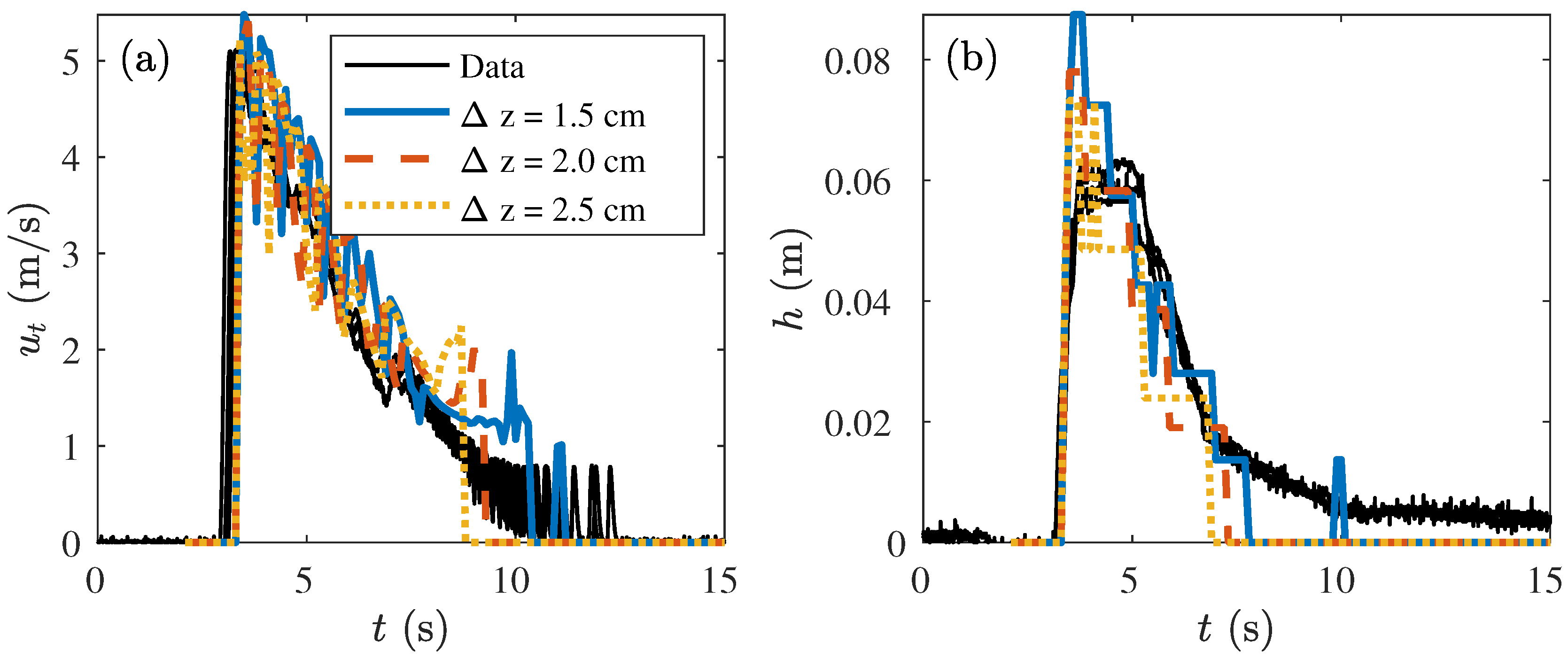
5.4.1. The Layer Thickness

The layer thickness was not a model output variable, but was calculated from the water fraction $\alpha$ (Section 3.1.2). The layer thickness was set to the highest cell that contained more than 60% of water ($\alpha >0.6$). The flow velocity in the top layer—defined as the flow velocity at height $z=h$—was also related to the water fraction $\alpha$ through the layer thickness. The maximum modelled flow velocity and layer thickness were determined for three thresholds of the water fraction $\alpha$ (see Figure A1 in Appendix B). Small changes in the maximum flow velocity and layer thickness were observed; however, changing the threshold of $\alpha$ for the layer thickness had no significant effect on the model results.

5.4.2. The Near Bed Velocity

The near bed velocity measured 2–3 cm from the dike surfaces was compared to the modelled velocity in the centroid of the second cell from the bottom. Comparison of the measured maximum flow velocity near the bed at M3, M5 and M7 with the modelled maximum flow velocity in the centroid of the first, second and third cell showed that the modelled flow velocity increased from the first till the third cell as expected in the boundary layer (Figure 15). The measured near bed velocity compared well with the modelled flow velocity in Cells 2 and 3, but was higher than the flow velocity in Cell 1. For that reason, the measured near bed velocities at M3, M5, M7 and V3 were compared to the modelled flow velocity in Cell 2 instead of Cell 1 (Section 3.1.2). According to the field test reports [24,25], the near bed velocity was measured 2–3 cm from the dike surface, which was closer to the centroid of the first cell at 1.5 cm compared to the centroid of the second cell at 4.5 cm for the Millingen a/d Rijn case. However, the flow velocity in the first cell might be affected too much by the wall functions in the turbulence model or the paddle wheels on the bed did not measure the real near bed velocity, but the flow velocity a little higher up in the flow resulting in a better agreement with the flow velocity in the second cell.

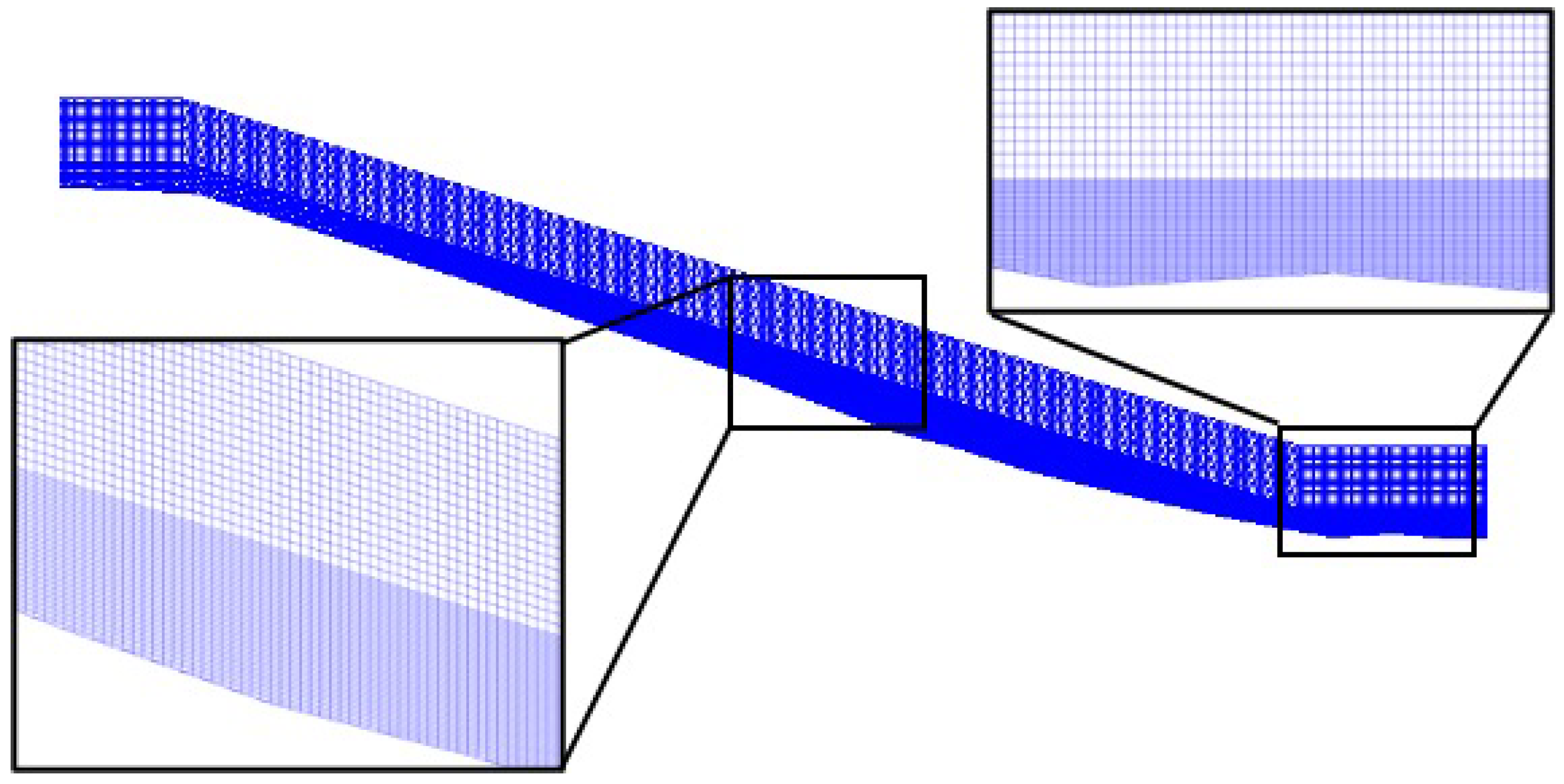
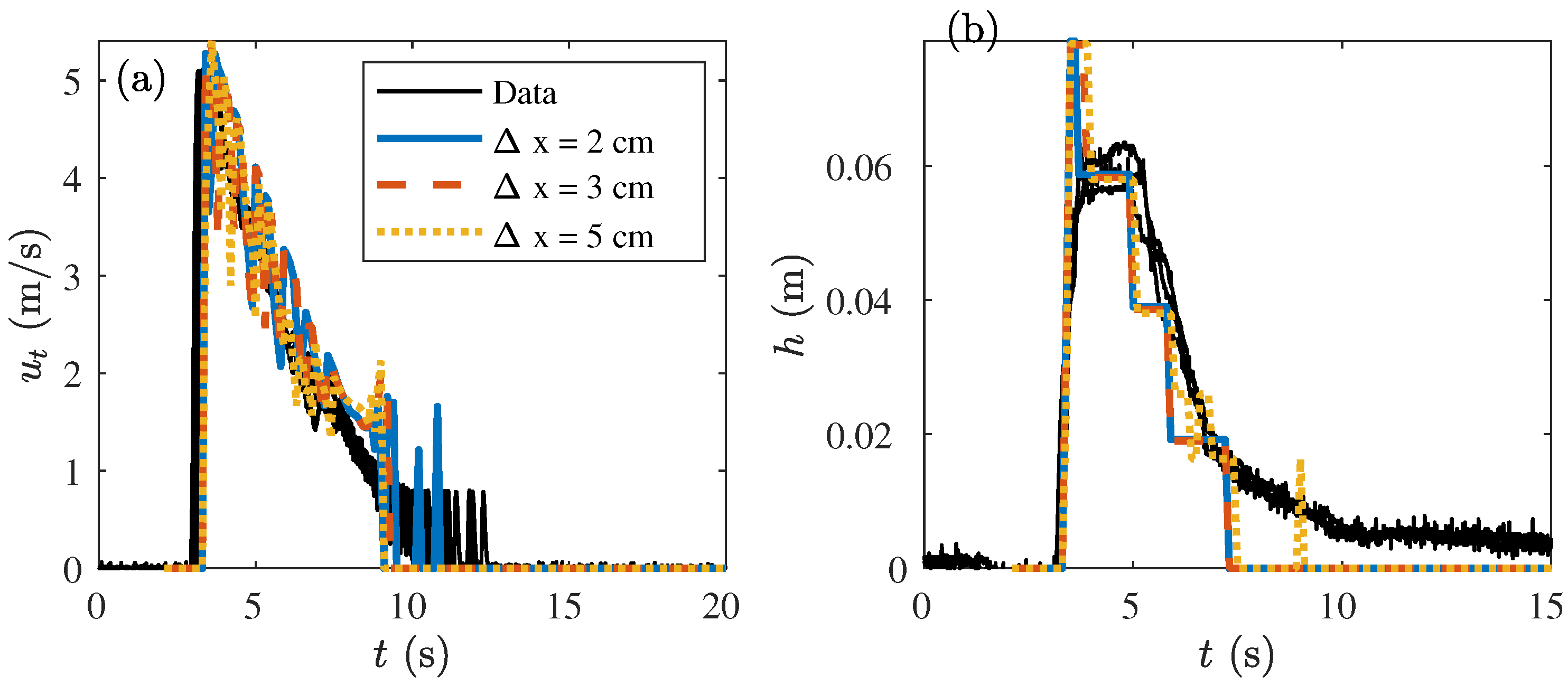
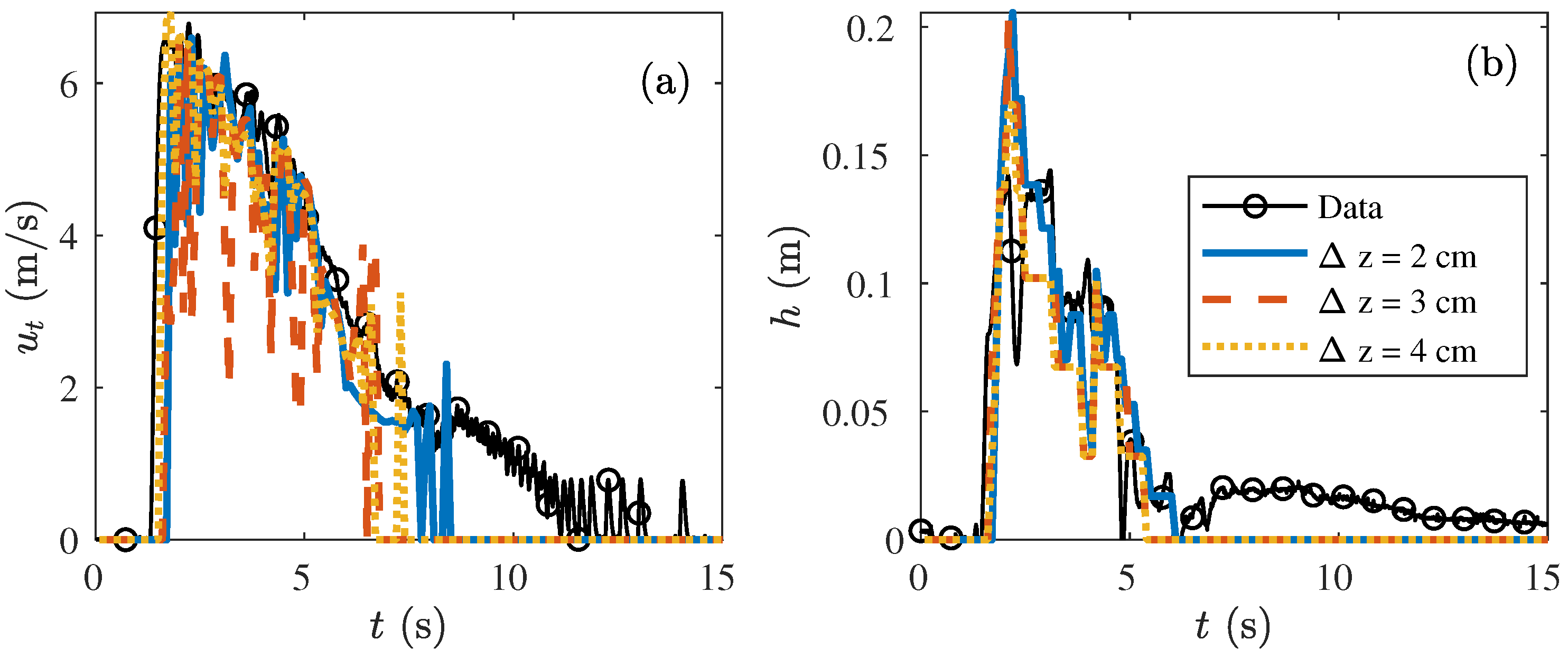
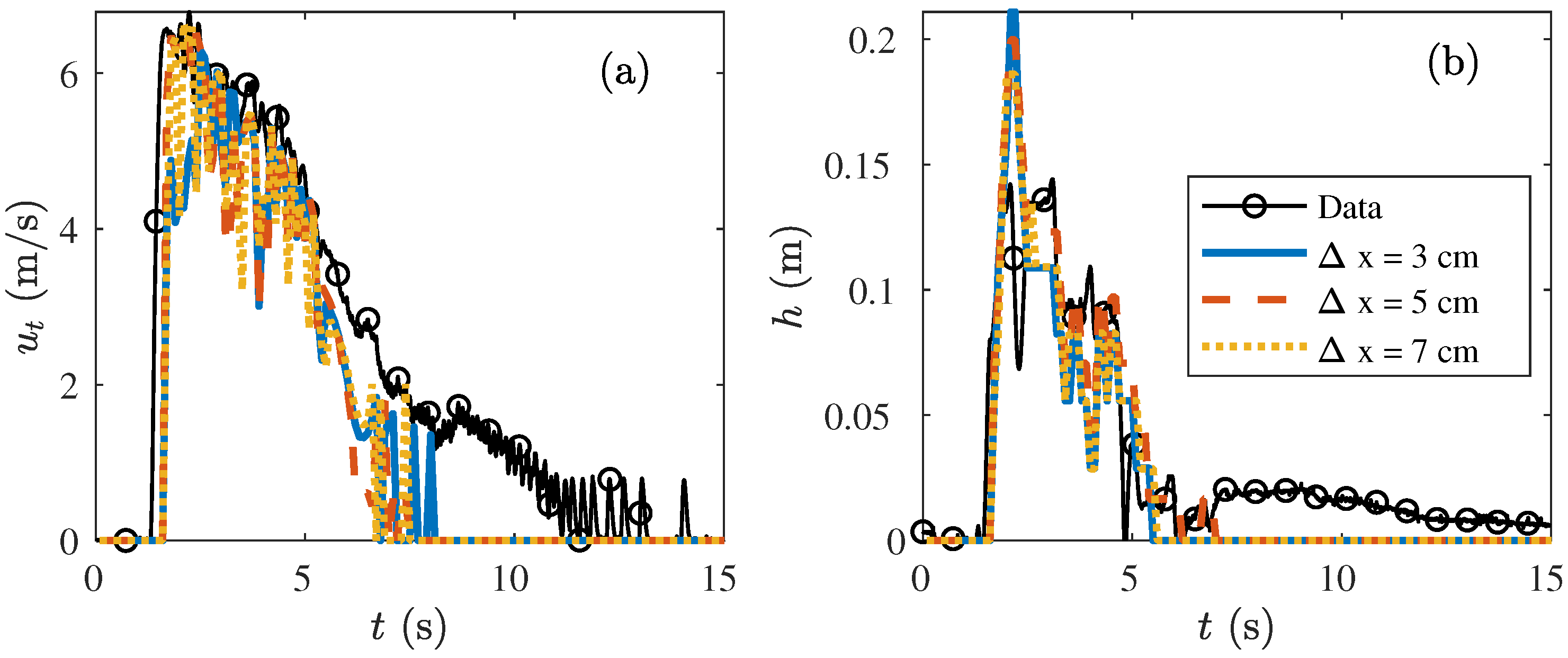
5.4.3. The Effect of the Grid Size

Multiple model runs with different grid sizes were performed for both the Vechtdijk and the Millingen a/d Rijn case (

Table 4. The effect of the horizontal grid size $\Delta x$ and the vertical grid size $\Delta z$ on the computational time and the observed maximum flow velocity $U_{max,o}$ and modelled maximum flow velocity $U_{max,m}$ at V3 and M6 for Vechtdijk and Millingen a/d Rijn, respectively.

Profile	$\mathbf{\Delta }\mathit{x}$ (cm)	$\mathbf{\Delta }\mathit{z}$ (cm)	Time (min)	${\mathit{U}}_{\mathit{max}}$ (m/s)
Vechtdijk 1 m${}^3$/m $U_{max,o}=5.12$ m/s	3.0	2.0	17.4	5.41
	3.0	1.5	23.3	5.44
	3.0	2.5	9.0	5.19
	2.0	2.0	32.3	5.50
	5.0	2.0	5.3	5.37
Millingen a/d Rijn 2.5 m${}^3$/m $U_{max,0}=6.78$ m/s	5.0	3.0	13.5	6.52
	5.0	2.0	18.2	6.59
	5.0	4.0	13.0	6.93
	3.0	3.0	20.0	6.29
	7.0	3.0	5.2	6.64

). The differences between the model runs were small showing that the model results were not affected by the grid size. The difference between the modelled and measured maximum flow velocity was smaller than 7% for all model runs (Table 4). The grid size had a small effect on the overtopping period. A smaller vertical grid size $\Delta z$ led to a slight increase in the overtopping period (see figures in the Appendix B). The horizontal grid size also affected the overtopping period, but no clear relation was observed.

The layer thickness at the wave front needed to be at least two vertical cells to resolve the shear velocity near the bed and the flow velocity in the top layer of flow. However, the model results improved significantly when three vertical cells were wetted at the start of the wave front. In this study, the vertical grid size was constant for all modelled volumes, but we advise to adapt the grid size for the overtopping volume. In that case, a smaller grid size was required for modelling an overtopping volume of 0.4 m${}^3$/m where only two cells were wetted at the wavefront. The vertical grid size could be increased for overtopping volumes larger than 2 m${}^3$/m to decrease the computational time, but more wetted cells increased the accuracy of the modelled boundary layer, for example five cells at the wave front, as in Figure 9.

6. Conclusions

The goal of this study was to develop a detailed hydrodynamic model to simulate the overtopping flow along the grass-covered crest and landward slope of a flood defence to determine the temporal and spatial variation in the hydraulic load. This new numerical model could calculate the high loads caused by (1) high flow velocities at the wave front, (2) wave impact at geometrical changes and (3) turbulence leading to high stresses. This numerical model was the first model for overtopping flow on grass-covered flood defences that captured these important processes necessary to determine the location and magnitude of the hydraulic forces. The model proved able to calculate the near bed velocity, the pressure, the shear stress and the normal stress on the cover of the overtopping wave along the profile.

The model was shown to perform well for two validation datasets of field tests on grass-covered dikes in the Netherlands. The maximum modelled flow velocity compared well to the measurements with maximum flow velocities of 9.2 m/s and 9.1 m/s for Millingen a/d Rijn and Vechtdijk, respectively. The model captured the vertical flow structure and showed good agreement with the measurements of the flow velocity in the top layer and near the bed, as well as the theoretical logarithmic wall function. The shear stress was maximal on the lower slope, while the normal stress was maximal halfway of the slope. The pressure was maximal on the dike crest and at the inner toe. The stresses and pressure increased with increasing overtopping volume, but the maximum stresses showed more variability with varying volumes compared to the pressure. The output variables were all maximal at the wave front; thus, it is was important to simulate the wave front correctly.

The numerical model was applied to a grass-covered dike with different values of the slope steepness on the landward side. The slope steepness had a large effect on the modelled variables with a large increase in the magnitude of the pressure and more than doubling of the magnitude of the normal stress when the slope changed from 1:8 to 1:3. The overtopping volume had a larger effect on the shear stress compared to the slope changes. The magnitude of the maximum normal stress and the maximum pressure was only slightly affected by the overtopping volume, but the locations of the maximal forces changed with the overtopping volume. Therefore, it is important to not only compute the forces along the dike profile, but also simulate as many volumes as possible during a storm.

This numerical model could quantify the location and the magnitude of the hydraulic forces along the dike crest and landward slope. Vulnerable locations for cover erosion were identified at the lower slope due to high shear forces and halfway of the slope related to the a high normal forces. Additionally, high pressures were modelled at geometric transitions with a doubling of the maximum pressure at the inner toe. This study was the first to quantify this pressure increase because the model domain of Millingen a/d Rijn included the entire landward slope including the horizontal part landward of the inner toe. The model was computationally fast due to the relatively large grid size and new boundary conditions based on individual overtopping volumes.

Accurate simulations of the hydraulic forces along the dike profile could help to improve the design and assessment of grass-covered flood defences. The modelled hydraulic forces were important variables to determine the location and amount of cover erosion and failure of grass-covered flood defences. The temporal variation in the model output variables was essential to determine the amount of erosion, while the spatial variation could be used to find vulnerable spots of the flood defences.

References

1. Van der Meer, J.W.; Allsop, N.W.H.; Bruce, T.; De Rouck, J.; Kortenhaus, A.; Pullen, T.; Schüttrumpf, H.; Troch, P.; Zanuttigh, B. Manual on Wave Overtopping of Sea Defences and Related Structures. An oVertopping Manual Largely Based on European Research, But for wOrldwide Application; Technical Report; EurOtop: London, UK, 2018; Available online: www.overtopping-manual.com (accessed on 28 February 2019).
2. Hoffmans, G.J.C.M. The Influence of Turbulence on Soil Erosion; Eburon Uitgeverij BV: Utrecht, The Netherlands, 2012. [Google Scholar]
3. Hughes, S.A. Adaptation of the Levee Erosional Equivalence Method for the Hurricane Storm Damage Risk Reduction System (HSDRRS); Technical Report; U.S. Army Corps of Engineers: New Orleans, LA, USA, 2011. [Google Scholar]
4. Van der Meer, J.W. Erosion Strength of Inner Slopes of Dikes Against Wave Overtopping. Preliminary Conclusions after Two Years of Testing with the Wave Overtopping Simulator; Summary Report; Van der Meer Consulting: Akkrum, The Netherlands, 2008. [Google Scholar]
5. Aguilar-López, J.P.; Warmink, J.J.; Bomers, A.; Schielen, R.M.J.; Hulscher, S.J. Failure of grass covered flood defences with roads on top due to wave overtopping: A probabilistic assessment method. J. Mar. Sci. Eng. 2018, 6, 74. [Google Scholar] [CrossRef] [Green Version]
6. Bomers, A.; Aguilar-López, J.P.; Warmink, J.J.; Hulscher, S.J. Modelling effects of an asphalt road at a dike crest on dike cover erosion onset during wave overtopping. Nat. Hazards 2018, 93, 1–30. [Google Scholar] [CrossRef] [Green Version]
7. Van der Meer, J.W.; Hardeman, B.; Steendam, G.J.; Schüttrumpf, H.; Verheij, H. Flow depths and velocities at crest and landward slope of a dike, in theory and with the wave overtopping simulator. Coast. Eng. Proc. 2010, 1, 10. [Google Scholar] [CrossRef] [Green Version]
8. Van Gent, M.R.A. Low-Exceedance Wave Overtopping Events: Estimates of Wave Overtopping Parameters at the Crest and Landward Side of Dikes; Delft Cluster: Delft, The Netherlands, 2002. [Google Scholar] [CrossRef] [Green Version]
9. Schüttrumpf, H.; Oumeraci, H. Layer thicknesses and velocities of wave overtopping flow at seadikes. Coast. Eng. 2005, 52, 473–495. [Google Scholar] [CrossRef]
10. Hughes, S.A.; Thornton, C.I.; Van der Meer, J.W.; Scholl, B.N. Improvements in Describing Wave Overtopping Processes. Coast. Eng. Proc. 2012, 1, 35. [Google Scholar] [CrossRef]
11. Van Damme, M. Distributions for wave overtopping parameters for stress strength analyses on flood embankments. Coast. Eng. 2016, 116, 195–206. [Google Scholar] [CrossRef] [Green Version]
12. Van Bergeijk, V.M.; Warmink, J.J.; Van Gent, M.R.; Hulscher, S.J. An analytical model of wave overtopping flow velocities on dike crests and landward slopes. Coast. Eng. 2019, 149, 28–38. [Google Scholar] [CrossRef] [Green Version]
13. Chen, X.; Hofland, B.; Altomare, C.; Suzuki, T.; Uijttewaal, W. Forces on a vertical wall on a dike crest due to overtopping flow. Coast. Eng. 2015, 95, 94–104. [Google Scholar] [CrossRef]
14. Zhang, Y.; Chen, G.; Hu, J.; Chen, X.; Yang, W.; Tao, A.; Zheng, J. Experimental study on mechanism of sea-dike failure due to wave overtopping. Appl. Ocean Res. 2017, 68, 171–181. [Google Scholar] [CrossRef]
15. Ponsioen, L.; van Damme, M.; Hofland, B.; Peeters, P. Relating grass failure on the landside slope to wave overtopping induced excess normal stresses. Coast. Eng. 2019, 148, 49–56. [Google Scholar] [CrossRef]
16. Lara, J.L.; Higuera, P.; Maza, M.M.; Del Jesus, M.; Losada, I.J.I.J.; Barajas, G. Forces induced on a vertical breakwater by incident oblique waves. Coast. Eng. Proc. 2012, 1, 1–10. [Google Scholar] [CrossRef] [Green Version]
17. Altomare, C.; Crespo, A.J.C.; Rogers, B.D.; Dominguez, J.M.; Gironella, X.; Gómez-Gesteira, M. Numerical modelling of armour block sea breakwater with smoothed particle hydrodynamics. Comput. Struct. 2014, 130, 34–45. [Google Scholar] [CrossRef]
18. Palma, G.; Formentin, S.M.; Zanuttigh, B.; Contestabile, P.; Vicinanza, D. Numerical simulations of the hydraulic performance of a breakwater-integrated overtopping wave energy converter. J. Mar. Sci. Eng. 2019, 7, 38. [Google Scholar] [CrossRef] [Green Version]
19. Altomare, C.; Crespo, A.J.C.; Dominguez, J.M.; Gómez-Gesteira, M.; Suzuki, T.; Verwaest, T. Applicability of Smoothed Particle Hydrodynamics for estimation of sea wave impact on coastal structures. Coast. Eng. 2015, 96, 1–12. [Google Scholar] [CrossRef]
20. Castellino, M.; Sammarco, P.; Romano, A.; Martinelli, L.; Ruol, P.; Franco, L.; De Girolamo, P. Large impulsive forces on recurved parapets under non-breaking waves. A numerical study. Coast. Eng. 2018, 136, 1–15. [Google Scholar] [CrossRef]
21. Suzuki, T.; Altomare, C.; Verwaest, T.; Trouw, K.; Zijlema, M. Two-dimensional wave overtopping calculation over a dike in shallow foreshore by SWASH. In Proceedings of the 34th International Conference on Coastal Engineering, Seoul, Korea, 15–20 June 2014. [Google Scholar] [CrossRef] [Green Version]
22. Suzuki, T.; Altomare, C.; Veale, W.; Verwaest, T.; Trouw, K.; Troch, P.; Zijlema, M. Efficient and robust wave overtopping estimation for impermeable coastal structures in shallow foreshores using SWASH. Coast. Eng. 2017, 122, 108–123. [Google Scholar] [CrossRef]
23. Van der Meer, J.W.; Snijders, W.; Regeling, E. The wave overtopping simulator. Coast. Eng. 2006, 5, 4654–4666. [Google Scholar]
24. Bakker, J.; Galema, A.; Mom, R.; Steendam, G. Factual Report: Overslagproef Vechtdijk; Technical Report; Infram: Maarn, The Netherlands, 2010. [Google Scholar]
25. Van Hoven, A.; Verheij, H.; Hoffmans, G.; Van der Meer, J. Evaluation and Model Development: Grass Erosion Test at the Rhine Dike; Technical Report; Deltares: Delft, The Netherlands, 2013. [Google Scholar]
26. van der Meer, J.W.; Verheij, H.J.; Hoven, A.; van Hoffmans, G.J.C.M. SBW (Sterkte en Belastingen Waterkeren) Golfoverslag en Sterkte Grasbekleding—Fase 4D: Evaluatie Vechtdijk; Technical Report; Deltares: Delft, The Netherlands, 2010. [Google Scholar]
27. Hoffmans, G. Erosiebestendigheid Overgangen—Validatie Engineering Tools; Technical report; Deltares: Delft, The Netherlands, 2014. [Google Scholar]
28. Hughes, S.A.; Thornton, C.I. Estimation of time-varying discharge and cumulative volume in individual overtopping waves. Coast. Eng. 2016, 117, 191–204. [Google Scholar] [CrossRef]
29. Verhagen, H.J.; Van der Meer, J.W. Design, Construction, Calibration and the Use of the Wave Overtopping Simulator; Technical Report; ComCoast-Infram: Delft, The Netherlands, 2007. [Google Scholar]
30. OpenCFD Ltd. OpenFOAM User Guide; OpenCFD Ltd.: Paris, France, 2019. [Google Scholar]
31. Roenby, J.; Bredmose, H.; Jasak, H. A computational method for sharp interface advection. R. Soc. Open Sci. 2016, 3, 160405. [Google Scholar] [CrossRef] [Green Version]
32. Molines, J.; Bayón, A.; Gómez-Martín, M.E.; Medina, J.R. Numerical study of wave forces on crown walls of mound breakwaters with parapets. J. Mar. Sci. Eng. 2020, 8, 276. [Google Scholar] [CrossRef]
33. Menter, F.R. Two-equation eddy-viscosity turbulence models for engineering applications. AIAA J. 1994, 32, 1598–1605. [Google Scholar] [CrossRef] [Green Version]
34. Nikuradse, J. Laws of Flow in Rough Pipes; Technical report; National Advisory Committee for Aeronautics: Washington, DC, USA, 1950. [CrossRef]
35. Von Kármán, T. Mechanische änlichkeit und turbulenz. In Nachrichten von der Gesellschaft der Wissenschaften zu Göttingen, Mathematisch-Physikalische Klasse; Weidmannsche Buchh.: Berlin, Germany, 1930; pp. 58–76. [Google Scholar]
36. Scheres, B.; Schüttrumpf, H.; Felder, S. Flow Resistance and Energy Dissipation in Supercritical Air-Water Flows Down Vegetated Chutes. Water Resour. Res. 2020, 56, 1–18. [Google Scholar] [CrossRef] [Green Version]
37. Scheres, B.; Schüttrumpf, H. Enhancing the ecological value of sea dikes. Water 2019, 11, 1617. [Google Scholar] [CrossRef] [Green Version]
38. Van Bergeijk, V.M.; Warmink, J.J.; Frankena, M.; Hulscher, S.J. Modelling Dike Cover Erosion by Overtopping Waves: The Effects of Transitions. In Coastal Structures 2019; Goseberg, N., Schlurmann, T., Eds.; Bundesanstalt für Wasserbau: Karlsruhe, Germany, 2019; pp. 1097–1106. [Google Scholar] [CrossRef]
39. Bakker, J.; Melis, R.; Mom, R. Factual Report: Overslagproeven Rivierenland; Technical Report; Infram: Maarn, The Netherlands, 2013. [Google Scholar]
40. Chow, V. Open-Channel Hydraulics; McGraw-Hill Book Company, Inc.: New York, NY, USA, 1959. [Google Scholar] [CrossRef]
41. Dean, R.G.; Rosati, J.D.; Walton, T.L.; Edge, B.L. Erosional equivalences of levees: Steady and intermittent wave overtopping. Ocean Eng. 2010, 37, 104–113. [Google Scholar] [CrossRef]
42. Steendam, G.J.; Van Hoven, A.; Van der Meer, J.W.; Hoffmans, G. Wave Overtopping Simulator tests on transitions and obstacles at grass covered slopes of dikes. Coast. Eng. 2014, 1, 79. [Google Scholar] [CrossRef] [Green Version]
Figure 1. (a) An example of wave overtopping on a grass-covered dike with a sandy core and a dike cover consisting of clay with vegetation on top. The overtopping wave is characterised by the layer thickness h, the flow velocity near the bed u b and the flow velocity in the top layer u t . The wave pulls on the grass cover leading to a shear stress τ s parallel to the dike surface and a normal stress τ n normal to the dike surface. (b) Measurements of the flow velocity u ( t ) over time on the crest for an overtopping volume of 2 m 3 /m together with the idealised saw-tooth shape of Hughes [3] that depends on the maximum flow velocity U m a x and the overtopping period T 0 .
Jmse 08 00489 g001
Figure 2. (a) The cross-dike profile of Vechtdijk with the measurement locations V1–V5determined from GPS measurements with approximately 2 m spacing. The markers indicate the variables measured at the location with the layer thickness h, the flow velocity in the top layer u t , the flow velocity near the bed u b and the pressure p. (b) The cross-dike profile of Millingen a/d Rijn with the measurement locations M1–M8 and P1–P2 determined from GPS measurements with approximately 1 m spacing.
Jmse 08 00489 g002
Figure 3. The grid of the Millingen a/d Rijn case follows the dike profile with a grid size in the cross-dike direction Δ x of 5 cm and a vertical grid size Δ z of 3 cm for the bottom layer and 6 cm for the top layer.
Jmse 08 00489 g003
Figure 4. (a) The modelled maximum flow velocity U m a x against the measured maximum flow velocity for three values of the roughness height K s and the one-to-one relationship. (b) The modelled maximum flow velocity U m a x against the measured maximum flow velocity for a roughness height K s = 8 mm where the markers indicate the overtopping volumes of the Millingen a/d Rijn case.
Jmse 08 00489 g004
Figure 5. Comparison between the measurements (solid blue) and the calibration results for three values of the roughness height K s for an overtopping volume of 2.5 m 3 /m at Millingen a/d Rijn: (a) The flow velocity in the top layer u t at M2. (b) The layer thickness h at M2. (c) The flow velocity in the top layer u t at M8. (d) The layer thickness h at M8.
Jmse 08 00489 g005
Figure 6. (a) Comparison of the modelled and measured maximum velocity U m a x together with the one-to-one relationship where the markers indicate the case studies. (b) Comparison of the modelled and measured maximum layer thickness h m a x together with the one-to-one relationship where the markers indicate the case studies.
Jmse 08 00489 g006
Figure 7. (a) The modelled flow velocity in the top layer u t as a function of time t together with the measured flow velocity for the Vechtdijk case at location V3 with V = 1 m 3 /m. (b) The modelled layer thickness h as a function of time t together with the measured layer thickness for the Vechtdijk case at location V3 with V = 1 m 3 /m.
Jmse 08 00489 g007
Figure 8. (a) A snapshot of the modelled water fraction α for V = 1 m 3 /m of Vechtdijk at t = 5.2 s where the light, black and blue colours correspond to α = 0 , α = 0.5 and α = 1.0 . Water oscillations of the fragmented flow are forming in the circle and square corresponding to a peak in the layer thickness at t = 4.3 s and t = 9.2 s in Figure 7b. (b) A photo of the wave overtopping flow on a grass dike showing the fragmented flow on the slope (photo by Vera van Bergeijk).
Jmse 08 00489 g008
Figure 9. The modelled flow velocity u ( z ) along the vertical z (orange circles) at V3 for the Vechtdijk case together with the theoretical relation (black line, Equation (14)) and the measured flow velocity (blue markers) at 2–3 cm from the bed and in the top layer of the three released volumes of V = 1 m 3 /m.
Jmse 08 00489 g009
Figure 10. Validation of the pressure for the Millingen a/d Rijn case: (a) Comparison of the modelled and measured maximum pressure p m a x at measurement locations P1 and P2. (b) Comparison of the measured and modelled pressure p over time t for an overtopping volume V = 3 m 3 /m at P1.
Jmse 08 00489 g010
Figure 11. Comparison of the hydraulic forces along the dike profile for four overtopping volumes. The vertical black lines indicate the start and the end of the landward slope: (a) The maximum shear stress with respect to time τ s , m a x for the Millingen a/d Rijn case. (b) The maximum normal stress with respect to time τ n , m a x for the Millingen a/d Rijn case. (c) The maximum pressure with respect to time p m a x for the Millingen a/d Rijn case. (d) The maximum flow velocity U ( x ) with respect to time for the Millingen a/d Rijn case. (e) The maximum shear stress with respect to time τ s , m a x for the Vechtdijk case. (f) The maximum normal stress with respect to time τ n , m a x for the Vechtdijk case. (g) The maximum pressure with respect to time p m a x for the Vechtdijk case. (h) The maximum flow velocity U m a x with respect to time for the Vechtdijk case.
Jmse 08 00489 g011
Figure 12. Forces for the Millingen a/d Rijn case at measurement locations M2, M4 and M8 for an overtopping volume of 2.5 m 3 /m: (a) The layer thickness h as a function of time t. (b) The shear stress τ s on the dike surface as a function of time t. (c) The normal stress τ n on the dike surface as a function of time t. (d) The total pressure p on the dike surface as a function of time t.
Jmse 08 00489 g012
Figure 13. Comparison of the maximum hydraulic variables as a function of the slope steepness cot φ for four overtopping volumes. (a) The maximum flow velocity U with respect to time and space. (b) The maximum pressure p with respect to time and space. (c) The maximum shear stress τ s with respect to time and space. (d) The maximum normal stress τ n with respect to time and space.
Jmse 08 00489 g013
Figure 14. Comparison of the model results for individual overtopping waves and a time series of three overtopping waves with volumes of 1 m 3 /m, 4 m 3 /m and 2 m 3 /m for the Vechtdijk case at location V5. (a) The layer thickness h as a function of time t. (b) The flow velocity in the top layer u t as a function of time t. (c) The pressure on the dike surface p as a function of time t. (d) The shear stress on the dike surface τ s as a function of time t.
Jmse 08 00489 g014
Figure 15. Comparison of the modelled and measured maximum velocity U m a x of the near bed velocity at M3, M5 and M7 of the first, second and third cell from the dike surface for the 11 overtopping volumes at Millingen a/d Rijn.
Jmse 08 00489 g015